331 Models and Grand Unification:
From Minimal SU(5) to Minimal SU(6)

Abstract

We consider the possibility of grand unification of the $\mathrm{SU(3)_{c}\otimes SU(3)_{L}\otimes U(1)_{X}}$ model in an SU(6) gauge unification group. Two possibilities arise. Unlike other conventional grand unified theories, in SU(6) one can embed the 331 model as a subgroup such that different multiplets appear with different multiplicities. Such a scenario may emerge from the flux breaking of the unified group in an E(6) F-theory GUT. This provides new ways of achieving gauge coupling unification in 331 models while providing the radiative origin of neutrino masses. Alternatively, a sequential variant of the $\mathrm{SU(3)_{c}\otimes SU(3)_{L}\otimes U(1)_{X}}$ model can fit within a minimal SU(6) grand unification, which in turn can be a natural E(6) subgroup. This minimal SU(6) embedding does not require any bulk exotics to account for the chiral families while allowing for a TeV scale $\mathrm{SU(3)_{c}\otimes SU(3)_{L}\otimes U(1)_{X}}$ model with seesaw-type neutrino masses.

I Introduction

The discovery of the Higgs boson established the existence of spin-0 particles in nature and this opened up the new era in looking for extensions of the Standard Model (SM) at accelerators. It is now expected that at higher energies, the SM may be embedded in larger gauge structures, whose gauge symmetries would have been broken by the new Higgs scalars. So, we can expect signals of the new gauge bosons, additional Higgs scalars as well as the extra fermions required to realize the higher symmetries. One of the extensions of the SM with the gauge group $\mathrm{SU(3)_{c}\otimes SU(3)_{L}\otimes U(1)_{X}}$ provides strong promise of new physics that can be observed at the LHC or the next generation accelerators Singer et al. (1980); Valle and Singer (1983). Recently there has been a renewed interest in this model as it can provide novel ways to understand neutrino masses Boucenna et al. (2014, 2015).

The $\mathrm{SU(3)_{c}\otimes SU(3)_{L}\otimes U(1)_{X}}$ model proposed by Singer, Valle and Schechter (SVS) Singer et al. (1980) has the special feature that it is not anomaly free in each generation of fermions, but only when all the three generations of fermions are included the theory becomes anomaly free. As a result, different multiplets of the $\mathrm{SU(3)_{c}\otimes SU(3)_{L}\otimes U(1)_{X}}$ group appear with different multiplicity and as a result it becomes difficult to unify the model within usual grand unified theories. For this reason string completions have been suggested Addazi et al. (2016). In this article we study how such a theory can be unified in a larger SU(6) gauge theory that can emerge from a E(6) Grand Unified Theory (GUT) Gursey et al. (1976). We find that the anomaly free representations of the SVS 331 model can all be embedded in a combination of anomaly free representations of SU(6), which in turn can be potentially embedded in the fundamental and adjoint representations of the group E(6) motivated by F-theory GUTs with matter and bulk exotics obtained from the flux breaking mechanism Beasley et al. (2009); King et al. (2010); Callaghan et al. (2012, 2013).

Interestingly, the SVS 331 model can also be refurbished in an anomaly free multiplet structure which can be right away embedded in a minimal anomaly free combination of representations of SU(6) as an E(6) subgroup. We refer to this new 331 model as the sequential 331 model. This scheme is particularly interesting since its embedding in SU(6) does not require any bulk exotics to account for the chiral families; and in that sense it provides a truly minimal unification scenario in the same spirit akin to the minimal SU(5) construction Georgi and Glashow (1974).

The article is organized as follows. In Section II we discuss the basic structure of the SVS $\mathrm{SU(3)_{c}\otimes SU(3)_{L}\otimes U(1)_{X}}$ model whereas Section III describes the sequential $\mathrm{SU(3)_{c}\otimes SU(3)_{L}\otimes U(1)_{X}}$ model. In Section IV we then analyze the resulting renormalization group running of the gauge couplings in the SVS model with and without additional octet states, and discuss necessary conditions for gauge unification. In Section V we then embed the different variants of the $\mathrm{SU(3)_{c}\otimes SU(3)_{L}\otimes U(1)_{X}}$ model in an SU(6) unification group and demonstrate successful unification scenarios. Section VI concerns the experimental constraints from achieving the correct electroweak mixing angle and satisfying proton decay limits. We conclude in Section VII.

II The SVS $\mathrm{SU(3)_{c}\otimes SU(3)_{L}\otimes U(1)_{X}}$ Model

The $\mathrm{SU(3)_{c}\otimes SU(3)_{L}\otimes U(1)_{X}}$ extension of the SM was originally proposed to justify the existence of three generations of fermions, as the model is anomaly free only when three generations are present. Such a non-sequential model, which is generically referred to as the 331 model, breaks down to the SM at some higher energies, usually expected to be in the TeV range, making the model testable in the near future. The symmetry breaking: $\mathrm{SU(3)_{c}\otimes SU(3)_{L}\otimes U(1)_{X}}$ $\to$ $\mathrm{SU(3)_{c}\otimes SU(2)_{L}\otimes U(1)_{Y}}$ allows us to identify the generators of the 321 model in terms of the generators of the 331 model. Writing the generators of the $\mathrm{SU(3)_{L}}$ group as

$${}T_{3}=\frac{1}{2}I_{3}=\begin{pmatrix}\frac{1}{2}&0&0\\ 0&-\frac{1}{2}&0\\ 0&0&0\end{pmatrix}\quad {\rm and} \quad T_{8}=\frac{1}{2\sqrt{3}}I_{8}=\frac{1}{2\sqrt{3}}\begin{pmatrix}1&0&0\\ 0&1&0\\ 0&0&-2\end{pmatrix}$$

$${\rm with}~{}~{}I_{3}={\rm diag}[1,~{}-1,~{}0]~{} {\rm and} ~{}I_{8}={\rm diag}[1,~{}1,~{}-2],$$ (1)

we can readily identify the SM hypercharge and the electric charge as

$${}Y=\frac{1}{\sqrt{3}}T_{8}+X=\frac{1}{6}I_{8}+X~{}~{}~{}{\rm and}~{}~{}~{}Q=T_{3}+Y=\frac{1}{2}I_{3}+\frac{1}{6}I_{8}+X\,.$$ (2)

This allows us to write down the fermions and the representations in which they belong as

$${}Q_{iL} = \begin{pmatrix}u_{iL}\\ d_{iL}\\ D_{iL}\end{pmatrix}\equiv[3,3,0],\quad Q_{3L}=\begin{pmatrix}b_{L}\\ t_{L}\\ T_{L}\end{pmatrix}\equiv[3,{3}^{\ast},1/3],$$

$$u_{iR} \equiv [3,1,2/3],~{}~{}d_{iR}\equiv[3,1,-1/3],~{}~{}D_{iR}\equiv[3,1,-1/3]$$

$$b_{R} \equiv [3,1,-1/3],~{}~{}t_{R}\equiv[3,1,2/3],~{}~{}T_{R}\equiv[3,1,2/3],$$

$$\psi_{aL} = \begin{pmatrix}e_{aL}\\ \nu_{aL}\\ N_{aL}\end{pmatrix}\equiv[1,{3^{\ast}},-1/3],\quad e_{aR}\equiv[1,1,-1].$$ (3)

The generation index $i=1,2$ corresponds to the first two generations with the quarks $u_{L,R},d_{L,R},D_{L,R}$ and $c_{L,R},s_{L,R},S_{L,R}$. For the leptons, the generation index is $a=1,2,3$.

There are several variants of the model that allow slightly different choices of fermions as well as their baryon and lepton number assignments. Here we shall restrict ourselves to the one which contains only the quarks with electric charge $2/3$ and $1/3$ and no lepton number ($L$). In this scenario all quarks (usual ones and the exotic ones) carry baryon number ($B=1/3$) and no lepton number ($L=0$), while all leptons carry lepton number ($L=1$) and no baryon number ($B=0$). Notice that in Ref. Boucenna et al. (2015) the lepton number is defined as $L=4/\sqrt{3}~{}T_{8}+{\cal L}$, where $U(1)_{{\cal L}}$ is a global symmetry and a $Z_{2}$ symmetry is introduced to forbid a coupling like $\psi_{L}\psi_{L}\phi_{0}$, in connection with neutrino masses. Since the charge equation given in Eq. (2) remains the same for this assignment, the following discussion regarding Renormalization Group Equations (RGE) in the SVS model remains valid for this assignment as well.

For the symmetry breaking and the charged fermion masses, the following Higgs scalars and their vacuum expectation values (vevs) are assumed,

$$\phi_{0}\equiv[1,3^{\ast},2/3]~{}~{}~{}{\rm and}~{}~{}~{}\phi_{1,2}\equiv[1,3^{\ast},-1/3],$$

$${}\langle\phi_{0}\rangle=\begin{pmatrix}k_{0}\\ 0\\ 0\end{pmatrix},~{}~{}~{}~{}\langle\phi_{1}\rangle=\begin{pmatrix}0\\ k_{1}\\ n_{1}\end{pmatrix},~{}~{}~{}~{}\langle\phi_{2}\rangle=\begin{pmatrix}0\\ k_{2}\\ n_{2}\end{pmatrix}\,.$$ (4)

Here we assume $k_{0,1,2}\sim m_{W}$ to be of the order of the electroweak symmetry breaking scale and $n_{1,2}\sim M_{331}$ to be the $\mathrm{SU(3)_{c}\otimes SU(3)_{L}\otimes U(1)_{X}}$ symmetry breaking scale. We shall not discuss here the details of fermion masses and mixing, which can be found in Refs. Boucenna et al. (2014, 2015).

III The sequential $\mathrm{SU(3)_{c}\otimes SU(3)_{L}\otimes U(1)_{X}}$ Model

In this model the fields are assigned in a way such that the anomalies are cancelled for each generation separately. The multiplet structure is given by

$${}Q_{aL} = \begin{pmatrix}u_{aL}\\ d_{aL}\\ D_{aL}\end{pmatrix}\equiv[3,3,0],~{}u_{aR}\equiv[3,1,2/3],~{}d_{aR}\equiv[3,1,-1/3],~{}D_{aR}\equiv[3,1,-1/3],$$

$$\psi_{aL} = \begin{pmatrix}e^{-}_{aL}\\ \nu_{aL}\\ N^{1}_{aL}\end{pmatrix}\equiv[1,{3^{\ast}},-1/3],~{}\xi_{aL}=\begin{pmatrix}E^{-}_{aL}\\ N^{2}_{aL}\\ N^{3}_{aL}\end{pmatrix}\equiv[1,{3^{\ast}},-1/3],~{}\chi_{aL}=\begin{pmatrix}N^{4}_{aL}\\ E^{+}_{aL}\\ e^{+}_{aL}\end{pmatrix}\equiv[1,{3^{\ast}},2/3].$$

It is straightforward to check that each family is anomaly free. In order to drive symmetry breaking and generate the charged fermion masses, we assume a Higgs sector and vevs similar to the SVS 331 model . The Yukawa Lagrangian for the quark sector can be written as

$${}\mathcal{L}_{\rm{quarks}}=y_{u_{a}}\overline{Q_{aL}}u_{aR}\phi_{0}^{\ast}+y_{d_{a}}^{i}\overline{Q_{aL}}d_{aR}\phi_{i}^{\ast}+y_{D_{a}}^{i}\overline{Q_{aL}}D_{aR}\phi_{i}^{\ast}+{\rm{h.c.}}\quad,$$ (6)

with $i=1,2$ and where we neglect any flavour mixing. After the chain of spontaneous symmetry breaking the up-type quarks obtain a mass term

$$m_{u_{a}}=y_{u_{a}}k_{0},$$

while the down–type and vectorlike down–type quarks form a mass matrix in the $(d,D)$ basis given by

$${}m_{dD}^{a}=\begin{pmatrix}y_{d_{a}}^{1}k_{1}+y_{d_{a}}^{2}k_{2}&y_{D_{a}}^{1}k_{1}+y_{D_{a}}^{2}k_{2}\\ y_{d_{a}}^{1}n_{1}+y_{d_{a}}^{2}n_{2}&y_{D_{a}}^{1}n_{1}+y_{D_{a}}^{2}n_{2}\end{pmatrix}.$$ (7)

Note that in the cases $y_{d_{a}}^{1}=y_{d_{a}}^{2}=y_{D_{a}}^{1}=y_{D_{a}}^{2}\equiv y_{d}$; or $k_{1}=k_{2}=k$ and $n_{1}=n_{2}=n$ the determinant of the above Yukawa matrix vanishes giving $m_{d_{a}}=0$ and $m_{D_{a}}=y_{d_{a}}^{1}k_{1}+y_{d_{a}}^{2}k_{2}+y_{D_{a}}^{1}n_{1}+y_{D_{a}}^{2}n_{2}$. However, in the absence of any symmetries forcing the above conditions, the down quarks obtain mass as a result of the mixing with the vector–like quarks. One can determine it perturbatively by expanding the Yukawa contributions in terms of $k_{i}/n_{i}\ll 1$ so as to obtain

$$m_{d_{a}}=\left(y_{d_{a}}^{1}k_{1}+y_{d_{a}}^{2}k_{2}\right)-\left(y_{D_{a}}^{1}k_{1}+y_{D_{a}}^{2}k_{2}\right)\frac{y_{d_{a}}^{1}n_{1}+y_{d_{a}}^{2}n_{2}}{y_{D_{a}}^{1}n_{1}+y_{D_{a}}^{2}n_{2}}+\cdots,$$

$$m_{D_{a}}=\left(y_{d_{a}}^{1}k_{1}+y_{d_{a}}^{2}k_{2}\right)+\left(y_{D_{a}}^{1}n_{1}+y_{D_{a}}^{2}n_{2}\right)-\left|M_{dD}^{a}\right|/\left(y_{D_{a}}^{1}n_{1}+y_{D_{a}}^{2}n_{2}\right)+\cdots,$$

where

$$\left|M_{dD}^{a}\right|=\left(y_{d_{a}}^{1}k_{1}+y_{d_{a}}^{2}k_{2}\right)\left(y_{D_{a}}^{1}n_{1}+y_{D_{a}}^{2}n_{2}\right)-\left(y_{D_{a}}^{1}k_{1}+y_{D_{a}}^{2}k_{2}\right)\left(y_{d_{a}}^{1}n_{1}+y_{d_{a}}^{2}n_{2}\right).$$

This structure can be used to account for the SM quark masses and CKM mixing, as well as the heavier vector–like quark mass limits from the LHC.

Turning now to the lepton sector, the relevant Yukawa terms are given by

$${}\mathcal{L}_{\rm{leptons}}=\epsilon_{\alpha\beta\gamma}\left[\psi_{\alpha L}^{T}C^{-1}\left(y_{1}\xi_{\beta L}\phi_{0\gamma}+y_{2}^{i}\chi_{\beta L}\phi_{i\gamma}\right)+\xi_{\alpha L}^{T}C^{-1}y_{3}^{i}\chi_{\beta L}\phi_{i\gamma}\right]+{\rm{h.c.}}\quad,$$ (8)

where $\alpha,\beta,\gamma$ are the $\mathrm{SU(3)_{L}}$ tensor indices ensuring antisymmetric Dirac mass terms, $C$ is the charge conjugation matrix, and $i=1,2$. After the symmetry breaking, these Yukawa terms give rise to the mass matrices for charged and neutral leptons. In the basis $(e,E)$ the mass matrix is given by

$${}m_{eE}=\begin{pmatrix}-\left(y_{2}^{1}k_{1}+y_{2}^{2}k_{2}\right)&\left(y_{2}^{1}n_{1}+y_{2}^{2}n_{2}\right)\\ -\left(y_{3}^{1}k_{1}+y_{3}^{2}k_{2}\right)&\left(y_{3}^{1}n_{1}+y_{3}^{2}n_{2}\right)\end{pmatrix},$$ (9)

with the eigenvalues given by

$$m_{e}=-\left(y_{2}^{1}k_{1}+y_{2}^{2}k_{2}\right)+\left(y_{3}^{1}k_{1}+y_{3}^{2}k_{2}\right)\frac{y_{2}^{1}n_{1}+y_{2}^{2}n_{2}}{y_{3}^{1}n_{1}+y_{3}^{2}n_{2}}+\cdots,$$

$$m_{E}=\left(y_{3}^{1}n_{1}+y_{3}^{2}n_{2}\right)-\left(y_{2}^{1}k_{1}+y_{2}^{2}k_{2}\right)-\left|M_{eE}^{a}\right|/\left(y_{3}^{1}n_{1}+y_{3}^{2}n_{2}\right)+\cdots,$$

where

$$\left|M^{a}_{eE}\right|=\left(y_{2}^{1}n_{1}+y_{2}^{2}n_{2}\right)\left(y_{3}^{1}k_{1}+y_{3}^{2}k_{2}\right)-\left(y_{2}^{1}k_{1}+y_{2}^{2}k_{2}\right)\left(y_{3}^{1}n_{1}+y_{3}^{2}n_{2}\right).$$

For the case of neutral leptons the mass matrix can be written as:

$${}m_{\nu N}=\begin{pmatrix}0&0&y_{1}k_{0}&0&-\left(y_{2}^{1}n_{1}+y_{2}^{2}n_{2}\right)\\ 0&0&0&-y_{1}k_{0}&\left(y_{2}^{1}k_{1}+y_{2}^{2}k_{2}\right)\\ y_{1}k_{0}&0&0&0&\left(y_{3}^{1}k_{1}+y_{3}^{2}k_{2}\right)\\ 0&-y_{1}k_{0}&0&0&-\left(y_{3}^{1}n_{1}+y_{3}^{2}n_{2}\right)\\ -\left(y_{2}^{1}n_{1}+y_{2}^{2}n_{2}\right)&\left(y_{2}^{1}k_{1}+y_{2}^{2}k_{2}\right)&\left(y_{3}^{1}k_{1}+y_{3}^{2}k_{2}\right)&-\left(y_{3}^{1}n_{1}+y_{3}^{2}n_{2}\right)&0\end{pmatrix},$$

in the basis $(\nu,N_{1},N_{3},N_{2},N_{4})$, where $N_{1},N_{3}$ are SU(2)_L isosinglets and $\nu,N_{2},N_{4}$ are components of doublets. Next, we rotate the above mass matrix by an orthogonal transformation $m_{\nu N}^{\prime}=R^{T}m_{\nu N}R$, where

$${}R=\begin{pmatrix}0&-\frac{1}{2}&\frac{1}{2}&\frac{1}{2}&\frac{1}{2}\\ -\frac{1}{\sqrt{2}}&\frac{1}{2}&\frac{1}{2}&0&0\\ \frac{1}{\sqrt{2}}&\frac{1}{2}&\frac{1}{2}&0&0\\ 0&\frac{1}{2}&-\frac{1}{2}&\frac{1}{2}&\frac{1}{2}\\ 0&0&0&\frac{1}{\sqrt{2}}&-\frac{1}{\sqrt{2}}\end{pmatrix},$$

This yields the rotated mass matrix $m^{\prime}_{\nu N}$ given by

$${}m^{\prime}_{\nu N}=\begin{pmatrix}0&0&0&\frac{u}{\sqrt{2}}-\frac{x-z}{2}&\frac{u}{\sqrt{2}}+\frac{x-z}{2}\\ 0&-u&0&\frac{(X-Z)+(x+z)}{2\sqrt{2}}&-\frac{(X-Z)+(x+z)}{2\sqrt{2}}\\ 0&0&u&-\frac{(X-Z)-(x+z)}{2\sqrt{2}}&\frac{(X-Z)-(x+z)}{2\sqrt{2}}\\ \frac{u}{\sqrt{2}}-\frac{x-z}{2}&\frac{(X-Z)+(x+z)}{2\sqrt{2}}&-\frac{(X-Z)-(x+z)}{2\sqrt{2}}&-\frac{X+Z}{\sqrt{2}}&0\\ \frac{u}{\sqrt{2}}+\frac{x-z}{2}&-\frac{(X-Z)+(x+z)}{2\sqrt{2}}&\frac{(X-Z)-(x+z)}{2\sqrt{2}}&0&\frac{X+Z}{\sqrt{2}}\end{pmatrix},$$

where

$$u=y_{1}k_{0},~{}X=\left(y_{2}^{1}n_{1}+y_{2}^{2}n_{2}\right),~{}x=\left(y_{2}^{1}k_{1}+y_{2}^{2}k_{2}\right),~{}z=\left(y_{3}^{1}k_{1}+y_{3}^{2}k_{2}\right),~{}Z=\left(y_{3}^{1}n_{1}+y_{3}^{2}n_{2}\right).$$

Now we recall that $k_{0,1,2}\sim m_{W}$ is of the order of the electroweak symmetry breaking scale, while and $n_{1,2}\sim M_{331}$ is of the order of the $\mathrm{SU(3)_{c}\otimes SU(3)_{L}\otimes U(1)_{X}}$ symmetry breaking scale, and hence one expects that $X,Z\gg u,x,z$. If we further assume $X+Z\gg X-Z$, then we can identify the 44 and 55 entries as the heaviest in the mass matrix given in Eq. (III) and these rotated isodoublet states form a pair of heavy quasi Dirac neutrinos with mass of the order of the $\mathrm{SU(3)_{c}\otimes SU(3)_{L}\otimes U(1)_{X}}$ symmetry breaking scale. We can now readily use perturbation theory to obtain the masses for the three remaining lighter states. Up to second order in perturbation theory we obtain two Dirac states with mass of the order of the electroweak symmetry breaking scale $\pm u=\pm y_{1}k_{0}$ and a light seesaw Majorana neutrino with mass $2u(z-x)/(X+Z)$. With this we see that the model has enough flexibility to account for the observed pattern of fermion masses. It is not our purpose here to present a detailed study of the structure of the fermion mass spectrum, but only to check its consistency in broad terms.

IV Renormalization Group Equations and Gauge Coupling Unification

In this section we study the SVS model RGEs to explore if unification of the three gauge couplings Georgi et al. (1974) can be obtained in the $\mathrm{SU(3)_{c}\otimes SU(3)_{L}\otimes U(1)_{X}}$ theory at a certain scale $M_{U}$, without any presumptions about the nature of the underlying group of grand unification Boucenna et al. (2015). Using the RGEs we express the hypercharge (and X) normalization and the unification scale as a function of $\mathrm{SU(3)_{c}\otimes SU(3)_{L}\otimes U(1)_{X}}$ breaking scale. Next we study the allowed range of $\mathrm{SU(3)_{c}\otimes SU(3)_{L}\otimes U(1)_{X}}$ breaking scale such that one can obtain a guaranteed unification of the gauge couplings. First we discuss the SVS model discussed in section II. Then, we study the impact of adding three generations of leptonic octet representations $[1,8,0]$ that can give gauge coupling unification for a TeV scale $\mathrm{SU(3)_{c}\otimes SU(3)_{L}\otimes U(1)_{X}}$ breaking while driving an interesting radiative model for neutrino mass generation Boucenna et al. (2015).

The evolution for running coupling constants at one loop level is governed by the RGEs

$${}\mu\,\frac{\partial g_{i}}{\partial\mu}=\frac{b_{i}}{16\pi^{2}}g^{3}_{i},$$ (13)

which can be written in the form

$${}\frac{1}{\alpha_{i}(\mu_{2})}=\frac{1}{\alpha_{i}(\mu_{1})}-\frac{b_{i}}{2\pi}\ln\left(\frac{\mu_{2}}{\mu_{1}}\right),$$ (14)

where $\alpha_{i}=g_{i}^{2}/4\pi$ is the fine structure constant for $i$–th gauge group, $\mu_{1},\mu_{2}$ are the energy scales with $\mu_{2}>\mu_{1}$. The beta-coefficients $b_{i}$ determining the evolution of gauge couplings at one-loop order are given by

$$b_{i}=-\frac{11}{3}\mathcal{C}_{2}(G)+\frac{2}{3}\,\sum_{R_{f}}T(R_{f})\prod_{j\neq i}d_{j}(R_{f})+\frac{1}{3}\sum_{R_{s}}T(R_{s})\prod_{j\neq i}d_{j}(R_{s}).$$ (15)

Here, $\mathcal{C}_{2}(G)$ is the quadratic Casimir operator for the gauge bosons in their adjoint representation,

$${}\mathcal{C}_{2}(G)\equiv\left\{\begin{matrix}N&\text{if }SU(N),\\ 0&\text{if }U(1).\end{matrix}\right.$$ (16)

On the other hand, $T(R_{f})$ and $T(R_{s})$ are the Dynkin indices of the irreducible representation $R_{f,s}$ for a given fermion and scalar, respectively,

$${}T(R_{f,s})\equiv\left\{\begin{matrix}1/2&\text{if }R_{f,s}\text{ is fundamental},\\ N&\text{if }R_{f,s}\text{ is adjoint},\\ 0&\text{if }R_{f,s}\text{ is singlet},\end{matrix}\right.$$ (17)

and $d(R_{f,s})$ is the dimension of a given representation $R_{f,s}$ under all gauge groups except the $i$-th gauge group under consideration. An additional factor of $1/2$ is multiplied in the case of a real Higgs representation.

The electromagnetic charge operator is given by

$${}Q=T_{3}+Y=T_{3}+\frac{1}{\sqrt{3}}T_{8}+X,$$ (18)

where the generators (Gell-Mann matrices) are normalized as $\text{Tr}(T_{i}T_{j})=\frac{1}{2}\delta_{ij}$. We define the normalized hypercharge operator $Y_{N}$ and $X_{N}$ as

$${}Y=n_{Y}Y_{N},\quad X=n_{X}X_{N},$$ (19)

such that we have

$${}n_{Y}^{2}=\frac{1}{3}+n_{X}^{2},$$ (20)

and the normalized couplings are related by

$${}n_{Y}^{2}{\left(\alpha^{N}_{Y}\right)}^{-1}=\frac{1}{3}\alpha_{3L}^{-1}+\left(n_{Y}^{2}-\frac{1}{3}\right){\left(\alpha^{N}_{X}\right)}^{-1},$$ (21)

where

$${}\alpha^{N}_{Y}=n_{Y}^{2}\alpha_{Y},\quad\alpha^{N}_{X}=\left(n_{Y}^{2}-\frac{1}{3}\right)\alpha_{X},\quad\alpha_{3L}=\alpha_{2L}.$$ (22)

Now using Eqs. (13, 21, 22) we obtain

$${}\alpha^{-1}_{U} = \frac{1}{n_{Y}^{2}-\frac{1}{3}}\left\{\alpha_{\text{em}}^{-1}(M_{Z})\cos^{2}\theta_{w}(M_{Z})-\frac{1}{3}\alpha^{-1}_{2L}(M_{Z})-\frac{b^{\text{UN}}_{Y}-\frac{1}{3}b_{2L}}{2\pi}\ln\left(\frac{M_{X}}{M_{Z}}\right)-\frac{b^{\text{UN}}_{X}}{2\pi}\ln\left(\frac{M_{U}}{M_{X}}\right)\right\},$$

$$\alpha^{-1}_{U} = \alpha^{-1}_{2L}(M_{Z})-\frac{b_{2L}}{2\pi}\ln\left(\frac{M_{X}}{M_{Z}}\right)-\frac{b_{3L}}{2\pi}\ln\left(\frac{M_{U}}{M_{X}}\right),$$

$$\alpha^{-1}_{U} = \alpha^{-1}_{3C}(M_{Z})-\frac{b_{3C}}{2\pi}\ln\left(\frac{M_{X}}{M_{Z}}\right)-\frac{b^{X}_{3C}}{2\pi}\ln\left(\frac{M_{U}}{M_{X}}\right).$$ (23)

Here, the SM running is described by the the SU(3)_C coefficient $b_{3C}$, the SU(2)_L coefficient $b_{2L}$ and the U(1)_Y unnormalized coefficient $b^{\text{UN}}_{Y}$. Likewise, in the unbroken $\mathrm{SU(3)_{c}\otimes SU(3)_{L}\otimes U(1)_{X}}$ phase, the gauge running coefficients for the SU(3)_C, SU(3)_L and unnormalized U(1)_X components are $b^{X}_{3C}$, $b_{3L}$ and $b^{\text{UN}}_{X}$, respectively. The scale $M_{Z}$ corresponds to the $Z$ boson-pole, the 331 symmetry breaking scale is denoted by $M_{X}$ and $M_{U}$ is the scale of unification for the normalized gauge couplings. From the above set of equations the unification scale $M_{U}$ can be obtained as a function of $M_{X}$,

$${}M_{U}=M_{X}\left(\frac{M_{X}}{M_{Z}}\right)^{-\frac{b_{3C}-b_{2L}}{b^{X}_{3C}-b_{3L}}}\exp\left[2\pi\frac{\alpha^{-1}_{3C}(M_{Z})-\alpha^{-1}_{2L}(M_{Z})}{b^{X}_{3C}-b_{3L}}\right].$$ (24)

Similarly, $n_{Y}^{2}$ can be expressed as a function of $M_{X}$,

$${}n_{Y}^{2} = \frac{1}{3}+\left[\alpha_{\text{em}}^{-1}(M_{Z})\cos^{2}\theta_{w}(M_{Z})-\frac{1}{3}\alpha^{-1}_{2L}(M_{Z})-\frac{b^{\text{UN}}_{Y}-\frac{1}{3}b_{2L}}{2\pi}\ln\left(\frac{M_{X}}{M_{Z}}\right)\right.$$

$$+ \left.b^{\text{UN}}_{X}\left\{\frac{1}{2\pi}\frac{b_{3C}-b_{2L}}{b^{X}_{3C}-b_{3L}}\ln\left(\frac{M_{X}}{M_{Z}}\right)-\frac{\alpha^{-1}_{3C}(M_{Z})-\alpha^{-1}_{2L}(M_{Z})}{b^{X}_{3C}-b_{3L}}\right\}\right]$$

$$\times \left[\alpha^{-1}_{2L}(M_{Z})-\frac{b_{2L}}{2\pi}\ln\left(\frac{M_{X}}{M_{Z}}\right)+b_{3L}\left\{\frac{1}{2\pi}\frac{b_{3C}-b_{2L}}{b^{X}_{3C}-b_{3L}}\ln\left(\frac{M_{X}}{M_{Z}}\right)-\frac{\alpha^{-1}_{3C}(M_{Z})-\alpha^{-1}_{2L}(M_{Z})}{b^{X}_{3C}-b_{3L}}\right\}\right]^{-1}.$$

The above two relations are valid provided $b^{X}_{3C}\neq b_{3L}$ and $(b^{X}_{3C}-b_{3L})\neq(b_{3C}-b_{2L})$, which are satisfied in the cases that we shall discuss below. Furthermore, we take $M_{X}\leq M_{U}\leq 10^{17}$ GeV and assume that 331 is the only gauge group (in other words $M_{X}$ is the only intermediate scale) between $M_{Z}$ and the unification scale $M_{U}$.

IV.1 The minimal SVS Model

The first case of interest is the minimal scenario described in section II. The relevant gauge quantum numbers are given in Eqs. (II,4). The Higgs sector involves three $\mathrm{SU(3)_{L}}$ triplets, namely the minimal set necessary for adequate symmetry breaking and generation of fermion masses. First we notice that the model described in Ref. Boucenna et al. (2015) has the same RGE evolution, since the extra gauge singlets added to the fermion spectrum to generate neutrino masses do not enter the RGEs. For the SM the one-loop beta-coefficients are given by $b_{2L}=-19/6$, $b^{\text{UN}}_{Y}=41/6$, $b_{3C}=-7$, while in the $SU(3)_{c}\times SU(3)_{L}\times U(1)_{X}$ phase they are given by $b_{3L}=-13/2$, $b^{\text{UN}}_{X}=26/3$, $b^{X}_{3C}=-5$.

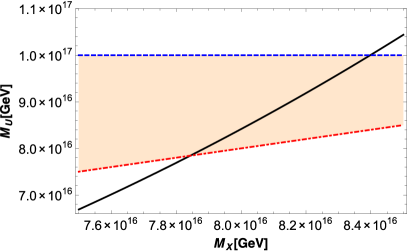
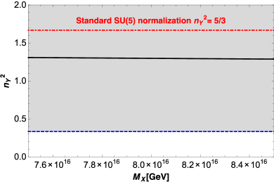
Figure 1: (Left) Allowed range for $\mathrm{SU(3)_{c}\otimes SU(3)_{L}\otimes U(1)_{X}}$ symmetry breaking scale $M_{X}$ for guaranteed unification. The solid line represents $M_{U}$ as a function of $M_{X}$. The dashed and dot-dashed lines correspond to $M_{U}=10^{17}$ GeV and $M_{U}=M_{X}$ respectively. (Right) The hypercharge normalization factor $n_{Y}^{2}$ as a function of the 331 symmetry breaking scale $M_{X}$. The shaded region represents the allowed region $n_{Y}^{2}\geq\frac{1}{3}$ with the dashed line corresponding to the lower limit $n_{Y}^{2}=\frac{1}{3}$. The solid line gives $n_{Y}^{2}$ as a function of $M_{X}$ and the red dot-dashed line shows the standard $SU(5)$ normalization $n_{Y}^{2}=\frac{5}{3}$.

In Fig. 1 (left) we plot the allowed range for $M_{X}$. The intersection of the line corresponding to $M_{U}$ evaluated as a function of $M_{X}$ in Eq. (24) with the lines for $M_{U}=M_{X}$ and $M_{U}=10^{17}$ GeV gives the lower and upper bound on $M_{X}$ respectively such that there is a guaranteed unification. In this scenario, the scale $M_{X}$ of $\mathrm{SU(3)_{c}\otimes SU(3)_{L}\otimes U(1)_{X}}$ breaking is therefore always high and very close to the unification scale $M_{U}$.

Next, in Fig. 1 (right) we plot the hypercharge normalization factor $n_{Y}^{2}$ as a function of $\mathrm{SU(3)_{c}\otimes SU(3)_{L}\otimes U(1)_{X}}$ symmetry breaking scale $M_{X}$. The dashed horizontal line represents the lower limit $n_{Y}^{2}=\frac{1}{3}$ of the allowed value for $n_{Y}^{2}$. As can be seen from the figure, for the allowed $M_{X}$ range from the condition $M_{X}\leq M_{U}\leq 10^{17}$ GeV the hypercharge normalization $n_{Y}^{2}$ is almost constant $\approx 1.3$ and well above the allowed lower limit.

Finally, in Fig. 2 we give an example of gauge coupling running with respect to the 331 symmetry breaking scale $M_{X}=7.9\times 10^{16}$ GeV. It demonstrates that successful gauge unification at the scale $M_{U}=8.05\times 10^{16}$ GeV with $n_{Y}^{2}=1.3$ can be achieved, albeit this requires a very high scale of $\mathrm{SU(3)_{c}\otimes SU(3)_{L}\otimes U(1)_{X}}$ breaking very near to the unification scale.

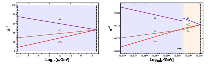
Figure 2: Gauge coupling running in the SVS Model with 331 symmetry breaking scale $M_{X}=7.9\times 10^{16}$ GeV, demonstrating successful gauge unification at the scale $M_{U}=8.05\times 10^{16}$ GeV with $n_{Y}^{2}=1.3$ . The right plot shows the magnified view of gauge coupling running around $M_{X}$.

IV.2 The SVS Model with fermionic octets

In this model, in addition to the field content of model I, we include three generations of fermion octets $\Omega$ with the assignments under the $\mathrm{SU(3)_{c}\otimes SU(3)_{L}\otimes U(1)_{X}}$ group given by

$${}\Omega\equiv[1,8^{\ast},0].$$ (26)

The Higgs sector involves the same three $\mathrm{SU(3)_{L}}$ triplets as before. Although this model has the same content as the one considered in Ref. Boucenna et al. (2015), here we take a completely different approach to unification. Indeed, we do not consider the usual SU(5) normalization for the hypercharge and the octet mass scale is the same as the 331 symmetry breaking scale. In this model, the neutrinos are massless at tree level, however at one-loop level the exchange of gauge bosons give rise to dimension-nine operator which generates neutrino masses after 331 symmetry breaking Boucenna et al. (2015). For the SM the one-loop beta-coefficients remain the same as Model I, while in the $\mathrm{SU(3)_{c}\otimes SU(3)_{L}\otimes U(1)_{X}}$ phase they are given by $b_{3L}=-1/2$, $b^{\text{UN}}_{X}=26/3$, $b^{X}_{3C}=-5$.

In Fig. 3 (left) we plot the allowed range for $M_{X}$ for which unification is guaranteed at a scale $M_{X}\leq M_{U}\leq 10^{17}$GeV. Interestingly, in this model we find that for a $\mathrm{SU(3)_{c}\otimes SU(3)_{L}\otimes U(1)_{X}}$ symmetry breaking scale $M_{X}$ as low as TeV it is possible to achieve unification. Note that in contrast to Ref. Boucenna et al. (2015), here we do not assume another intermediate scale corresponding to the fermion octet mass scale in addition to $M_{X}$. Formally, unification can thus be achieved for any scale $M_{X}$ between $M_{Z}$ and $M_{U}$, however, $M_{U}\lesssim 10^{15.5}$ GeV is disfavored by the current experimental limits on the lifetime of the proton decay Olive et al. (2014). This consequently puts a lower limit of the order of $M_{X}\gtrsim 10^{5}$ GeV on the $\mathrm{SU(3)_{c}\otimes SU(3)_{L}\otimes U(1)_{X}}$ breaking scale, although we should emphasize that we here do not specify the GUT group and thus cannot predict the proton decay rate accurately.

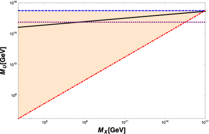
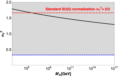
Figure 3: Same as Fig. 1, but for the $\mathrm{SU(3)_{c}\otimes SU(3)_{L}\otimes U(1)_{X}}$ SVS model with three additional fermionic octets. The purple dotted line corresponds to the lower limit of $M_{U}$ allowed by the current experimental limits on the lifetime of the proton decay.

In Fig. 3 (right) we plot the hypercharge normalization factor $n_{Y}^{2}$ as a function of $\mathrm{SU(3)_{c}\otimes SU(3)_{L}\otimes U(1)_{X}}$ symmetry breaking scale $M_{X}$. In this case as well, for the allowed $M_{X}$ range from the condition $M_{X}\leq M_{U}\leq 10^{17}$ GeV the hypercharge normalization $n_{Y}^{2}$ is well above its allowed lower limit.

In Fig. 4 we show an example gauge coupling running with $\mathrm{SU(3)_{c}\otimes SU(3)_{L}\otimes U(1)_{X}}$ symmetry breaking scale $M_{X}=3000$ GeV, demonstrating successful gauge coupling unification at a scale $M_{U}=10^{14.9}$ GeV with $n_{Y}^{2}=1.8$. Thus, from the perspective of a low $\mathrm{SU(3)_{c}\otimes SU(3)_{L}\otimes U(1)_{X}}$ symmetry breaking scale within the reach of accelerator experiments like the LHC $\sim{\mathcal{O}}$(TeV)) this model is the most interesting candidate leading to a successful gauge coupling unification. In addition to the new gauge bosons, the model can harbor a plethora of new states associated to the new exotic fermions as well as extra Higgs bosons.

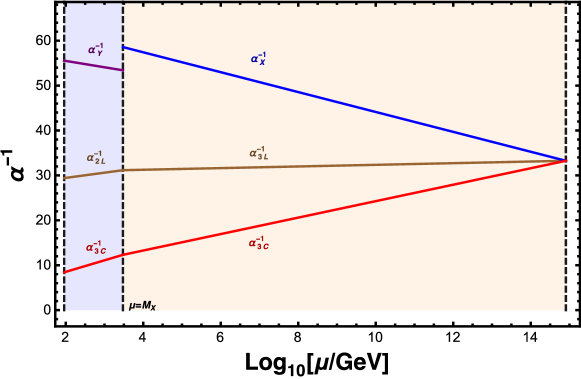
Figure 4: Gauge coupling running in the SVS Model adding three generations of leptonic octets with $\mathrm{SU(3)_{c}\otimes SU(3)_{L}\otimes U(1)_{X}}$ symmetry breaking scale at $M_{X}=3000$ GeV, demonstrating successful gauge unification at the scale $M_{U}=10^{14.9}$ GeV with $n_{Y}^{2}=1.8$.

V SU(6) Grand Unification

We consider the possibility of grand unification of the $\mathrm{SU(3)_{c}\otimes SU(3)_{L}\otimes U(1)_{X}}$ model in an SU(6) gauge unification group. Two possibilities arise. Unlike other conventional grand unified theories, in SU(6) one can have different components of the 331 subgroup with different multiplicity. Such a scenario may emerge from the flux breaking of the unified group in an E(6) F-theory GUT. This provides new ways of achieving gauge coupling unification in 331 models. Alternatively, a sequential variant of $\mathrm{SU(3)_{c}\otimes SU(3)_{L}\otimes U(1)_{X}}$ model can have a minimal SU(6) grand unification, which in turn can be a natural E(6) subgroup. This minimal SU(6) embedding does not require any bulk exotics to account for the chiral families and allows for a TeV scale $\mathrm{SU(3)_{c}\otimes SU(3)_{L}\otimes U(1)_{X}}$ model.

We now demonstrate how the $\mathrm{SU(3)_{c}\otimes SU(3)_{L}\otimes U(1)_{X}}$ model fermions can be embedded in an SU(6) grand unified gauge group. Our main consideration is to explore whether the combinations of the SU(6) gauge group representations form an anomaly free set, which can contain all the required fermions. In the subsequent subsections we discuss how different multiplicities of the SVS version of the $\mathrm{SU(3)_{c}\otimes SU(3)_{L}\otimes U(1)_{X}}$ model can be explained when this SU(6) grand unified model is embedded in an E(6) F-theory and how the sequential $\mathrm{SU(3)_{c}\otimes SU(3)_{L}\otimes U(1)_{X}}$ model can be embedded in a minimal anomaly free combination of representations of SU(6) as an E(6) subgroup. For the minimal SVS version of the $\mathrm{SU(3)_{c}\otimes SU(3)_{L}\otimes U(1)_{X}}$ model, gauge coupling unification can be obtained by including both the matter multiplets in the 27-dimensional fundamental representations of E(6) as well as the bulk exotics from the 78-dimensional adjoint representations of E(6). In particular the octet of $\mathrm{SU(3)_{L}}$ coming from the bulk plays a crucial role in allowing the unification of the gauge couplings with a low 331 symmetry breaking scale. On the other hand, the embedding of sequential 331 model in SU(6) does not require any bulk exotics to account for the chiral multiplets and imply, by adding three generations of $\mathrm{U(1)_{X}}$ neutral fermionic octets, one can obtain SU(6) unification with a TeV scale $\mathrm{SU(3)_{c}\otimes SU(3)_{L}\otimes U(1)_{X}}$ breaking scale.

We shall first write down some of the product decompositions of the group SU(6):

$${}6\times 6 = 15_{a}+21_{s},$$

$$6\times\bar{6} = 1+35,$$

$$6\times 15 = 20+70,$$

$$6\times 21 = 56+70.$$ (27)

The SU(6) has $\mathrm{SU(3)_{c}\otimes SU(3)_{L}\otimes U(1)_{X}}$ as a maximal subgroup with the same rank. For convenience we write down some of the representations of SU(6) under this maximal subgroup $\mathrm{SU(3)_{c}\otimes SU(3)_{L}\otimes U(1)_{X}}$:

$${}6 = [3,~{}1,~{}-1/3]~{}+~{}[1,~{}3,~{}1/3],$$

$$15 = [\bar{3},~{}1,~{}-2/3]~{}+~{}[1,~{}\bar{3},~{}2/3]~{}+~{}[3,~{}3,~{}0],$$

$$20 = [1,~{}1,~{}-1]~{}+~{}[1,~{}1,~{}1]~{}+~{}[3,~{}\bar{3},~{}1/3]~{}+~{}[\bar{3},~{}3,~{}-1/3],$$

$$21 = [3,~{}3,~{}0]~{}+~{}[6,~{}1,~{}-2/3]~{}+~{}[1,~{}6,~{}2/3],$$

$$35 = [1,~{}1,~{}0]~{}+~{}[8,~{}1,~{}0]~{}+~{}[1,~{}8,~{}0]~{}+~{}[3,~{}\bar{3},~{}-2/3]~{}+~{}[\bar{3},~{}3,~{}2/3],$$

$$56 = [10,~{}1,~{}-1]~{}+~{}[1,~{}10,~{}1]~{}+~{}[6,~{}3,~{}-1/3]~{}+~{}[3,~{}6,~{}1/3],$$

$$70 = [6,3,-1/3]+[3,6,-1/3]+[3,\bar{3},1/3]+[\bar{3},3,-1/3]+[8,1,-1]+[1,8,1].$$ (28)

The anomaly for the various representations of the group SU(6) are

$${}{\cal A}[6]=1,~{}{\cal A}[15]=2,~{}{\cal A}[20]=0,~{}{\cal A}[21]=10,~{}{\cal A}[35]=0,~{}{\cal A}[56]=54,~{}{\cal A}[70]=27.$$ (29)

We now turn to two concrete model constructions.

V.1 SU(6) Grand Unification of the SVS Model

It can be easily verified that all fermions of the $\mathrm{SU(3)_{c}\otimes SU(3)_{L}\otimes U(1)_{X}}$ model proposed by SVS (discussed in section II) can be included in the anomaly free combination of representations under SU(6):

$$\bar{6}~{}+~{}\bar{6}~{}+~{}15~{}+~{}20.$$

There will be some extra fermions and the multiplicity of the different representations are now different. It is to be noted that these states can be naturally embedded in an E(6) theory. We start with the maximal $\mathrm{SU(2)\times SU(6)}$ subgroup of E(6), and write down the decomposition:

$${}27 = [2,~{}\bar{6}]~{}+~{}[1,~{}15]$$

$$78 = [1,~{}35]~{}+~{}[2,~{}20]~{}+~{}[3,~{}1]$$

Thus the $\mathrm{SU(3)_{c}\otimes SU(3)_{L}\otimes U(1)_{X}}$ anomaly free representations of the SVS model can all be embedded in a combination of anomaly free representations of SU(6), which in turn can be embedded in the fundamental and adjoint representations of the group E(6). The next question is how to match the multiplicity of the different representations of the SVS 331 model, which is nontrivial. At this stage we resort to the symmetry breaking at the GUT scale induced by flux breaking through the Hosotani mechanism Hosotani (1989). Assigning particular geometry to the flux breaking, we identify the different states with the different algebraic varieties, and then the intersection numbers would give us the multiplicities of the different representations. A detailed study of such E(6) F-theory GUTs Beasley et al. (2009); King et al. (2010); Callaghan et al. (2012, 2013) is beyond the scope of this article and we shall rather take a phenomenological approach to the problem. We consider the required representations to match the low energy phenomenological requirements. The first step is to keep the known fermions light and also to have $\mathrm{SU(3)_{c}\otimes SU(3)_{L}\otimes U(1)_{X}}$ symmetry breaking scale as low as TeV, while at the same time requiring for gauge coupling unification.

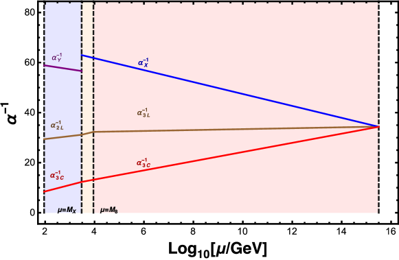
Figure 5: Gauge coupling running in the SVS Model with three generations of leptonic octets with 331 symmetry breaking scale $M_{X}=3000$ GeV and octet mass scale $M_{8}=9000$ GeV, demonstrating successful gauge unification at the scale $M_{U}=10^{15.5}$ GeV with $n_{Y}=\sqrt{5/3}$ and $n_{X}=2/\sqrt{3}$.

Considering the $\bar{6}$ representation of SU(6), which contains the down antiquarks $d^{c}_{L}$ with hypercharge $Y=1/3$, isospin lepton doublet containing $e_{L}$ and $\nu_{L}$ with $Y=-1/2$, and $N_{L}$ with $Y=0$; we can get the normalization for the hypercharge from $Tr(Y^{2})=5/6n^{-2}_{Y}$ in the notation of Eq. (19). The $\mathrm{U(1)_{Y}}$ normalization defined in Eq. (19) is given by $n_{Y}=\sqrt{5/3}$ and using Eq. (20) we obtain the $\mathrm{U(1)_{X}}$ normalization given by $n_{X}=2/\sqrt{3}$, which is below the normalizations required for a guaranteed unification in Fig. 1 and Fig. 3. However, it is still possible to obtain gauge coupling unification following the prescription in Ref. Boucenna et al. (2015), where the octet scale is decoupled from the $\mathrm{SU(3)_{c}\otimes SU(3)_{L}\otimes U(1)_{X}}$ symmetry breaking scale and is assumed to lie between the $\mathrm{SU(3)_{c}\otimes SU(3)_{L}\otimes U(1)_{X}}$ symmetry breaking scale and unification scale. Here, the octets belong to 35 of SU(6), which belongs to the bulk exotics coming from the 78-dimensional adjoint representations of E(6).

Using Eq. (LABEL:4.3) the the one-loop beta-coefficients $b_{i}$ can be calculated for the different phases. For the phase between the electroweak symmetry breaking scale and the $\mathrm{SU(3)_{c}\otimes SU(3)_{L}\otimes U(1)_{X}}$ symmetry breaking scale ($M_{Z}$ to $M_{X}$) the one-loop beta-coefficients are given by $b_{2L}=-19/6$, $b_{Y}=41/10$, $b_{3C}=-7$. For the phase between the $\mathrm{SU(3)_{c}\otimes SU(3)_{L}\otimes U(1)_{X}}$ symmetry breaking scale and the octet mass scale ($M_{X}$ to $M_{8}$) the one-loop beta-coefficients are given by $b_{3L}=-13/2$, $b_{X}=13/2$, $b^{331}_{3C}=-5$. Finally, for the phase between the octet mass scale to the unification scale ($M_{8}$ to $M_{U}$) the one-loop beta-coefficients are given by $b^{8}_{3L}=2n-13/2$, where $n$ is the number of generations of the fermionic octets ($\Omega\equiv[1,8^{\ast},0]$), $b^{8}_{X}=13/2$, $b^{8}_{3C}=-5$.

In Fig. 5 we plot the gauge coupling running of SVS $\mathrm{SU(3)_{c}\otimes SU(3)_{L}\otimes U(1)_{X}}$ model with the field content given in Eqs. (II,4) and three generations of fermionic octets with $\mathrm{SU(3)_{c}\otimes SU(3)_{L}\otimes U(1)_{X}}$ symmetry breaking scale $M_{X}=3000$ GeV and octet mass scale $M_{8}=9000$ GeV, demonstrating successful gauge unification at the scale $M_{U}=10^{15.5}$ GeV with $n_{Y}=\sqrt{5/3}$ and $n_{X}=2/\sqrt{3}$. A relative modest variation of the octet mass scale from the $\mathrm{SU(3)_{c}\otimes SU(3)_{L}\otimes U(1)_{X}}$ scale, $M_{8}/M_{X}=3$, therefore lifts the scale of successful unification from the value $M_{U}=10^{14.9}$ GeV found in Fig. 4 and thus relaxes the tension with proton decay limits, cf. Section VI.

V.2 SU(6) Grand Unification of the sequential $\mathrm{SU(3)_{c}\otimes SU(3)_{L}\otimes U(1)_{X}}$ Model

It is easy to verify from Eq. (V) that each generation of the fermionic multiplets of the sequential 331 model written in Eq. (III) fits perfectly in the anomaly free combination of SU(6) representations: $\bar{6}~{}+~{}\bar{6^{\prime}}~{}+~{}15$, where $\bar{6}$ contains $d^{c}_{L}\equiv[3,1,-1/3]$ and $\psi_{L}\equiv[1,3^{\ast},-1/3]$; $\bar{6^{\prime}}$ contains $D^{c}_{L}\equiv[3,1,-1/3]$ and $\xi_{L}\equiv[1,3^{\ast},-1/3]$; and $15$ contains $u^{c}_{L}\equiv[3^{\ast},1,-2/3]$, $\chi_{L}\equiv[1,3^{\ast},2/3]$ and $Q_{L}\equiv[3,3,0]$. Now the fundamental $27$ of E(6) branches under the maximal $\mathrm{SU(2)\otimes SU(6)}$ subgroup as $27=[2,~{}\bar{6}]~{}+~{}[1,~{}15]$. Thus three $27$s of E(6) contain three sets of $\bar{6}~{}+~{}\bar{6^{\prime}}~{}+~{}15$ accommodating the three generations of the fermionic multiplets of the sequential 331 model. However the minimal content of the sequential 331 model does not have a low scale unification. However, by adding three generations of fermionic octets again leads to a successful gauge coupling unification.

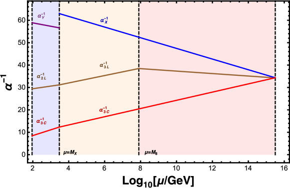
Figure 6: Gauge coupling running in the sequential 331 Model with three generations of fermionic octets with $\mathrm{SU(3)_{c}\otimes SU(3)_{L}\otimes U(1)_{X}}$ symmetry breaking scale $M_{X}=3000$ GeV and octet mass scale $M_{8}=8\times 10^{7}$ GeV, demonstrating successful gauge unification at the scale $M_{U}=10^{15.5}$ GeV with $n_{Y}=\sqrt{5/3}$ and $n_{X}=2/\sqrt{3}$.

For the phase between the electroweak symmetry breaking scale and the $\mathrm{SU(3)_{c}\otimes SU(3)_{L}\otimes U(1)_{X}}$ symmetry breaking scale ($M_{Z}$ to $M_{X}$) the one-loop beta-coefficients are given by $b_{2L}=-19/6$, $b_{Y}=41/10$, $b_{3C}=-7$. For the phase between the $\mathrm{SU(3)_{c}\otimes SU(3)_{L}\otimes U(1)_{X}}$ symmetry breaking scale and the octet mass scale ($M_{X}$ to $M_{8}$) the one-loop beta-coefficients are given by $b_{3L}=-9/2$, $b_{X}=13/2$, $b^{331}_{3C}=-5$. Finally, for the phase between the octet mass scale to the unification scale ($M_{8}$ to $M_{U}$) the one-loop beta-coefficients are given by $b^{8}_{3L}=2n-9/2$, where $n$ is the number of generations of the fermionic octets ($\Omega\equiv[1,8^{\ast},0]$), $b^{8}_{X}=13/2$, $b^{8}_{3C}=-5$.

In Fig. 6 we plot the gauge coupling running of the sequential $\mathrm{SU(3)_{c}\otimes SU(3)_{L}\otimes U(1)_{X}}$ model with the field content given in Eqs. (4,III) and three generations of fermionic octets with $\mathrm{SU(3)_{c}\otimes SU(3)_{L}\otimes U(1)_{X}}$ symmetry breaking scale $M_{X}=3000$ GeV and octet mass scale $M_{8}=8\times 10^{7}$ GeV, demonstrating successful gauge unification at the scale $M_{U}=10^{15.5}$ GeV with $n_{Y}=\sqrt{5/3}$ and $n_{X}=2/\sqrt{3}$. In this scenario, the octet mass scale has to be detached rather strongly from the $\mathrm{SU(3)_{c}\otimes SU(3)_{L}\otimes U(1)_{X}}$ scale in order to achieve successful unification.

VI $\sin^{2}\theta_{w}$ and proton decay in SU(6) grand unification

Using the RGEs and the relations among the coupling constants corresponding to different gauge groups one can express $\sin^{2}\theta_{w}(M_{Z})$ in terms of the different scales associated with the SU(6) grand unified theory. Noting that for SU(6) grand unification we have $n_{Y}=\sqrt{5/3}$ and $n_{X}=2/\sqrt{3}$, the relation between normalized couplings at the scales $M_{Z}$ and $M_{X}$ are given by

$${}\alpha_{2L}^{-1}(M_{Z}) = \alpha_{\rm{em}}^{-1}(M_{Z})-\frac{5}{3}{\alpha^{N}_{Y}}^{-1}(M_{Z}),$$ (30)

$${\alpha^{N}_{Y}}^{-1}(M_{X}) = \frac{1}{5}\alpha_{3L}^{-1}(M_{X})+\frac{4}{5}{\alpha^{N}_{X}}^{-1}(M_{X}).{}$$ (31)

Using Eq. (30) it is straightforward to obtain

$${}\sin^{2}\theta_{w}(M_{Z})\equiv\frac{\alpha_{\rm{em}}(M_{Z})}{\alpha_{2L}(M_{Z})}=\frac{3}{8}+\frac{5}{8}\alpha_{\rm{em}}(M_{Z})\left[\alpha_{2L}^{-1}(M_{Z})-{\alpha^{N}_{Y}}^{-1}(M_{Z})\right].$$ (32)

Finally, using Eqs. (14), (31) the above equation can be written in the form

$${}\sin^{2}\theta_{w}(M_{Z})= \frac{3}{8}+\frac{5}{8}\alpha_{\rm{em}}(M_{Z})\left[\frac{4}{5}\left\{\frac{b_{3L}}{2\pi}\ln\left(\frac{M_{8}}{M_{X}}\right)+\frac{b_{3L}^{8}}{2\pi}\ln\left(\frac{M_{U}}{M_{8}}\right)\right\}\right.$$ (33)

$$\left.+\frac{(b_{2L}-b_{Y})}{2\pi}\ln\left(\frac{M_{X}}{M_{Z}}\right)-\frac{4}{5}\frac{b_{X}}{2\pi}\ln\left(\frac{M_{U}}{M_{X}}\right)\right],$$

which can be readily used to obtain the prediction for $\sin^{2}\theta_{w}(M_{Z})$. For example, in the sequential 331 model taking $\mathrm{SU(3)_{c}\otimes SU(3)_{L}\otimes U(1)_{X}}$ symmetry breaking scale $M_{X}=3000$ GeV, octet mass scale $M_{8}=8\times 10^{7}$ GeV, and unification scale $M_{U}=10^{15.5}$ GeV we obtain $\sin^{2}\theta_{w}(M_{Z})\simeq 0.231$, which is consistent with the electroweak precision data Olive et al. (2014).

Turning to the prediction for proton decay, we note that being a non-supersymmetric scenario the gauge $d=6$ contributions for proton decay are most important here. An analysis of all $\mathrm{SU(3)_{c}\otimes SU(2)_{L}\otimes U(1)_{Y}}$ invariant operators Weinberg (1979, 1980); Wilczek and Zee (1979); Weldon and Zee (1980) that can induce proton decay in SU(6) is beyond the scope of this article and will be addressed in a separate communication. Here we will consider the decay mode $p\rightarrow e^{+}\pi^{0}$, which is constrained by experimental searches to have a life time $\tau^{\rm{expt}}_{p}\geq 1\times 10^{34}$ Olive et al. (2014). The relevant effective operators in the physical basis are given by Fileviez Perez (2004); Nath and Fileviez Perez (2007)

$${}\mathcal{O}(e^{c}_{\alpha},d_{\beta}) = c(e^{c}_{\alpha},d_{\beta})\epsilon_{ijk}\overline{u^{c}_{i}}_{L}\gamma^{\mu}u_{jL}\overline{e^{c}_{\alpha}}_{L}\gamma_{\mu}{d_{k\beta}}_{L},$$

$$\mathcal{O}(e_{\alpha},d^{c}_{\beta}) = c(e_{\alpha},d^{c}_{\beta})\epsilon_{ijk}\overline{u^{c}_{i}}_{L}\gamma^{\mu}u_{jL}\overline{d^{c}_{k\beta}}_{L}\gamma_{\mu}{e_{\alpha}}_{L};$$ (34)

where

$${}c(e^{c}_{\alpha},d_{\beta}) = k_{1}^{2}\left[V^{11}_{1}V^{\alpha\beta}_{2}+(V_{1}V_{UD})^{1\beta}(V_{2}V_{UD}^{\dagger})^{\alpha 1}\right],$$

$$c(e_{\alpha},d^{c}_{\beta}) = k_{1}^{2}V^{11}_{1}V^{\beta\alpha}_{3}+k^{2}_{2}(V_{4}V_{UD}^{\dagger})^{\beta 1}+(V_{1}V_{UD}V_{4}^{\dagger}V_{3})^{1\alpha};$$

$$\alpha = \beta\neq 2.$$ (35)

Here $i,j,k=1,2,3$ are the color indices and $\alpha,\beta=1,2$; $V_{1,2,3,4}$ and $V_{UD}$ are the mixing matrices $V_{1}=U^{\dagger}_{C}U$, $V_{2}=E^{\dagger}_{C}D$, $V_{3}=D^{\dagger}_{C}E$, $V_{UD}=U^{\dagger}D$; where $U,D,E$ are the unitary matrices diagonalizing the Yukawa couplings e,g. $U^{T}_{C}Y_{U}U=Y_{U}^{\rm{diag}}$. $k_{1}=g_{\rm{GUT}}/M_{(X,Y)}$ and $k_{2}=g_{\rm{GUT}}/M_{(X^{\prime},Y^{\prime})}$, where $M_{(X,Y)},M_{(X^{\prime},Y^{\prime})}\sim M_{\rm{GUT}}$ are the masses of the superheavy gauge bosons and $g_{\rm{GUT}}$ is the coupling constant at the GUT scale. The decay rate for $p\rightarrow e^{+}\pi^{0}$ mode is given by

$${}\Gamma(p\rightarrow e^{+}\pi^{0})=\frac{m_{p}}{16\pi f_{\pi}^{2}}A_{L}^{2}|\alpha_{H}|^{2}(1+D+F)^{2}\left[|c(e,d^{c})|^{2}+|c(e^{c},d)|^{2}\right],$$ (36)

where $m_{p}=938.3$ MeV is the proton mass, $f_{\pi}=139$ MeV is the pion decay constant, $A_{L}$ is the long distance renormalization factor; $D,F$ and $\alpha_{H}$ are parameters of the chiral Lagrangian. For a rough estimate, taking $\alpha_{H}(1+D+F)\sim 0.012~{}{\rm{GeV}}^{3}$ Aoki et al. (2007, 2008); $A_{R}=A_{L}A^{\rm{SD}}_{R}\sim 3$, where $A^{\rm{SD}}_{R}$ is the short distance renormalization factor; the parameter depending on the mixing matrices $F_{q}(V)\sim 5$, we obtain

$${}\Gamma^{-1}(p\rightarrow e^{+}\pi^{0})\sim 10^{36}\text{ yrs}\left(\frac{\alpha^{-1}_{\text{GUT}}}{35}\right)^{2}\left(\frac{M_{U}}{10^{16}\text{ GeV}}\right)^{4}.$$ (37)

Now noting that $M_{U}=10^{15.5}$ GeV and $\alpha^{-1}_{\rm{GUT}}\sim 35$ in the SVS and sequential 331 models, the lifetime of the proton decay mode $p\rightarrow e^{+}\pi^{0}$ comes out to be $\sim 10^{34}$ yrs, which is consistent with the current experimental limit Olive et al. (2014).

VII Discussion and outlook

In this paper we have considered the possibility of conventional non-supersymmetric grand unification of extended electroweak models based upon the $\mathrm{SU(3)_{c}\otimes SU(3)_{L}\otimes U(1)_{X}}$ gauge framework within an SU(6) gauge unification group. In contrast to other conventional grand unified theories, in SU(6) one can have different components of the $\mathrm{SU(3)_{c}\otimes SU(3)_{L}\otimes U(1)_{X}}$ subgroup with different multiplicity. Such scenarios may emerge from the flux breaking of the unified group in an E(6) F-theory GUT framework. While it allows for successful unification, the required 331 scale is typically very close to unification.

However, the sequential addition of a leptonic octet provides a way of achieving gauge coupling unification at 331 scales accessible at collider experiments. Alternatively, we have also considered a sequential variant of the $\mathrm{SU(3)_{c}\otimes SU(3)_{L}\otimes U(1)_{X}}$ model that can have a minimal SU(6) grand unification, which in turn can be a natural E(6) subgroup. Such minimal SU(6) embedding does not require any bulk exotics in order to account for the chiral families and allows for a TeV scale $\mathrm{SU(3)_{c}\otimes SU(3)_{L}\otimes U(1)_{X}}$ model as well as seesaw-induced neutrino masses.

In both cases the gauge coupling unification is associated to the presence of sequential a leptonic octet at some intermediate scale between the 331 scale, which lies in the TeV range, and the unification scale. It is important to stress that the presence of the octet plays a key role in the mechanism of neutrino mass generation. In other words, the same physics that drives unification is responsible for the radiative origin of neutrino masses Boucenna et al. (2015).

References

- Singer et al. (1980) M. Singer, J. Valle, and J. Schechter, Phys.Rev. D22, 738 (1980).
- Valle and Singer (1983) J. W. F. Valle and M. Singer, Phys. Rev. D28, 540 (1983).
- Boucenna et al. (2014) S. M. Boucenna, S. Morisi, and J. W. F. Valle, Phys. Rev. D90, 013005 (2014), eprint 1405.2332.
- Boucenna et al. (2015) S. M. Boucenna, R. M. Fonseca, F. Gonzalez-Canales, and J. W. F. Valle, Phys. Rev. D91, 031702 (2015), eprint 1411.0566.
- Addazi et al. (2016) A. Addazi, J. W. F. Valle, and C. A. Vaquera-Araujo, Phys. Lett. B759, 471 (2016), eprint 1604.02117.
- Gursey et al. (1976) F. Gursey, P. Ramond, and P. Sikivie, Phys. Lett. B60, 177 (1976).
- Beasley et al. (2009) C. Beasley, J. J. Heckman, and C. Vafa, Journal of High Energy Physics 2009, 059 (2009), URL http://stacks.iop.org/1126-6708/2009/i=01/a=059.
- King et al. (2010) S. F. King, G. K. Leontaris, and G. G. Ross, Nucl. Phys. B838, 119 (2010), eprint 1005.1025.
- Callaghan et al. (2012) J. C. Callaghan, S. F. King, G. K. Leontaris, and G. G. Ross, JHEP 04, 094 (2012), eprint 1109.1399.
- Callaghan et al. (2013) J. C. Callaghan, S. F. King, and G. K. Leontaris, JHEP 12, 037 (2013), eprint 1307.4593.
- Georgi and Glashow (1974) H. Georgi and S. Glashow, Phys.Rev.Lett. 32, 438 (1974).
- Sanchez et al. (2001) L. A. Sanchez, W. A. Ponce, and R. Martinez, Phys. Rev. D64, 075013 (2001), eprint hep-ph/0103244.
- Georgi et al. (1974) H. Georgi, H. R. Quinn, and S. Weinberg, Phys. Rev. Lett. 33, 451 (1974).
- Olive et al. (2014) K. Olive et al. (Particle Data Group), Chin.Phys. C38, 090001 (2014).
- Hosotani (1989) Y. Hosotani, Annals of Physics 190, 233 (1989), ISSN 0003-4916, URL http://www.sciencedirect.com/science/article/pii/0003491689900158.
- Weinberg (1979) S. Weinberg, Phys. Rev. Lett. 43, 1566 (1979).
- Weinberg (1980) S. Weinberg, Phys. Rev. D22, 1694 (1980).
- Wilczek and Zee (1979) F. Wilczek and A. Zee, Phys. Rev. Lett. 43, 1571 (1979).
- Weldon and Zee (1980) H. A. Weldon and A. Zee, Nucl. Phys. B173, 269 (1980).
- Fileviez Perez (2004) P. Fileviez Perez, Phys. Lett. B595, 476 (2004), eprint hep-ph/0403286.
- Nath and Fileviez Perez (2007) P. Nath and P. Fileviez Perez, Phys. Rept. 441, 191 (2007), eprint hep-ph/0601023.
- Aoki et al. (2007) Y. Aoki, C. Dawson, J. Noaki, and A. Soni, Phys. Rev. D75, 014507 (2007), eprint hep-lat/0607002.
- Aoki et al. (2008) Y. Aoki, P. Boyle, P. Cooney, L. Del Debbio, R. Kenway, C. M. Maynard, A. Soni, and R. Tweedie (RBC-UKQCD), Phys. Rev. D78, 054505 (2008), eprint 0806.1031.