Phase diagram and spin correlations of the Kitaev-Heisenberg model:
Importance of quantum effects

Abstract

We explore the phase diagram of the Kitaev-Heisenberg model with nearest neighbor interactions on the honeycomb lattice using the exact diagonalization of finite systems combined with the cluster mean field approximation, and supplemented by the insights from the linear spin-wave and second–order perturbation theories. This study confirms that by varying the balance between the Heisenberg and Kitaev term, frustrated exchange interactions stabilize in this model four phases with magnetic long range order: Néel phase, ferromagnetic phase, and two other phases with coexisting antiferromagnetic and ferromagnetic bonds, zigzag and stripy phases. They are separated by two disordered quantum spin-liquid phases, and the one with ferromagnetic Kitaev interactions has a substantially broader range of stability as the neighboring competing ordered phases, ferromagnetic and stripy, have very weak quantum fluctuations. Focusing on the quantum spin-liquid phases, we study spatial spin correlations and dynamic spin structure factor of the model by the exact diagonalization technique, and discuss the evolution of gapped low-energy spin response across the quantum phase transitions between the disordered spin liquid and magnetic phases with long range order.

I Introduction

Frustration in magnetic systems occurs by competing exchange interactions and leads frequently to disordered spin-liquid states Nor09 ; Bal10 ; Lucile . Recent progress in understanding transition metal oxides with orbital degrees of freedom demonstrated many unusual properties of systems with active $t_{2g}$ degrees of freedom — they are characterized by anisotropic hopping Kha00 ; Har03 ; Dag08 ; Nic11 ; Wro10 which generates Ising-like orbital interactions Jac04 ; Kha05 ; Jac07 ; Jac08 ; Kru09 ; Che09 ; Ryn10 ; Tro12 ; Che13 , similar to the orbital superexchange in $e_{g}$ systems Dag04 ; Rei05 . Particularly challenging are $4d$ and $5d$ transition metal oxides, where the interplay between strong electron correlations and spin-orbit interaction leads to several novel phases Wit14 ; Brz15 . In iridates the spin-orbit interaction is so strong that spins and orbital operators combine to new $S=1/2$ pseudospins at each site Jac09 , and interactions between these pseudospins decide about the magnetic order in the ground state.

The $A_{2}$IrO₃ ($A$=Na, Li) family of honeycomb iridates has attracted a lot of attention as these compounds have $t_{2g}$ orbital degree of freedom and lie close to the exactly solvable $S=1/2$ Kitaev model Kit06 . This model has a number of remarkable features, including the absence of any symmetry breaking in its quantum Kitaev spin-liquid (KSL) ground state, with gapless Majorana fermions Kit06 and extremely short-ranged spin correlations Bas07 . We emphasize that below we call a KSL also disordered spin-liquid states which arise near the Kitaev points in presence of perturbing Heisenberg interactions $\propto J$.

By analyzing possible couplings between the Kramers doublets it was proposed that the microscopic model adequate to describe the honeycomb iridates includes Kitaev interactions accompanied by Heisenberg exchange in form of the Kitaev-Heisenberg (KH) model Jac09 ; Cha10 . Soon after the experimental evidence was presented that several features of the observed zigzag order are indeed captured by the KH model Sin10 ; Liu11 ; Sin12 ; Cho12 ; Ye12 ; Comin ; Gre13 ; Tro13 ; Cha13 . Its parameters for $A_{2}$IrO₃ compounds are still under debate at present Kat14 ; Val16 . One finds also a rather unique crossover from the quasiparticle states to a non-Fermi liquid behavior by varying the frustrated interactions Tro14 . Unfortunately, however, it was recently realized that this model does not explain the observed direction of magnetic moments in Na₂IrO₃ and its extension is indeed necessary to describe the magnetic order in real materials Chu15 ; Cha15 . For example, bond-anisotropic interactions associated with the trigonal distortions have to play a role to explain the differences between Na₂IrO₃ and Li₂IrO₃ Rau15 , the two compounds with quite different behavior reminiscent of the unsolved problem of NaNiO₂ and LiNiO₂ in spin-orbital physics Rei05 . On the other hand, the KH model might be applicable in another honeycomb magnet $\alpha$-RuCl₃, see e.g. a recent study of its spin excitation spectrum Ban16 .

Understanding the consequences of frustrated Heisenberg interactions on the honeycomb lattice is very challenging and has stimulated several studies Alb11 ; Cab11 ; Son16 . The KH model itself is highly nontrivial and poses an even more interesting problem in the theory Cha10 ; Cha13 ; Rau14 ; Oit15 : Kitaev term alone has intrinsic frustration due to directional Ising-like interactions between the spin components selected by the bond direction Kit06 . In addition, these interactions are disturbed by nearest neighbor Heisenberg exchange which triggers long-range order (LRO) sufficiently far from the Kitaev points Cha10 ; Cha13 ; Rau14 ; Oit15 . In general, ferromagnetic (FM) and antiferromagnetic (AF) interactions coexist and the phase diagram of the KH model is quite rich as shown in several previous studies Cha10 ; Cha13 ; Rau14 ; Oit15 ; Tre11 ; Ire14 . Finally, the KH model has also a very interesting phase diagram on the triangular lattice Li15 ; Bec15 ; Jac15 ; Rou16 . These studies motivate better understanding of quantum effects in the KH model on the honeycomb lattice in the full range of its competing interactions.

The first purpose of this paper is to revisit the phase diagram of the KH model and to investigate it further by combining exact diagonalization (ED) result Cha13 with the self-consistent cluster mean field theory (CMFT), supplemented by the insights from the linear spin-wave (LSW) theory and the second–order perturbation theory (SOPT). The main advantage of CMFT is that it goes beyond a single site mean field classical theory and gives not only the symmetry-broken states with LRO, but also includes partly quantum fluctuations, namely the ones within the considered clusters Alb11 ; Brz12 . In this way the treatment is more balanced and may allow for disordered states in cases when frustration of interactions dominates. We present below a complete CMFT treatment of the phase diagram which includes also the Kitaev term in MF part of the Hamiltonian and covers the entire parameter space (in contrast to the earlier prototype version of CMFT calculation on a single hexagon for the KH model Got15 ). Note that the CMFT complements the ED which is unable to get symmetry breaking for a finite system, but nevertheless can be employed to investigate the phase transitions in the present KH model by evaluating the second derivative of the ground state energy to identify phase transitions by its characteristic maxima Cha10 ; Cha13 . ED result can be also used to recognize the type of magnetic order by transforming to reciprocal space and computing spin-structure factor. The second purpose is to investigate further the difference between quantum KSL regions around both Kitaev points mentioned in Ref. Cha13 and LRO/KSL boundaries.

The paper is organized as follows: In Sec. II we introduce the KH model and define its parameters. In Sec. III we present three methods of choice: (i) the exact diagonalization in Sec. III.1, (ii) the self-consistent CMFT in Sec. III.2, and (iii) linear spin wave theory in Sec. III.4. An efficient method of solving the self-consistence problem obtained within the CMFT is introduced in Sec. III.3. The numerical results are presented and discussed in Sec. IV: (i) the phase transitions and the phase diagram are introduced in Sec. IV.1, and (ii) the phase boundaries, the values of the ground state energies and the magnetic moments obtained by different methods are presented and discussed in Secs. IV.2 and IV.3, and (iii) we discuss the compatibility of the Kitaev interaction with different spin ordered states in Sec. IV.3. Spin correlations obtained for various phases are presented in Sec. V. The dynamical spin susceptibility and spin structure factor are presented for different phases in Sec. VI. Finally, in Sec. VII we present the main conclusions and short summary. The paper is supplemented with Appendix where we explain the advantages of the linearization procedure implemented on the CMFT on the example of a single hexagon.

II Kitaev-Heisenberg Model

We start from the KH Hamiltonian with nearest neighbor interactions on the honeycomb lattice in a form,

$${\cal H} \equiv K\sum_{\langle ij\rangle\parallel\gamma}S_{i}^{\gamma}S_{j}^{\gamma}+J\sum_{\langle ij\rangle}\boldsymbol{S}_{i}\cdot\boldsymbol{S}_{j},$$ (1)

where $\gamma=x$,$y$,$z$ labels the bond direction. The Kitaev term $\propto K$ favors local bond correlations of the spin component interacting on the particular bond. The superexchange $J$ is of Heisenberg form and alone would generate a LRO state, antiferromagnetic or ferromagnetic, depending on whether $J>0$ or $J<0$. We fix the overall energy scale, $J^{2}+K^{2}=1$, and choose angular parametrization

$$K = \sin\varphi,$$ (2)

$$J = \cos\varphi,$$ (3)

varying $\varphi$ within the interval $\varphi\in[0,2\pi]$. This parametrization exhausts all the possibilities for nearest neighbor interactions in the KH model.

While zigzag AF order was observed in Na₂IrO₃ Sin12 ; Cho12 ; Ye12 ; Comin ; Gre13 , its microscopic explanation has been under debate for a long time. The ab initio studies Foy13 ; Kat15 give motivation to investigate a broad regime of parameters $K$ (2) and $J$ (3). Further motivation comes from the honeycomb magnet $\alpha$-RuCl₃ Ban16 . Note that we do not intend to identify the parameter sets representative for each individual experimental system, but shall concentrate instead on the phase diagram of the model Eq. (1) with nearest neighbor interactions only.

III Calculation methods

III.1 Exact diagonalization

We perform Lanczos diagonalization for $N=24$-site cluster with periodic boundary conditions (PBC). This cluster respects all the symmetries of the model, including hidden ones. Among the accessible clusters it is expected to have the minimal finite-size effects.

III.2 Cluster mean field theory

A method which combines ED with an explicit breaking of Hamiltonian’s symmetries is the so-called self-consistent CMFT. It has been applied to several models with frustrated interactions, including Kugel-Khomskii model Brz12 . The method was also extensively used by Albuquerque et al. Alb11 as one of the means to establish the full phase diagram of Heisenberg-$J_{2}$-$J_{3}$ model on the honeycomb lattice.

Within CMFT the internal bonds of the cluster [connecting the circles in Fig. 1(a)] are treated exactly. The corresponding part $H_{\rm IN}$ of the Hamiltonian is the nearest neighbor KH Hamiltonian, Eq. (1). The external bonds that connect the boundary sites ($\bullet$) with the corresponding boundary sites of periodic copies of the cluster ($\Box$) are described by the MF part of the Hamiltonian,

$$H_{\rm MF} \equiv K\sum_{[ij]\parallel z}\langle S_{i}^{z}\rangle S_{j}^{z}+J\sum_{[ij]}\langle S_{i}^{z}\rangle S^{z}_{j},$$ (4)

where $[ij]$ marks the external bonds. Since the ordered moments in KH model align always along one of the cubic axes $x$, $y$, $z$ (see e.g. Ref. Cha10 ) we have put

$$\langle\vec{S}_{i}\rangle\cdot\vec{S}_{j}\equiv\langle S^{z}_{i}\rangle S^{z}_{j}$$ (5)

in $H_{\rm MF}$ to simplify the calculations.

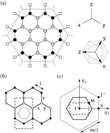
Figure 1: (a) 24-site cluster and the introduction of the mean fields. Gray (black) circles indicate internal (boundary) sites. In CMFT the internal bonds of the cluster are treated exactly while the external bonds crossing the cluster boundary (dashed) are treated on the MF level. The sites marked by $\Box$ generate an effective magnetic fields on the boundary sites $\bullet$. Labels $x$, $y$ and $z$ stand for three inequivalent bond directions determining the active products $S^{\gamma}_{i}S^{\gamma}_{j}$ in Kitaev part of the Hamiltonian (1), e.g. bonds of $x$ direction contribute with the $S^{x}_{i}S^{x}_{j}$ product to the Hamiltonian. The pseudospin axes used here are parallel to the cubic axes indicated in the top view of a single octahedron. (b) Unit cells: for honeycomb lattice (coinciding with single hexagon of that lattice), for triangular lattice (inner dotted hexagon) and zigzag magnetic unit cell (dashed rectangle). Black and white circles indicate one of three equivalent zigzag patterns. (c) Corresponding Brillouin zones and special $\boldsymbol{q}$ points for the lattice constant $a=1$.

The averages $\langle S_{i}^{z}\rangle$ generate effective magnetic fields acting on the boundary sites of the cluster. The total Hamiltonian

$${\cal H} \equiv H_{\rm IN}+H_{\rm MF},$$ (6)

is diagonalized in a self-consistent manner, taking slightly different approach than the one presented in Ref. Alb11 : instead of starting with random wave function our algorithm begins with expectation values $\langle S_{i}^{z}\rangle_{\mathrm{ini}}$ on each boundary site $i$ of the cluster. These can represent a certain pattern (zigzag, stripy, Néel, FM) or be set randomly to have a “neutral” starting point. After diagonalizing the Hamiltonian (6) (again by the ED Lanczos method) the ground state of the system is obtained and we recalculate the expectation values $\langle S^{z}_{i}\rangle$ to be used in the second iteration. The procedure is repeated until self-consistency is reached.

III.3 Linearized cluster mean field theory

A single iteration of the self-consistent MF calculation may be viewed as a nonlinear mapping of the set of initial averages $\{\langle S_{i}^{z}\rangle_{\mathrm{in}}\}$ to the resulting averages $\{\langle S_{i}^{z}\rangle_{\mathrm{fin}}\}$. The self-consistent solution is then a stable stationary point of such a mapping. To find the leading instability, we may consider the case of small initial averages in the CMFT calculation and identify the pattern characterized by the fastest growth during the iterations. To this end we linearize the above mapping.

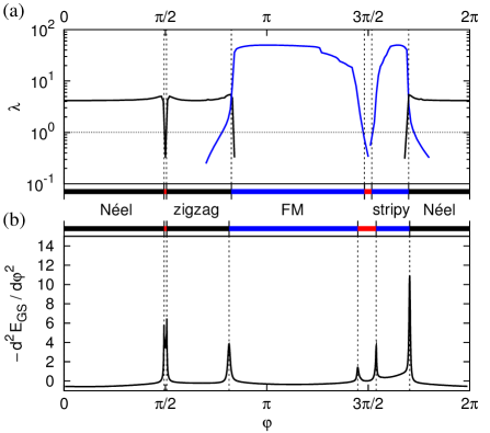
Figure 2: (a) The values of $\lambda$ obtained by the linearization of CMFT for an embedded cluster of $N=24$ sites with fixed magnetic order patterns: FM, AF, stripy, and zigzag. Leading $\lambda>1$ indicates the order that sets in. The disordered KSL phase is indicated by the red color. (b) Second derivative of the ground state energy, $-\mathrm{d}^{2}E_{0}(\varphi)/\mathrm{d}\varphi^{2}$, obtained by ED. Adopted from Ref. Cha13 .

In the lowest order the mapping corresponds to the multiplication of the vector of the averages $\{\langle S_{i}^{z}\rangle_{\mathrm{in}}\}$ by the matrix,

$$F_{ij}=\frac{\partial\langle S_{i}^{z}\rangle_{\mathrm{fin}}}{\partial\langle S_{j}^{z}\rangle_{\mathrm{in}}},$$ (7)

where $i$ and $j$ run through the cluster boundary sites. During iterations, the patterns corresponding to the individual eigenvectors of the matrix $F$ grow as $\lambda^{n}$, where $\lambda$ is a particular eigenvalue and $n$ is the number of iterations. The ordering pattern obtained by CMFT is then given by the eigenvector with largest $\lambda_{max}>1$. In the quantum KSL regimes, all the eigenvalues are less than $1$ and no magnetic order emerges. An example of linearized CMFT applied to a single hexagon with PBC can be found in the Appendix.

A modified version of this method, used to obtain Fig. 2(a), assumes a particular ordered pattern (Néel, zigzag, FM, or stripy phase) and uses a single spin average $\langle S^{z}\rangle_{\mathrm{in}}$ distributed along the boundary sites outside the cluster, with the signs consistent with this pattern. The resulting values, $\langle S^{z}_{i}\rangle_{\mathrm{fin}}$, are then averaged correspondingly. In this case the matrix $F$ is reduced to a single value $\lambda$ plotted in Fig. 2(a). We observe that the largest eigenvalue either drops below 1 when the disordered KSL state takes over, or interchanges with another eigenvalue corresponding to a different ordered phase.

III.4 Linear spin-wave theory

The LSW method is a basic tool to determine spin excitations and quantum corrections in systems with long-range order Wal63 . For systems with coexisting AF and FM bonds quantum corrections are smaller than for the Néel phase but are still substantial for $S=1/2$ spins Rac02 . For the KH model the LSW theory Cha10 ; Cha13 ; Cho12 has to be implemented separately for each of the four ordered ground states: Néel (N), zigzag (ZZ), FM, or stripy (ST). Then for a particular ground state the Hamiltonian is rewritten in terms of the Holstein-Primakoff bosons Cho12 ; Mak15 and only quadratic terms in bosonic operators are kept. The spectrum of such quadratic Hamiltonian is finally obtained using the successive Fourier and Bogoliubov transformations.

While the spin wave dispersion relations are usually of prime interest Cho12 ; Mak15 ; Cha10 ; Cha13 , there are also two other quantities which can easily be calculated using LSW and which will be important in the discussion that follows: (i) the value of the total ordered moment $\langle M\rangle$ per site, and (ii) the total energy per site $\langle E\rangle$. These observables are calculated in a standard way Wal63 ; Rac02 and expressed in terms of the eigenvalues, i.e., spin-wave energies $\omega_{{\bf k}\alpha}$, and the eigenvector components ($v_{{\bf k}\alpha\lambda}$) of the bosonic Hamiltonian before the Bogoliubov transformation:

$$\langle M\rangle=S-\frac{1}{LV}\sum_{\alpha,\lambda=1,...,L}\int_{{\bf k}\in BZ}|v_{{\bf k}\alpha,\lambda}|^{2}\ d^{2}{\bf k},$$ (8)

and

$$\langle E\rangle= E_{\rm class}\ [S^{2}\rightarrow S(S+1)]$$

$$+\frac{S}{2LV}\sum_{\alpha=1,...,L}\int_{{\bf k}\in BZ}{\omega_{{\bf k}\alpha}}\ d^{2}{\bf k},$$ (9)

where the choice of the sign of the eigenvalues and the normalization of their eigenvectors is described in Ref. Wal63 . Here $E_{\mathrm{class}}$ is the classical ground state energy per site, e.g.

$$E_{\rm class}=-JzS^{2}/2,$$ (10)

with $z=3$ for the Néel phase at $K=0$ and $S=1/2$ is the value of spin quantum number. $L$ in Eqs. (8)-(9) is the number of the eigenvalues of the problem (spin-wave modes) and $\alpha$ enumerates these modes. For all cases except for the zigzag order Cha10 , the integrals go over the two-sublattice ($L=2$) rectangular Brillouin zone (BZ) Wei91 with its volume $V=8\pi^{2}/3\sqrt{3}$ and $-\pi/\sqrt{3}\leq k_{x}\leq\pi/\sqrt{3}$, $-2\pi/3\leq k_{y}\leq 2\pi/3$ (as already mentioned we assume the lattice constant $a=1$). For the zigzag state $L=4$ and the rectangular BZ can be chosen as: $-\pi/\sqrt{3}\leq k_{x}\leq\pi/\sqrt{3}$ and $-\pi/3\leq k_{y}\leq\pi/3$ and its volume is $V=4\pi^{2}/3\sqrt{3}$.

IV Quantum phase transitions

IV.1 Phase diagram

Here we supplement the ED–based phase diagram for the KH model established in Ref. Cha13 with the one obtained within CMFT. Figure 3 displays the phase boundaries obtained with ED Cha13 , within CMFT, as well as classical (Luttinger-Tisza) phase boundaries. The latter are included for completeness and to highlight the fact that the quantum fluctuations stabilize the KSL phases beyond single points, see below. To examine them in more detail it is instructive to analyze the data in Fig. 2(a) for the boundaries obtained from linearized CMFT and Fig. 2(b) for the peaks in the second derivative of energy, $-\mathrm{d}^{2}E_{0}(\varphi)/\mathrm{d}\varphi^{2}$, giving phase boundaries in ED Cha13 .

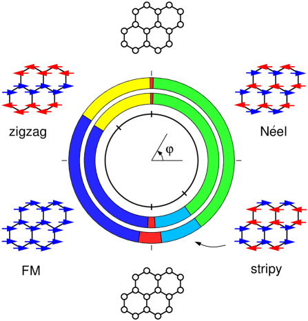
Figure 3: T$=0$ phase diagram for KH model. The outer ring is composed from ED data for the 24-site cluster, reproducing the result from Ref. Cha13 in the new parametrization, the middle ring shows CMFT results also for 24-site cluster and the inner black circle represents the classical result. The convention used for the angular parameter $\varphi$ which determines coupling constants [see Eqs. (2) and (3)] is shown in the center of the inner circle. The colors represent particular phases, shown also as mini-drawings next to suitable regions of the phase diagram. Starting from $\varphi=0$ green colored region corresponds to Néel order, red — KSL, yellow — zigzag order, dark blue — FM, red — KSL, light blue — stripy phase and again green — Néel phase.

It is clearly visible that all the methods that include quantum fluctuations give quantum versions of the four classically established magnetic phases: Néel, zigzag, FM and stripy. As the most important effect we note that when quantum fluctuations are included within a classical phase, the energy is generally lowered and that the emerging phase is expected to expand beyond the classical boundaries, but only in case if a phase which competes with it has weaker quantum fluctuations. This implies that phases of AF nature will expand at the expense of the FM ones as the latter phases have lower energy gains by quantum fluctuations (which even vanish exactly for the FM order at $K=0$ and $J<0$).

We summarize the phase boundaries obtained within different methods in Table 1. One finds substantial corrections to the quantum phase transitions which follow from quantum fluctuations. These corrections are quite substantial in both KSLs at the Kitaev points ($K=+1$, $\varphi=\frac{1}{2}\pi$ and $K=-1$, $\varphi=\frac{3}{2}\pi$, first column of Table 1). Indeed, in the classical approach massively degenerate ground states exist just at isolated points but they are replaced by disordered spin-liquid states that extend to finite intervals of $\varphi$ when quantum fluctuations are included, see the second, third and fourth column in Table 1. The expansion of Néel and zigzag phases beyond classical boundaries is given by particularly large corrections and is well visible.

The most prominent feature in the phase diagram described above is however the difference in size between two KSL regions, already addressed before using ED Cha13 and also visible now in the CMFT data. Therefore, the CMFT result supports the claim from Ref. Cha13 that the stability of KSL perturbed by relatively small Heisenberg interaction depends on the nature of the phases surrounding the spin liquid and the amount of quantum fluctuations that they carry. In the following we discuss the above issues more thoroughly, examining: (i) ground state energy curves emerging from ED, CMFT, SOPT within the linked cluster expansion and LSW, (ii) the ordered moment given by various methods, (iii) the spin–spin correlation functions, and (iv) the spin structure factor as well as the dynamical spin susceptibility in the vicinity of the Kitaev points.

IV.2 Quantum corrections: energetics

We start the discussion of quantum corrections to the energy of the ordered phases by noting that, even though it properly captures finite order parameters, the CMFT looses quantum energy on the external bonds and does not therefore provide a reliable estimate of the ground-state energy. Instead, the energy obtained using the ED calculations [see Fig. 4(a)] will be treated as a reference value. This is supported by the fact that the ED phase boundaries were roughly confirmed by tensor networks (iPEPS) Ire14 and DMRG results Tre11 : While the iPEPS phase boundaries agree with ED for AF KSL/LRO transitions and the boundaries between different LRO phases differ only slightly from those found in ED (iPEPS: zigzag/FM – $0.808\pi$, stripy/Néel – $1.708\pi$), for FM KSL/LRO transition however the iPEPS result KSL/stripy – $1.528\pi$). On the other hand, DMRG boundaries agree perfectly with ED and due to four–sublattice dual transformation Kha05 ; Cha10 one can reproduce the FM/zigzag as well as FM/KSL boundaries. Only the extent of the AF spin-liquid phase cannot be extracted from this result, but that is already confirmed by iPEPS.

Table 1: Phase boundaries for KH model, parameterized by the angle $\varphi$ (in units of $\pi$), see Eqs. (2) and (3). Columns: classical Luttinger-Tisza approximation, second–order perturbation theory, exact diagonalization, and self–consistent cluster mean field theory.

boundary	classical	SOPT	ED	CMFT
Néel/KSL	$0.5$	$0.492$	$0.494$	$0.493$
KSL/zigzag	$0.5$	$0.507$	$0.506$	$0.505$
zigzag/FM	$0.75$	$0.813$	$0.814$	$0.825$
FM/KSL	$1.5$	$1.463$	$1.448$	$1.481$
KSL/stripy	$1.5$	$1.530$	$1.539$	$1.517$
stripy/Néel	$1.75$	$1.705$	$1.704$	$1.699$

Fig. 4(a) shows a quite remarkable agreement between the energy values and critical values of $\varphi$ obtained by the simplest SOPT Cha10 and our reference ED results. This suggests that this analytical method can be utilized to get better insight to the quantum contributions to the ground state energy. For the four phases with LRO, the energy per site ${\cal E}$, written as a sum of the classical energy $E_{\mathrm{class}}$ and the quantum fluctuation contribution $\Delta E$, is obtained as:

$${\cal E}_{\rm N} = -\frac{1}{8}(K+3J)-\frac{1}{16}(K+3J),$$ (11)

$${\cal E}_{\rm ZZ} = -\frac{1}{8}(K-J)-\frac{1}{16}(K-J),$$ (12)

$${\cal E}_{\rm FM} = +\frac{1}{8}(K+3J)+\frac{1}{16}\frac{K^{2}}{K+2J},$$ (13)

$${\cal E}_{\rm ST} = +\frac{1}{8}(K-J)+\frac{1}{16}\frac{(K+2J)^{2}}{K}.$$ (14)

In addition, to get the LRO/KSL phase boundary points in Table 1, we estimate the energy of the KSL phase as

$${\cal E}_{\rm KSL}\simeq\frac{3}{2}(K+J)\langle S^{\gamma}S^{\gamma}\rangle_{\mathrm{Kitaev}},$$ (15)

using the analytical result for the Kitaev points Bas07 , $\langle S^{\gamma}S^{\gamma}\rangle_{\mathrm{Kitaev}}\approx\pm 0.131$.

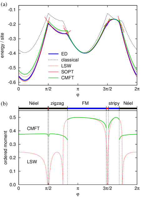
Figure 4: (a) Comparison between ground state energies per site obtained using various methods: classical Luttinger-Tisza approximation (dashed black), SOPT (solid red), LSW approximation (dashed red), ED for 24-site cluster (solid blue, see Cha13 for this result in a different parametrization), and CMFT (solid green). (b) Ordered moment value obtained from CMFT (green line) and LSW (dashed red line). For CMFT the values were obtained by averaging $\pm\langle S_{i}^{z}\rangle$ over the boundary sites, with the signs determined by the particular type of magnetic order.

The two spin-liquid phases in the phase diagram of KH model differ strongly in their extent, despite the formal equivalence of the FM and AF Kitaev points provided by an exact mapping of the Hamiltonian Kit06 . As mentioned earlier, this is due to the fact that the two KSLs compete with LRO phases of a distinct nature. Here we give a simple interpretation based on the strength of the quantum corrections of the LRO phases estimated using (11)–(14). Later, in Secs. V and VI we illustrate the different nature of the transitions between FM and AF KSL and the surrounding it LRO phases in terms of spin correlations and spin dynamics.

Let us now compare the quantum fluctuation contribution and the classical one. For the LRO phases surrounding the AF spin liquid — Néel and zigzag — we always have $\Delta E/E_{\mathrm{class}}=\frac{1}{2}$ as deduced from Eqs. (11) and (12), i.e., only $\frac{2}{3}{\cal E}_{\rm N}$ and $\frac{2}{3}{\cal E}_{\rm ZZ}$ are found in the classical approach. This guarantees that the quantum phase transition between these two types of order occurs at the same value of $\varphi=\pi/2$ in SOPT and in the classical approach that do not capture the spin-liquid phase in between these ordered states, see Fig. 4(a). In contrast, the phases neighboring to the FM spin liquid — FM and stripy — would reach the value of $\Delta E/E_{\mathrm{class}}=\frac{1}{2}$ only at the FM Kitaev point with $J=0$ and away from this point the contribution of quantum fluctuations decreases rapidly allowing for large extent of the FM spin-liquid phase. Note, that both these latter phases contain a point which is exactly fluctuation free — for FM phase when frustration is absent ($K=0$), and for stripy phase it is related to the FM one by the interaction transformation Cha15 at $K=-2J$.

Moving to the CMFT energy analysis (green line in Fig. 4(a)) one should also keep in mind that within the CMFT method the external bonds between $\langle S^{z}_{i}\rangle$ and $S^{z}_{j}$ do not include quantum fluctuations fully. This implies worse estimate of the energy for regions of the phase space that allow quantum fluctuations. As a consequence the region of stability of FM spin-liquid phase is smaller than that obtained in the ED. Finally, the estimates obtained from LSW, which represents a harmonic approximation to the quantum fluctuations, are typically better than those from the CMFT but not as good as those from SOPT, see dashed red lines in Fig.  4(a). As expected, the LSW energy fits well with ED curve for FM and stripy phases with less quantum fluctuations and starts to diverge when beyond quantum phase transitions within Néel and zigzag phases.

IV.3 Quantum corrections: ordered moment

As usual, getting the correct value of the ordered moment turns out to be a more difficult task than estimating the ground state energy. This is primarily due to the fact that the ED does not capture the symmetry-broken states and the ordered moment can only be indirectly extracted from the $m^{2}$; moreover, the SOPT may not be reliable here. Hence, we are mostly left with the results obtained with CMFT and LSW. We discuss the corresponding data [shown in Fig. 4(b)] together with the several values given already in the literature.

Let us begin with the Heisenberg AF point $\varphi=0$: here it is expected that the ordered moment should be strongly reduced by quantum fluctuations. LSW approximation estimates the ordered moment value at $0.248$ Wei91 . Similar values were extracted from $m^{2}$ in quantum Monte Carlo ($0.268$ Reg89 ; Cas06 ; Low09 ) and ED calculations ($0.270$ Alb11 ). In the last case however the authors admit that the set of clusters for finite size scaling was chosen so as to make the best agreement with quantum Monte Carlo. Another method — series expansion (high order perturbation theory) Oit15 sets ordered moment value at a somewhat higher value of $0.307$. While all the above results seem roughly consistent, CMFT value seems to stand out ($0.374$ for $\varphi=0$). Nevertheless, one should note that the ordered moment estimated from $m^{2}$ for 24–site cluster ED equals $0.45$ Alb11 which is above the CMFT value. This suggests that at this point the finite size scaling is important.

Before transferring to the frustrated regime we briefly mention that the the trivial ordered moment value at $\varphi=\pi$ is here correctly reproduced by both CMFT and LSW. Besides, for the regions around the fluctuation–free FM (and stripy) point the ordered moments predicted by CMFT and LSW also match. Following the ground state energy analysis, LSW gives the correct result because quantum fluctuations contribution is small compared to the classical state. The further we move towards the Kitaev points, however, the more incorrect the LSW approximation should be because of the strong reduction of the ordered moment due to the growing frustration.

In contrast, the lack of quantum fluctuations on the external bonds makes CMFT steadily biased except for FM and stripy phases. However, since for the internal part of the cluster the fluctuations are still fully included, the frustration should be well handled and CMFT should give more predictable results than LSW in frustrated parts of the phase diagram. Here it is also important to stress, that the series expansion captures correctly the fluctuation–free point at $\varphi=\pi$ (FM) and $\varphi=-\arctan 2$ (stripy) and predicts a broader region of FM KSL phase Oit15 . The order parameter is also qualitatively correctly estimated and is reduced more to $m\simeq 0.3$ for both Néel and zigzag phases Oit15 . However, while the ordered moment values obtained by CMFT are consistent with the four–sublattice dual transformation, the ordered moment data from the high–order perturbation theory Oit15 are not, as the ordered moment values differ at the points connected by the mapping. Unfortunately the largest difference appears near the FM LRO/KSL boundaries. This observation uncovers certain limits of the high–order perturbation theory.

IV.4 Quantum corrections: naive interpretation

Let us conclude the discussion of the quantum corrections with the following more general observation: Developing the argumentation presented by Iregui, Corboz, and Troyer Ire14 , the dependence of the quantum correction to the energy and to the ordered moment on the angle $\varphi$ suggests that the Kitaev interaction is less “compatible” with the FM/stripy ground states than with the Néel/zigzag ones. This can be understood in the simple picture of the KH model on a 4-site segment of the honeycomb lattice consisting of three bonds attached to a selected lattice site, as presented below.

Starting with $\varphi=\pi$ (FM ground state. e.g. along the $z$ quantization axis) and increasing $\varphi$ leads to an addition of the FM Kitaev term, which favors FM-aligned spins along the $x$, $y$, and $z$ quantization axes for the $x$, $y$, and $z$ directional bonds, respectively. It can easily be seen that, e.g. for the $x$ bond, the eigenstate of the FM Kitaev-only Hamiltonian on that bond ($|\uparrow_{x}\uparrow_{x}\rangle$) has a $25\%$ overlap with the FM ground state, $|\langle\uparrow_{z}\uparrow_{z}|\uparrow_{x}\uparrow_{x}\rangle|^{2}=\frac{1}{4}$. In contrast, while a similar situation happens for the $y$ bond, for the $z$ bond there is a $100\%$ overlap between such states.

Next, we perform a similar analysis for $\varphi=0$ and firstly assume that we have a classical ground state. In this case for the “unsatisfied” bonds from the point of view of the increasing AF Kitaev interaction we also obtain that the eigenstate of the AF Kitaev-only Hamiltonian ($|\uparrow_{x}\downarrow_{x}\rangle$) on that bond has a $25\%$ overlap with the classical Néel ground state — e.g.: $|\langle\uparrow_{z}\downarrow_{z}|\uparrow_{x}\downarrow_{x}\rangle|^{2}=\frac{1}{4}$. However, this situation changes once we consider that the spin quantum fluctuations dress the classical Néel ground state. This can be best understood if we assumed the unrealistic but insightful case of very strong quantum fluctuations destroying the classical Néel ground state: then for the $x$ bond a singlet could be stabilized and the overlap between such a state and the state “favored” by the Kitaev term increases to $50\%$: $|\langle 0|\uparrow_{x}\downarrow_{x}\rangle|^{2}=\frac{1}{2}$. This suggests that the Néel ground state, which contains quantum spin fluctuations, is more “compatible” with the states “favored” by the Kitaev terms than the FM ground state, resulting in more stable values of ordered moment for Néel phase. It seems that the above difference is visible in CMFT data but not in LSW ones. We shall discuss this issue further by analyzing spin correlations below.

V Spin correlations

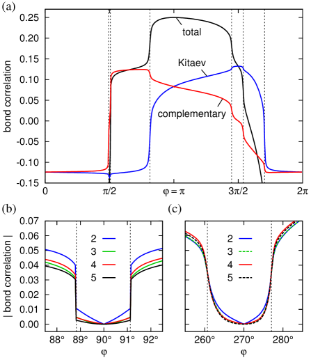
Figure 5: (a) Spin correlations $\langle\boldsymbol{S}_{i}\cdot\boldsymbol{S}_{j}\rangle$ obtained within ED for the bonds between nearest neighbors (black line), spin correlations of the components active in the Kitaev interaction, $\langle S^{\gamma}_{i}S^{\gamma}_{j}\rangle$ (blue line), and complementary spin components, $\langle S^{\bar{\gamma}}_{i}S^{\bar{\gamma}}_{j}\rangle$ (red line). Below further neighbor spin correlations $|\langle\boldsymbol{S}_{i}\cdot\boldsymbol{S}_{j}\rangle|$ are shown: (b) near the AF spin-liquid phase, and (c) for the angle $\varphi$ interval including the FM spin-liquid phase.

Additional information about the ground state is given by spin–spin correlation functions. In Fig.  5(a) one can observe isotropic stable $\langle S^{\gamma}_{i}S^{\gamma}_{j}\rangle$ correlations in almost the entire AF phase ($\langle\boldsymbol{S}_{i}\cdot\boldsymbol{S}_{j}\rangle\approx-0.36$ for $\varphi=0$), while for FM phase the anisotropy quickly develops when moving away from FM Heisenberg point $\varphi=\pi$ (here $\langle\boldsymbol{S}_{i}\cdot\boldsymbol{S}_{j}\rangle$ reaches the classical value $0.25$). This again demonstrates that the AF (and zigzag) phase is more robust and uniform than FM (and stripy) phase.

Moreover, spin-spin correlations allow us to confirm the disordered regions around the Kitaev points as critical cases of quantum spin liquid Tik11 . At the Kitaev points we observe the expected undisturbed KSL pattern: non–zero values of nearest neighbor correlations between spin components active in the Kitaev interaction (blue curve in Fig.  5(a)) and vanishing correlations between complementary components (red curve). In contrast, the next nearest and further neighbor correlations disappear, see Figs. 5(b) and 5(c). While moving away from the Kitaev points the absolute values of the correlations enter the regions of slow growth — these are signatures of the critical spin-liquid phases and they look similar in AF and FM spin liquid cases. At some point however proceeding further results in rapidly growing absolute values which mark KSL/LRO boundaries.

Furthermore, Figs. 5(b) and 5(c) prove that there is a qualitative difference between the two spin-liquid regimes. This is observed in the rapid growth of spin correlations at the onset of LRO: step-like jump visible in Fig. 5(b) contrasts with smoother crossover seen in Fig. 5(c). Below we investigate this distinct behavior by analyzing the dynamical spin susceptibility for various available phases. After Fourier transformation of the $z$–component correlations, we obtain the spin structure factor to be discussed in the context of the spin susceptibility also in Sec. VI.

VI Spin susceptibility and excitations in the vicinity of the Kitaev points

Below we study the spin dynamics within the KH model by analyzing the dynamical spin susceptibility at $T=0$,

$$\chi_{\alpha\alpha}(\boldsymbol{q},\omega)=i\int_{0}^{\infty}\left\langle\Phi_{0}|[S^{\alpha}_{\boldsymbol{q}}(t),S^{\alpha}_{-\boldsymbol{q}}(0)]\right|\Phi_{0}\rangle\,\mathrm{e}^{i\omega t}\,\mathrm{d}t,$$ (16)

with the Fourier-transformed spin operator defined via

$$S^{\alpha}_{\boldsymbol{q}}=\frac{1}{\sqrt{N}}\sum_{\boldsymbol{R}}\mathrm{e}^{-i\boldsymbol{q}\cdot\boldsymbol{R}}S^{\alpha}_{\boldsymbol{R}}\;$$ (17)

and $|\Phi_{0}\rangle$ denoting the cluster ground state. For $\omega>0$, the imaginary part of $\chi(\boldsymbol{q},\omega)$ reads as

$$\chi^{\prime\prime}_{\alpha\alpha}(\boldsymbol{q},\omega)=-\mathrm{Im}\,\langle\mathrm{\Phi_{0}}|\,S^{\alpha}_{\boldsymbol{q}}\;\frac{1}{\omega+E_{\mathrm{GS}}-\mathcal{H}+i\delta}\;S^{\alpha}_{-\boldsymbol{q}}\,|\mathrm{\Phi_{0}}\rangle\;,$$ (18)

which can be conveniently expressed as a sum over the excited states $\{|\nu\rangle\}$,

$$\chi^{\prime\prime}_{\alpha\alpha}(\boldsymbol{q},\omega)=\pi\sum_{|\nu\rangle}|\langle\nu|S^{\alpha}_{-\boldsymbol{q}}|\Phi_{0}\rangle|^{2}\delta(\omega-E_{\mathrm{\nu}})\;,$$ (19)

where the excitation energy $E_{\nu}$ is measured relative to the ground state energy $E_{\mathrm{GS}}$. We have evaluated $\chi_{\alpha\alpha}(\boldsymbol{q},\omega)$ by ED on a hexagonal cluster of $N=24$ sites. In the ED approach, the exact ground state of the cluster $|\Phi_{0}\rangle$ is found by Lanczos diagonalization, the operator $S^{\alpha}_{-\boldsymbol{q}}$ is applied, and the average of the resolvent $1/(z-\mathcal{H})$ is determined by Lanczos method using normalized $S^{\alpha}_{-\boldsymbol{q}}|\Phi_{0}\rangle$ as a starting vector Ful95 .

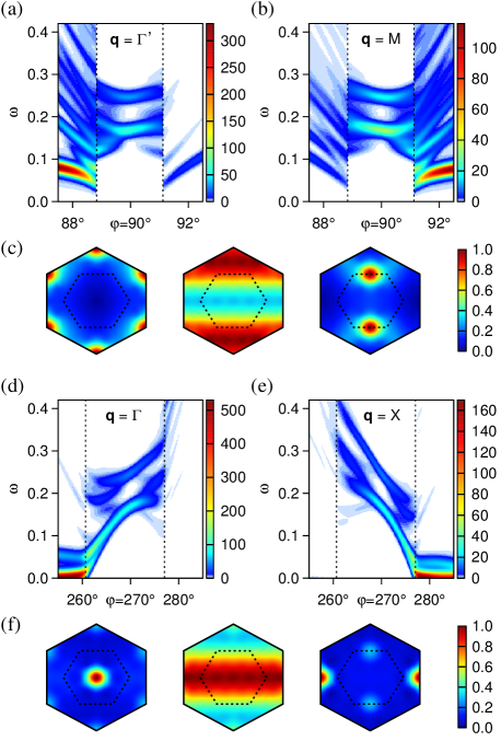
Figure 6: (a) Dynamical spin susceptibility $\chi^{\prime\prime}(\boldsymbol{q},\omega)$ obtained by ED near the AF KSL phase at the characteristic wavevector of the AF order, $\boldsymbol{q}=\Gamma^{\prime}$. (b) The same for the zigzag wavevector $\boldsymbol{q}=M$. (c) Brillouin zone portraits of the spin-structure factor $\langle S^{z}_{-\boldsymbol{q}}S^{z}_{\boldsymbol{q}}\rangle$ at $\varphi=87.5^{\circ}$, $90^{\circ}$, and $92.5^{\circ}$ (interpolated from the ED data). The inner hexagon is the Brillouin zone of the honeycomb lattice, the outer one corresponds to the triangular lattice with the missing sites filled in. (d,e) The same as in panels (a,b) but for the interval containing the FM ($\boldsymbol{q}=\Gamma$) and stripy ($\boldsymbol{q}=X$) phase. (f) Brillouin zone portraits of the spin-structure factor obtained at $\varphi=255^{\circ}$, $270^{\circ}$, and $285^{\circ}$.

In our case of the KH model, the calculation generally requires a relatively large number of Lanczos steps (up to one thousand) to achieve convergence of the dense high-energy part of the spectrum. Having the advantage of being exact, the method is limited by the $\boldsymbol{q}$ vectors accessible for a finite cluster and compatible with the PBC, and by finite-size effects due to small $N$. These concern mainly the low-energy part of $\chi^{\prime\prime}$ and lead e.g. to an enlarged gap of spin excitations in LRO phases of AF nature. Nevertheless, a qualitative understanding can still be obtained.

The evolution of numerically obtained $\chi^{\prime\prime}$ with varying $\varphi$ is presented in Figs. 6(a) and 6(b) for the region including AF spin-liquid phase, as well as in Figs. 6(d) and 6(e) for the region including the FM spin-liquid phase. The transitions are well visible at the characteristic $\boldsymbol{q}$ vectors of the individual LRO phases. The structure factor pattern, see Figs. 6(c) and 6(f), changes accordingly between the sharply peaked one in LRO phases and a wave-like form characteristic for nearest neighbor correlations in the spin-liquid phases.

After entering the spin-liquid phase, further changes of the spin response are very different for the AF and FM case. In the AF case, there is a sharp transition — a level crossing at our cluster, so that the ground state changes abruptly. The original intense pseudo-Goldstone mode as well as many other excited states become inactive in the spin-liquid phase. The observed low–energy gap in $\chi^{\prime\prime}$ varies only slightly with $\varphi$.

In contrast, when entering the FM spin-liquid phase the excitation that used to be the gapless magnon mode is characterized by a gradually increasing gap which culminates at the Kitaev point. Starting from the Kitaev point, the gradual reduction of the low–energy gap in $\chi^{\prime\prime}$ due to the Heisenberg perturbation manifests itself by a development of spin correlations beyond nearest neighbors (already reported in Fig. 2 of Ref. Cha10 ) and an increase of the static susceptibility to the magnetic field Zeeman-coupled to the order parameter of the neighboring LRO phase. This susceptibility then diverges at the transition point (see also Fig. 3 of Ref. Cha10 ).

VII Summary and conclusions

In the present paper we studied the phase diagram of the Kitaev-Heisenberg model by a combination of exact diagonalization and cluster mean field theory (CMFT), supplemented by the insights from linear spin-wave theory and the second–order perturbation theory. Both methods allowed to stabilize previously known ordered phases: Néel, zigzag, FM and stripy. Moreover, the ordered moment analysis provided by cluster mean field approach demonstrates Néel–zigzag and FM–stripy connections described before Cha13 . Compared to the previous CMFT studies utilizing $N=6$ site cluster (see Ref. Got15 or the Appendix), we have used a sufficiently large cluster of $N=24$ sites preserving the lattice symmetries and improving the ratio between internal and boundary bonds. This led to a balanced approach which allowed us to treat both ordered and disordered (spin-liquid) states on equal footing.

As the main result, the present study uncovers a fundamental difference between the onset of broken symmetry phases in the vicinity of Kitaev points with antiferromagnetic or ferromagnetic interactions. While the spin liquids obtained at $K=+1$ and $K=-1$ are strictly equivalent and can be transformed one into the other in the absence of Heisenberg interactions (at $J=0$), spin excitations and quantum phase transitions emerging at finite $J$ are very different in both cases. For antiferromagnetic Kitaev spin liquid phase ($K\simeq 1$) one finds that a gap opens abruptly in $\chi^{\prime\prime}(\boldsymbol{q},\omega)$ at $\boldsymbol{q}=\Gamma^{{}^{\prime}}$ and $\boldsymbol{q}=M$ when the ground state changes to the critical Kitaev quantum spin liquid. This phase transition is abrupt and occurs by level crossing. In contrast, for ferromagnetic spin liquid $K\simeq-1$ the gaps in $\chi^{\prime\prime}(\boldsymbol{q},\omega)$ at $\boldsymbol{q}=\Gamma$ and $\boldsymbol{q}=X$ open gradually from the points of quantum phase transition from ordered to disordered phase. With much weaker quantum corrections for ordered phases in the regime of ferromagnetic Kitaev interactions, the spin liquid is more robust near $K=-1$ as a phase that contains quantum fluctuations and survives in a broader regime than near $K=1$ when antiferromagnetic Kitaev interactions are disturbed by increasing (antiferromagnetic or ferromagnetic) Heisenberg interactions. This behavior is reminiscent of the ferromagnetic Kitaev model in a weak magnetic field Tik11 .

Appendix A Comparison between CMFT and linearized CMFT for a single hexagon

Here we compare linearization results for a single hexagon with full CMFT to see how well linearized CMFT performs as a shortcut method. It is important to realize that this cluster is not compatible with stripy or zigzag order because of their four-site magnetic unit cell, see Fig. 1(b), and they are suppressed within vast regions of $\varphi$ compared to the 24-site case. The size of the system allows for quick CMFT computations and enables detailed comparison between the two approaches. Moreover, specific problems linked to the above incompatibility make the $N=6$-site cluster a good test case to illustrate the linearized CMFT.

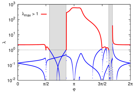
Figure 7: Full linearized CMFT result for a single hexagon. Blue lines represent all emerged positive eigenvalues $\lambda$, while maximal $\lambda$ larger than 1 is indicated in red.

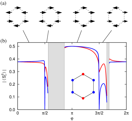
Figure 8: (a) Spin patterns obtained for a single hexagon by CMFT. From the left: Néel, zigzag, FM and stripy. (b) Phase diagram for a single hexagon determined by $|\langle S_{i}^{z}\rangle|$. Red and blue sites (see inset) are nonequivalent in the present CMFT due to the approximation given by Eq. (5) which generates the terms $\propto J$ that add to Kitaev term only on the vertical bonds $\langle ij\rangle\parallel z$ in the MF part of the Hamiltonian (1).

Following the procedure described in Sec. III.3, 6 eigenvalues $\lambda_{i}$ are produced for each value of $\varphi$ parameter. The corresponding spin patterns are inferred by inspecting the eigenvectors. Only the patterns associated with $\lambda_{i}>1$ are able to grow during iterations and eventually stabilize as a self-consistent solution of full CMFT. Comparison of both methods presented in Figs. 7 and 8 provides the phase diagram for a single hexagon: Néel phase for $\varphi\in[0,0.5)\pi$, KSL for $\varphi=\frac{\pi}{2}$, zigzag phase for $\varphi\in(0.5,0.555)\pi$, disordered region I for $\varphi\in(0.555,0.864)\pi$, FM phase for $\varphi\in(0.864,1.5)\pi$, KSL for $\varphi=\frac{3}{2}\pi$, stripy phase for $\varphi\in(1.5,1.62)\pi$ (linearization), $\varphi\in(1.5,1.64)\pi$ (CMFT), disordered region II for $\varphi\in(1.62,1.684)\pi$ (linearization) and $\varphi\in(1.64,1.684)\pi$ (CMFT), and Néel phase for $\varphi\in(1.684,2]\pi$. In contrast to $N=24$ cluster the two spin-liquid regions are replaced by single points $\varphi=\frac{\pi}{2}$ and $\varphi=\frac{3}{2}\pi$.

Striking difference between phase diagrams for 24-site and 6-site clusters is the reduction of the zigzag and stripy phases and the emergence of two regions of disorder indicated by two gray-shaded regions. Here all $\lambda_{i}<1$ and no spin pattern is strong enough to stabilize. Zigzag pattern emerges from CMFT with random initial values of $\langle S_{i}^{z}\rangle$ without additional help. Stripy pattern however is more difficult to catch. As one can see in Fig. 7, two different $\lambda_{i}$ corresponding to two stripy patterns exchange at $\varphi=1.568\pi$. Unfortunately, huge parasitic oscillations make these patterns extremely difficult to stabilize within CMFT. These stem from a large negative $\lambda_{i}$ that previously corresponded to FM pattern and decreased rapidly for $\varphi>1.5\pi$. If one recalls that the equivalent of one iteration in linearized version of CMFT is in fact multiplication by $\lambda_{i}$, one can easily see that large negative $\lambda_{i}$ would cause oscillations with an exponentially growing amplitude when performing the iterations of the self-consistent loop. To overcome this issue we introduce a damping into a self-consistent loop by taking $(1-d)\langle S_{i}^{z}\rangle_{\mathrm{fin}}+d\langle S_{i}^{z}\rangle_{\mathrm{ini}}$ as the new averages. Here $d<1$ is a suitably chosen damping factor. With this modification CMFT produces one finite stripy order suggested by linearization. However since the parasitic negative $\lambda_{i}$ grows enormously in magnitude as we approach the phase boundary an extreme damping has to be included making the phase boundary hard to determine by using CMFT.

In conclusion, it is evident that the ordered patterns suggested by linearization were reproduced by CMFT within regions dictated by the maximal $\lambda_{i}>1$. Moreover, the linearized procedure indicated possible difficulties with stabilizing stripy phases that had to be cured by a strong damping introduced into the self-consistent loop.

References

- (1) Bruce Normand, Cont. Phys. 50, 533 (2009).
- (2) Leon Balents, Nature (London) 464, 199 (2010).
- (3) L. Savary and L. Balents, arXiv:1601.03742 (2016).
- (4) G. Khaliullin and S. Maekawa, Phys. Rev. Lett. 85, 3950 (2000); G. Khaliullin, P. Horsch, and A. M. Oleś, ibid. 86, 3879 (2001).
- (5) A. B. Harris, T. Yildirim, A. Aharony, O. Entin-Wohlman, and I. Ya. Korenblit, Phys. Rev. Lett. 91, 087206 (2003).
- (6) M. Daghofer, K. Wohlfeld, A. M. Oleś, E. Arrigoni, and P. Horsch, Phys. Rev. Lett. 100, 066403 (2008); K. Wohlfeld, M. Daghofer, A. M. Oleś, and P. Horsch, Phys. Rev. B 78, 214423 (2008).
- (7) M. Daghofer, A. Nicholson, A. Moreo, and E. Dagotto, Phys. Rev. B 81, 014511 (2010); A. Nicholson, W. Ge, X. Zhang, J. Riera, M. Daghofer, A. M. Oleś, G. B. Martins, A. Moreo, and E. Dagotto, Phys. Rev. Lett. 106, 217002 (2011).
- (8) P. Wróbel and A. M. Oleś, Phys. Rev. Lett. 104, 206401 (2010); P. Wróbel, R. Eder, and A. M. Oleś, Phys. Rev. B 86, 064415 (2012).
- (9) S. Di Matteo, G. Jackeli, C. Lacroix, and N. B. Perkins, Phys. Rev. Lett. 93, 077208 (2004); S. Di Matteo, G. Jackeli, and N. B. Perkins, Phys. Rev. B 72, 024431 (2005).
- (10) G. Khaliullin, Prog. Theor. Phys. Suppl. 160, 155 (2005).
- (11) G. Jackeli and D.A. Ivanov, Phys. Rev. B 76, 132407 (2007).
- (12) G. Jackeli and D.I. Khomskii, Phys. Rev. Lett. 100, 147203 (2008).
- (13) F. Krüger, S. Kumar, J. Zaanen, and J. van den Brink, Phys. Rev. B 79, 054504 (2009).
- (14) Gia-Wei Chern and N. Perkins, Phys. Rev. B 80, 220405(R) (2009).
- (15) A. van Rynbach, S. Todo, and S. Trebst, Phys. Rev. Lett. 105, 146402 (2010).
- (16) F. Trousselet, A. Ralko, and A. M. Oleś, Phys. Rev. B 86, 014432 (2012).
- (17) G. Chen and L. Balents, Phys. Rev. Lett. 110, 206401 (2013).
- (18) M. Daghofer, A. M. Oleś, and W. von der Linden, Phys. Rev. B 70, 184430 (2004).
- (19) A. Reitsma, L. F. Feiner, and A. M. Oleś, New J. Phys. 7, 121 (2005).
- (20) W. Witczak-Krempa, G. Chen, Y. B. Kim, and L. Balents, Annu. Rev. Condens. Matter Phys. 5, 57 (2014).
- (21) W. Brzezicki, A. M. Oleś, and M. Cuoco, Phys. Rev. X 5, 011037 (2015); W. Brzezicki, M. Cuoco, and A. M. Oleś, J. Supercond. Novel Magn. 29, 563 (2016).
- (22) G. Jackeli and G. Khaliullin, Phys. Rev. Lett. 102, 017205 (2009).
- (23) A. Kitaev, Ann. Phys. (N.Y.) 321, 2 (2006).
- (24) G. Baskaran, S. Mandal, and R. Shankar, Phys. Rev. Lett. 98, 247201 (2007).
- (25) J. Chaloupka, G. Jackeli, and G. Khaliullin, Phys. Rev. Lett. 105, 027204 (2010).
- (26) Y. Singh and P. Gegenwart, Phys. Rev. B 82, 064412 (2010); F. Trousselet, G. Khaliullin, and P. Horsch, ibid. 84, 054409 (2011).
- (27) X. Liu, T. Berlijn, W.-G. Yin, W. Ku, A. Tsvelik, Y.-J. Kim, H. Gretarsson, Y. Singh, P. Gegenwart, and J. P. Hill, Phys. Rev. B 83, 220403(R) (2011).
- (28) Y. Singh, S. Manni, J. Reuther, T. Berlijn, R. Thomale, W. Ku, S. Trebst, and P. Gegenwart, Phys. Rev. Lett. 108, 127203 (2012).
- (29) S. K. Choi, R. Coldea, A. N. Kolmogorov, T. Lancaster, I. I. Mazin, S. J. Blundell, P. G. Radaelli, Y. Singh, P. Gegenwart, K. R. Choi, S.-W. Cheong, P. J. Baker, C. Stock, and J. Taylor, Phys. Rev. Lett. 108, 127204 (2012).
- (30) F. Ye, S. Chi, H. Cao, B. C. Chakoumakos, J. A. Fernandez-Baca, R. Custelcean, T. F. Qi, O. B. Korneta, and G. Cao, Phys. Rev. B 85, 180403 (2012).
- (31) R. Comin, G. Levy, B. Ludbrook, Z.-H. Zhu, C. N. Veenstra, J. A. Rosen, Y. Singh, P. Gegenwart, D. Stricker, J. N. Hancock, D. van der Marel, I. S. Elfimov, and A. Damascelli, Phys. Rev. Lett. 109, 266406 (2012).
- (32) H. Gretarsson, J. P. Clancy, X. Liu, J. P. Hill, E. Bozin, Y. Singh, S. Manni, P. Gegenwart, J. Kim, A. H. Said, D. Casa, T. Gog, M. H. Upton, H.-S. Kim, J. Yu, V. M. Katukuri, L. Hozoi, J. van den Brink, and Y.-J. Kim, Phys. Rev. Lett. 110, 076402 (2013).
- (33) F. Trousselet, M. Berciu, A. M. Oleś, and P. Horsch, Phys. Rev. Lett. 111, 037205 (2013).
- (34) J. Chaloupka, G. Jackeli, and G. Khaliullin, Phys. Rev. Lett. 110, 097204 (2013).
- (35) V. M. Katukuri, S. Nishimoto, V. Yushankhai, A. Stoyanova, H. Kandpal, S. Choi, R. Coldea, I. Rousochatzakis, L. Hozoi, and J. van den Brink, New. J. Phys. 16, 013056 (2014).
- (36) S. M. Winter, Y. Li, H. O. Jeschke, and R. Valentí, Phys. Rev. B 93, 214431 (2016).
- (37) F. Trousselet, P. Horsch, A. M. Oleś, and W.-L. You, Phys. Rev. B 90, 024404 (2014).
- (38) S. H. Chun, J.-W. Kim, J. Kim, H. Zheng, C. C. Stoumpos, C. D. Malliakas, J. F. Mitchell, K. Mehlawat, Y. Singh, Y. Choi, T. Gog, A. Al-Zein, M. Moretti Sala, M. Krisch, J. Chaloupka, G. Jackeli, G. Khaliullin, and B. J. Kim, Nature Physics 11, 462 (2015).
- (39) J. Chaloupka and G. Khaliullin, Phys. Rev. B 92, 024413 (2015).
- (40) J. G. Rau and H. Y. Kee, arXiv:1408.4811 (2014).
- (41) A. Banerjee, C. A. Bridges, J.-Q. Yan, A. A. Aczel, L. Li, M. B. Stone, G. E. Granroth, M. D. Lumsden, Y. Yiu, J. Knolle, S. Bhattacharjee, D. L. Kovrizhin, R. Moessner, D. A. Tennant, D. G. Mandrus, and S. E. Nagler, Nat. Mat. 15, 733 (2016).
- (42) A. F. Albuquerque, D. Schwandt, B. Hetényi, S. Capponi, M. Mambrini, and A. M. Laüchli, Phys. Rev. B 84, 024406 (2011).
- (43) D. C. Cabra, C. A. Lamas, and H. D. Rosales, Phys. Rev. B 83, 094506 (2011); A. Kalz, M. Arlego, D. Cabra, A. Honecker, and G. Rossini, ibid. 85, 104505 (2012); H. D. Rosales, D. C. Cabra, C. A. Lamas, P. Pujol, and M. E. Zhitomirsky, ibid. 87, 104402 (2013).
- (44) X. Y. Song, Y. Z. You, and L. Balents, Phys. Rev. Lett. 117, 037209 (2016).
- (45) J. G. Rau, Eric Kin-Ho Lee, and H. Y. Kee, Phys. Rev. Lett. 112, 077204 (2014).
- (46) J. Oitmaa, Phys. Rev. B 92, 020405(R) (2015).
- (47) H.-C. Jiang, Z.-C. Gu, X.-L. Qi, and S. Trebst, Phys. Rev. B 83, 245104 (2011); J. Reuther, R. Thomale, and S. Trebst, ibid. 84, 100406 (2011); I. Kimchi and Y. Z. You, ibid. 84, 180407 (2011); R. Schaffer, S. Bhattacharjee, and Y. B. Kim, ibid. 86, 224417 (2012); Y. Yu, L. Liang, Q. Niu, and S. Qin, ibid. 87, 041107 (2013); E. Sela, H.-C. Jiang, M. H. Gerlach, and S. Trebst, ibid. 90, 035113 (2014).
- (48) J. Osorio Iregui, P. Corboz, and M. Troyer, Phys. Rev. B 90, 195102 (2014).
- (49) K. Li, S.-L. Yu, and J.-X. Li, New J. Phys. 17, 043032 (2015).
- (50) M. Becker, M. Hermanns, B. Bauer, M. Garst, and S. Trebst, Phys. Rev. B 91, 155135 (2015).
- (51) G. Jackeli and A. Avella, Phys. Rev. B 92, 184416 (2015).
- (52) I. Rousochatzakis, U. K. Rössler, J. van der Brink, and M. Daghofer, Phys. Rev. B 93, 104417 (2016).
- (53) W. Brzezicki, J. Dziarmaga, and A. M. Oleś, Phys. Rev. Lett. 109, 237201 (2012); Phys. Rev. B 87, 064407 (2013); W. Brzezicki and A. M. Oleś, Phys. Rev. B 83, 214408 (2011).
- (54) D. Gotfryd and A. M. Oleś, Acta Phys. Polon. A 127, 318 (2015).
- (55) K. Foyevtsova, H. O. Jeschke, I. I. Mazin, D. I. Khomskii, and R. Valentí, Phys. Rev. B 88, 035107 (2013).
- (56) V. M. Katukuri, S. Nishimoto, V. Yushankhai, A. Stoyanova, H. Kandpal, S. Choi, R. Coldea, I. Rousochatzakis, L. Hozoi and J. van den Brink, New J. Phys. 16, 013056 (2015).
- (57) L. R. Walker, Spin Waves and Other Magnetic Modes in Magnetism (Academic Press, New York and London, 1963).
- (58) M. Raczkowski and A. M. Oleś, Phys. Rev. B 66, 094431 (2002).
- (59) P. A. Maksimov and A. L. Chernyshev, Phys. Rev. B 93, 014418 (2016).
- (60) Zheng Weihong, J. Oitmaa, and C. J. Hamer, Phys. Rev. B 44, 11869 (1991).
- (61) J. D. Reger, J. A. Riera, and A. P. Young, J. Phys.: Condens. Matter 1, 1855 (1989).
- (62) E. V. Castro, N. M. R. Peres, K. S. D. Beach, and A. W. Sandvik, Phys. Rev. B 73, 054422 (2006).
- (63) U. Löw, Condens. Matter Phys. 12, 497 (2009).
- (64) K. S. Tikhonov, M. V. Feigel’man, and A. Yu. Kitaev, Phys. Rev. Lett. 106, 067203 (2011).
- (65) P. Fulde, Electron Correlations in Molecules and Solids, Springer Series in Solid-State Sciences, Vol. 100 (Springer-Verlag, Berlin/Heidelberg/New York, 1995).