CGC factorization for forward particle production in proton-nucleus collisions at next-to-leading order

Abstract

Within the Color Glass Condensate effective theory, we reconsider the next-to-leading order (NLO) calculation of the single inclusive particle production at forward rapidities in proton-nucleus collisions at high energy. Focusing on quark production for definiteness, we establish a new factorization scheme, perturbatively correct through NLO, in which there is no ‘rapidity subtraction’. That is, the NLO correction to the impact factor is not explicitly separated from the high-energy evolution. Our construction exploits the skeleton structure of the (NLO) Balitsky-Kovchegov equation, in which the first step of the evolution is explicitly singled out. The NLO impact factor is included by computing this first emission with the exact kinematics for the emitted gluon, rather than by using the eikonal approximation. This particular calculation has already been presented in the literature Chirilli:2011km ; Chirilli:2012jd , but the reorganization of the perturbation theory that we propose is new. As compared to the proposal in Chirilli:2011km ; Chirilli:2012jd , our scheme is free of the fine-tuning inherent in the rapidity subtraction, which might be the origin of the negativity of the NLO cross-section observed in previous studies.

1 Introduction

Using perturbative QCD, we would like to study particle production in high-energy proton-nucleus ($pA$) collisions in the kinematical regime where the produced particle is semi-hard to hard (meaning that its transverse momenta can be larger than the nuclear saturation momentum $Q_{s}$, but not much larger) and it propagates at forward rapidity in the proton fragmentation region (that is, it makes a very small angle w.r.t. the collision axis) Kovchegov:1998bi ; Kovchegov:2001sc ; Dumitru:2002qt ; Albacete:2003iq ; Kharzeev:2003wz ; Iancu:2004bx ; Blaizot:2004wu ; Blaizot:2004wv ; Dumitru:2005gt ; Albacete:2010bs ; Tribedy:2011aa ; Rezaeian:2012ye ; Lappi:2013zma .

What is special about this kinematics is that the scattering probes the small-$x$ part of the nuclear wavefunction, but the large-$x$ part of the proton wavefunction, so it acts as a clean probe of the nuclear gluon distribution in the interesting regime where one expects large gluon occupation numbers and strong non-linear phenomena, like gluon saturation. This probe is ‘clean’ since the large-$x$ part of the proton wavefunction is very dilute and hence well described by the standard QCD parton picture and the associated collinear factorization. Accordingly, the overall process can be depicted as follows: a collinear parton from the proton undergoes multiple scattering off the dense gluon system in the nuclear target and hence acquires some transverse momentum $k_{\perp}$, before eventually fragmenting into the hadrons that are measured in the final state.

The above physical picture naturally lends itself to a hybrid factorization scheme Dumitru:2002qt ; Dumitru:2005gt for the calculation of the single-inclusive hadron multiplicity, which combines the collinear factorization for the parton distribution of the incoming proton and also for the fragmentation of the produced quark or gluon Ellis:1991qj , with the CGC factorization for the high-energy scattering between the collinear parton and the nucleus. The ‘CGC’ refers to the Color Glass Condensate effective theory, which is the appropriate pQCD framework to address the problem of high-energy scattering in the presence of high gluon densities Iancu:2002xk ; Iancu:2003xm ; Gelis:2010nm ; Kovchegov:2012mbw . This is essentially a theory for the gauge-invariant correlations of Wilson lines and their evolution with increasing energy. A Wilson line (a unitary matrix in the color group SU$(N_{c})$) is the $S$-matrix of an energetic parton which undergoes multiple scattering off a strong color field representing the gluon distribution of the target. The CGC factorization for ‘dilute-dense’ scattering associates one such a Wilson line to each of the partons partaking in the collision, separately in the direct amplitude and the complex conjugate amplitude. Cross-sections are obtained by averaging over all the configurations of the color fields in the target, a procedure which generates the Wilson-line correlators aforementioned. In the simplest case, that is for single-inclusive particle production at leading order, this correlator involves the trace of the product of two Wilson lines, which can be identified with the elastic $S$-matrix of a color dipole which scatters off the nuclear target.

Whereas this hybrid factorization may indeed look natural, in view of the underlying physical picture, its foundation in pQCD is not obvious, nor easy to establish. In order to make sense beyond tree-level, this scheme must be consistent with the QCD radiative corrections and notably with the collinear and high-energy evolutions. As we shall shortly explain, this issue is already non-trivial at leading-order (LO) and it becomes even more so at next-to-leading order (NLO) and beyond.

The LO version of the hybrid factorization for single-inclusive hadron production Dumitru:2002qt ; Dumitru:2005gt includes the LO DGLAP evolution for the parton distribution in the proton and for the parton fragmentation in the final state. It furthermore includes the LO B-JIMWLK evolution of the dipole $S$-matrix. The B-JIMWLK (from Balitsky, Jalilian-Marian, Iancu, McLerran, Weigert, Leonidov and Kovner) equations Balitsky:1995ub ; JalilianMarian:1997jx ; JalilianMarian:1997gr ; Kovner:2000pt ; Iancu:2000hn ; Iancu:2001ad ; Ferreiro:2001qy form an infinite hierarchy of coupled equations which describes the non-linear evolution of the $n$-point correlations of the Wilson lines. (Operators with different number of Wilson lines couple under the evolution due to multiple scattering.) This hierarchy drastically simplifies in the limit of a large number of colors $N_{c}\gg 1$, in which expectation values of gauge-invariant operators factorize from each other. In that limit, the evolution of the dipole $S$-matrix is governed by a closed non-linear equation, known as the Balitsky-Kovchegov (BK) equation Balitsky:1995ub ; Kovchegov:1999yj .

A first subtle point, which arises already at LO, refers to the relation between the cross-section for parton-nucleus scattering on one hand, and the dipole scattering amplitude on the other hand. In general, cross-sections and amplitudes are different quantities (e.g. they have different analytic properties) and it is only due to the high-energy approximations — notably, due to the fact that the high-energy amplitudes are purely absorptive — that such an identification becomes possible in the problem at hand. Yet, the consistency between this relation and the high-energy evolution is far from being trivial (see the discussion in Mueller:2012bn ). So far, this has been demonstrated up to next-to-leading order Kovchegov:2001sc ; Mueller:2012bn and there is no obvious reason why it should remain true in higher orders.

With this in mind, we can address the calculation of single-inclusive hadron production in $pA$ collisions at NLO. The NLO version of the DGLAP equation is known since long (see e.g. the textbook Ellis:1991qj for a pedagogical discussion). Recently, the BK equation and the full B-JIMWLK hierarchy have been promoted to NLO accuracy as well Balitsky:2008zza ; Balitsky:2013fea ; Kovner:2013ona . By itself, the NLO approximation turns out to be unstable Avsar:2011ds ; Lappi:2015fma ; Iancu:2015vea , due to the presence of large NLO corrections enhanced by transverse logarithms. A similar difficulty was already encountered for the NLO version of the BFKL equation (the linearized version of the BK equation valid when the scattering is week; see e.g. the textbook Kovchegov:2012mbw ). As in that case Kwiecinski:1997ee ; Salam:1998tj ; Ciafaloni:1999yw ; Altarelli:1999vw ; Ciafaloni:2003rd ; Vera:2005jt , resummation schemes have been devised also for the non-linear, BK and B-JIMWLK, equations Beuf:2014uia ; Iancu:2015vea ; Iancu:2015joa ; Hatta:2016ujq , to restore the convergence of perturbation theory. In particular, the collinearly-improved BK equation Iancu:2015vea ; Iancu:2015joa , which resums to all orders the double-collinear logarithms together with a subset of the single-collinear logarithms and with the running coupling corrections, appears to be a convenient tool for the phenomenology Iancu:2015joa ; Albacete:2015xza . Moreover, the full NLO BK equation with collinear improvement has recently been shown to be stable and tractable via numerical methods Lappi:2016fmu .

Besides the NLO evolution, a calculation of the particle production to NLO accuracy must include an equally accurate version of the impact factor. The ‘impact factor’ refers to the partonic subprocess and for the present purposes can be simply defined as the cross-section for parton-nucleus scattering in the absence of any QCD evolution. For more clarity, from now on, we shall assume that the parton from the proton which participates in the collision is a quark.

At LO, the impact factor is simply the cross-section for the scattering between a bare quark and a nucleus or, equivalently, the $S$-matrix for a bare dipole. At NLO, the wavefunction of the incoming quark (or dipole) may contain an additional gluon, to be referred to as the ‘primary gluon’ in what follows. This gluon can be released in the final state (‘real correction’), or not (‘virtual correction’), but in any case its emission modifies the cross-section (or the dipole amplitude) w.r.t. to its LO value.

Since the kinematics of this primary gluon is integrated over, the corresponding correction to the impact factor is truly a one-loop effect. So far, this correction has been computed via two different approaches, Chirilli:2011km ; Chirilli:2012jd and respectively Altinoluk:2011qy ; Altinoluk:2014eka , with results which are quite difficult to compare with each other, but a priori look different at NLO accuracy. In what follows, we shall mostly refer to the NLO calculation in Refs. Chirilli:2011km ; Chirilli:2012jd . This is better suited for our new developments in this paper and this is also the context in which emerged the problem of the negativity of the cross-section Stasto:2013cha , which attracted our interest on this topic. But our general philosophy for attacking this problem is perhaps closer in spirit to that in Altinoluk:2014eka , in that it involves no subtraction for the ‘rapidity divergence’ (see below).

When performing the one-loop integration alluded to above, one should keep in mind that there are regions in phase-space that have already been included at LO, at least approximately, via the collinear and the high-energy evolutions. In the absence of physical cutoffs, these regions would generate logarithmic divergences. The physical cutoffs are truly needed when solving the evolution equations (they define the boundaries of the corresponding phase-space), but they can often be avoided when computing the NLO correction to the impact factor. Namely, one can directly subtract the would-be divergences by using a suitable ‘renormalization prescription’, tuned to match the resummation performed by the LO evolution equations. This is the strategy followed by the authors of Refs. Chirilli:2011km ; Chirilli:2012jd .

Specifically, Refs. Chirilli:2011km ; Chirilli:2012jd used dimensional regularization plus minimal subtraction to ‘remove’ the collinear divergences. This is a rather standard procedure in the context of the collinear factorization and relies on the fact that the collinear divergences can be factorized from the transverse integrations, as they refer to the renormalization of the integrated parton distributions and fragmentation functions.

Refs. Chirilli:2011km ; Chirilli:2012jd furthermore proposed a ‘plus’ prescription in order to subtract the ‘rapidity divergence’, i.e. the would-be divergence at $x\to 0$, where $x$ is the longitudinal momentum fraction of the primary gluon w.r.t. the incoming quark. This prescription is quite common in the context of the $k_{\perp}$-factorization at next-to-leading order (see e.g. Ivanov:2012iv and references therein) and its ‘non-linear’ extension to the CGC factorization may look natural. Recall however that, underlying this prescription, there is the strong assumption that cross-sections in perturbative QCD at high-energy can be factorized in rapidity. This assumption is highly non-trivial (and still unproven in the general case and beyond LO accuracy) because the perturbative corrections are truly non-local in rapidity. Accordingly, it is a priori not obvious that the small-$x$ divergence can be factorized from the high-energy evolution of the various scattering operators — the ‘dipole $S$-matrices’ which describe the eikonal scattering between the quark-gluon projectile and the target. This being said, we shall explicitly demonstrate in this paper that, via an appropriate reorganization of the perturbative corrections, one can indeed obtain such a factorized expression, valid to NLO, which involves the ‘plus’ prescription and agrees with the proposal in Refs. Chirilli:2011km ; Chirilli:2012jd . However, we shall also argue that the manipulations associated with this reorganization — namely, with the subtraction of the high-energy evolution from the NLO impact factor — involve a considerable amount of fine-tuning, which may be dangerous in practice.

This fine-tuning might be at the origin of the negativity problem observed in explicit numerical calculations based on the factorization scheme in Chirilli:2011km ; Chirilli:2012jd : the cross-section for single-inclusive particle production suddenly turns negative for transverse momenta slightly larger than the target saturation momentum $Q_{s}$ Stasto:2013cha ; Stasto:2014sea . Various proposals to circumvent this problem, by either introducing a cutoff in the rapidity subtraction scheme Kang:2014lha ; Xiao:2014uba ; Ducloue:2016shw , or via a more careful implementation of the kinematics Stasto:2014sea ; Altinoluk:2014eka ; Watanabe:2015tja , have managed to alleviate the problem (by pushing it to somewhat larger values of the transverse momentum), but without offering a fully satisfactory solution, at either conceptual or practical level (see also the discussion in the recent review paper Stasto:2016wrf ). Whereas high-energy approximations are expected to become less accurate at sufficiently large transverse momenta $k_{\perp}\gg Q_{s}$, we find it surprising that they fail already in the transition region towards saturation ($k_{\perp}\gtrsim Q_{s}$) — a region whose description is in fact the main focus of the CGC effective theory Iancu:2002xk ; Iancu:2003xm ; Gelis:2010nm ; Kovchegov:2012mbw .

This negativity problem encouraged us to reconsider the overall calculation from a new perspective and thus propose a new factorization scheme for the high-energy aspects of the problem. In presenting this proposal below, we shall restrict ourselves to quark production, that is, we shall ignore other partonic channels and also the fragmentation of the quark into hadrons in the final state. Also, we shall omit all the NLO corrections associated with the collinear resummation, i.e. the finite terms which remain after subtracting the collinear divergence. These terms can be unambiguously distinguished from those referring to the high-energy factorization Ducloue:2016shw and can be simply added to our final results.

Our main observations and new results can be summarized as follows:

(i) In our opinion, the negativity problem is most likely related to the severe fine-tuning inherent in the rapidity subtraction. The ‘fine-tuning’ refers to the delicate balance between the NLO corrections which are included in the evolution of the dipole $S$-matrix and those which are subtracted via the ‘plus’ prescription in order to construct the NLO correction to the impact factor. As we shall explain in detail in Sect. 3.5, this subtraction amounts to a reorganization of the perturbation theory which exploits the integral representation for the solution to the BK equation. Any approximation in solving this equation, as well as the subsequent approximations which are in practice needed to derive the ‘plus’ prescription, will lead to an imbalance between the large, ‘added’ and ‘subtracted’, contributions and thus possibly to unphysical results.

(ii) The ‘plus’ prescription is actually not needed: the would-be ‘rapidity divergence’ is truly cut off by physical mechanisms, namely by energy conservation for the ‘real’ corrections and by probability conservation for the ‘virtual’ ones. The role of the energy conservation in constraining the longitudinal phase-space for the primary emission is in fact well appreciated Stasto:2014sea ; Altinoluk:2014eka . This constraint has been used to cut off the soft divergence in Ref. Altinoluk:2014eka and to alleviate the negativity problem in the context of the ‘plus’ prescription in Ref. Watanabe:2015tja . The corresponding constraint on the ‘virtual’ corrections has not been discussed to our knowledge, so we shall devote an appendix to an explicit NLO calculation which demonstrates this. Specifically, in App. A we show that the ‘virtual’ corrections with very short lifetimes — outside the physical range for the ‘real’ corrections — mutually cancel each other. This result is in fact natural: the ‘real’ and ‘virtual’ corrections must have the same support in longitudinal phase-space, since they should combine with each other to ensure probability conservation.

(iii) To NLO accuracy, the calculation of the single-inclusive forward particle production in dilute-dense collisions can be given a different factorization, cf. Eq. (3.2), in which the small-$x$ logarithm associated with the primary gluon emission is not included in the high-energy evolution, but is implicitly kept within the impact factor. The latter includes the incoming quark and its (not necessarily soft) primary gluon, which together scatter off the gluon distribution in the nucleus and thus measure its high-energy evolution. This is the same picture as for the CGC calculation of di-hadron production Marquet:2007vb ; Albacete:2010pg ; Dominguez:2011wm ; Iancu:2013dta , except that the kinematics of the primary gluon is now integrated over and one must add the ‘virtual’ corrections.

(iv) In the limit where the primary gluon is soft and treated in the eikonal approximation, our general formula in Eq. (3.2) reduces to the integral representation (33) of the solution to rcBK. This is indeed the correct result for the quark multiplicity at LO. Vice-versa, our formula may be viewed as a generalization of the LO BK evolution in which the very first gluon emission (and that emission only) is treated beyond the eikonal approximation. In view of that, we expect our result for the cross-section to be positive semi-definite, albeit we have not been able to prove this explicitly.

(v) Our general formula (3.2) is probably too cumbersome to be used in practice, due to the complicated structure of the transverse and longitudinal integrations, which are entangled with each other. Fortunately though, the problem can be considerably simplified in the interesting regime where the transverse momentum $k_{\perp}$ of the produced quark is sufficiently hard, $k_{\perp}\gtrsim Q_{s}$. In that regime, the primary gluon is relatively hard as well, with a transverse momentum $p_{\perp}\sim k_{\perp}$ (see the discussion in Sect. 2.4). This allows us to replace $p_{\perp}\sim k_{\perp}$ within the rapidity variables in Eq. (3.2) and thus deduce a much simpler result, Eq. (3.3), which is of the same degree of difficulty as the formulae used within previous numerical simulations Zaslavsky:2014asa ; Stasto:2013cha ; Stasto:2014sea ; Watanabe:2015tja ; Ducloue:2016shw , while at the same time avoiding the rapidity subtraction and the associated fine-tuning.

(vi) To ensure the desired NLO accuracy of the overall scheme, the high-energy evolution of the color dipoles must be computed to NLO as well. In Sect. 3.4 we complete our factorization scheme by specifying the NLO corrections associated with the high-energy evolution. As we also explain there, the inclusion of the NLO evolution in the problem at hand is a priori problematic, for two reasons: (a) the evolution of a dense wavefunction, like a nucleus, is not known beyond leading-order, and (b) the strict NLO approximation is expected to be unstable, due to large corrections enhanced by collinear logarithms. We provide solutions to these problems by relating the target evolution to that of the dilute projectile, which is indeed known to NLO accuracy Balitsky:2008zza , including the all-order resummation of the collinear logarithms Iancu:2015vea ; Iancu:2015joa . This is furthermore discussed in Appendices B and C.

(vii) To make contact with the formalism in Chirilli:2011km ; Chirilli:2012jd , we consider in Sect. 3.5 the decomposition of our general result (3.3) between NLO dipole evolution and NLO corrections to the impact factor. This decomposition, shown in schematic notations in Eq. (45), relies in an essential way on the fact that the dipole $S$-matrix obeys a specific evolution equation — either the LO BK equation with running-coupling (rcBK) Kovchegov:2006wf ; Kovchegov:2006vj ; Balitsky:2006wa , or the NLO BK equation Balitsky:2008zza with collinear improvement Iancu:2015vea ; Iancu:2015joa , depending upon the desired accuracy. Indeed, the integral version of the evolution equation is used to reshuffle the largest contribution to the cross-section, that associated with the LO evolution.

Eq. (45) is very similar, but not fully identical, to the factorization scheme proposed in Chirilli:2011km ; Chirilli:2012jd , which is schematically shown in Eq. (46). As explained in Sect. 3.5, the differences between Eqs. (45) and (46) are irrelevant to NLO accuracy, but they can be nevertheless important in practice, as they introduce an imbalance between the terms included in the dipole evolution and those subtracted via the ‘plus’ prescription. As already mentioned at point (i), we believe that this imbalance is responsible for the problem of the negativity of the cross-section.

To summarize, all the potential difficulties with the subtraction method can be avoided by computing the cross-section directly from our formula (3.3), which involves no subtraction at all. This formula can be evaluated with a suitable approximation for the high-energy evolution, like rcBK or the more elaborated approximations described in Sect. 3.4 and in Appendix B.

This paper includes two major sections, devoted to the LO and the NLO calculations respectively, and three appendices. Sect. 2 starts with a discussion of the kinematics and of the importance of the choice of a Lorentz frame for building a physical picture. Such a picture is first developed in the target infinite momentum frame (in Sects. 2.1 and 2.2), then extended to a mixed frame, where one of the evolution gluons (the ‘primary gluon’) is viewed as an emission by the incoming quark, whereas all the subsequent ones are included in the evolution of the nuclear target (in Sect. 2.3). In Sect. 2.4, we discuss the di-jet configurations which control the final state in the regime where the produced quark has a large transverse momentum $k_{\perp}\gg Q_{s}$. The first subsection of Sect. 3 summarizes the result for the NLO impact factor obtained in Chirilli:2011km ; Chirilli:2012jd and also extends that result by specifying the rapidity variables for the evolution of the various dipole $S$-matrices. This discussion motivates our main result in this paper, that is, the NLO factorization displayed in Eq. (3.2). This general but rather cumbersome expression is rendered more tractable and also more explicit in Sects. 3.3, 3.4 and in Appendix B, where we simplify the kinematics via approximations appropriate at large $k_{\perp}\gtrsim Q_{s}$ and we replace the unknown NLO evolution of the nuclear target by that of the dilute quark-gluon projectile (with collinear improvement). In Sect. 3.5, we isolate LO from NLO contributions, as described at point (vii) above. Sect. 4 contains our conclusions. In Appendix A we demonstrate the mutual cancellation of the ‘virtual’ fluctuations whose lifetime is shorter than the longitudinal extent of the target. Finally, Appendices B and C give more details on the NLO evolution of color dipoles.

2 The leading order calculation

In this section, we shall briefly review the leading-order (LO) calculation of single-inclusive quark production in high-energy proton-nucleus ($pA$) at forward rapidities (i.e. in the proton fragmentation region). This calculation relies on a hybrid factorization scheme Dumitru:2005gt which involves collinear factorization at the level of the proton wavefunction together with the dipole picture for the scattering between a collinear quark from the proton and the nuclear gluon distribution.

2.1 General picture and kinematics

To LO in perturbative QCD and in a suitable Lorentz frame, the forward production of a quark in $pA$ collisions proceeds via the transverse momentum broadening of one of the quarks from the incoming proton: the quark, which was originally collinear with the proton, acquires a transverse momentum $\bm{k}$ via scattering off the small-$x$ gluons in the nuclear wavefunction and thus emerges at a small angle $\theta\simeq k_{\perp}/k^{+}$ w.r.t. the collision axis. The typical situation is such that the quark undergoes multiple soft scattering and thus accumulates a transverse momentum of order $Q_{s}$ — the target saturation momentum at the longitudinal resolution probed by the scattering (see below). But the $k_{\perp}$-distribution of the produced quark also features a power-like tail at high momenta $k_{\perp}\gg Q_{s}$, which is the result of a single, relatively hard, Coulomb scattering off the color sources in the target.

The physical picture actually depends upon the choice of a Lorentz frame. The picture that we have just described only holds in a ‘target infinite momentum frame’, where the nuclear target carries most of the total energy, so the high-energy evolution via the successive emissions of soft gluons is fully encoded in the nuclear gluon distribution. On the other hand, the picture would be different in a frame where the projectile proton carries most of the total energy; in that case, the wavefunction of the incoming quark is highly evolved, in the sense that it contains many soft gluons, which can be put on-shell by their scattering off the (un-evolved) nucleus. The final transverse momentum $\bm{k}$ acquired by the quark is then the result of the recoil from this induced gluon radiation.

To transform these pictures into actual calculations, we need to better specify the kinematics. We work in a Lorentz frame where the proton is a right mover, with longitudinal momentum $Q^{+}$, while the nuclear target is a left mover, with longitudinal momentum $P^{-}$ per nucleon. The high-energy regime corresponds to the situation where the center-of-mass energy $\sqrt{s}$, with $s=2Q^{+}P^{-}$, is much larger than any of the transverse momentum (or virtuality) scales in the problem; in particular, $s\gg k_{\perp}^{2}$ and $s\gg Q_{s}^{2}$. For our purposes, the longitudinal momentum $k^{+}$ of the produced quark is most conveniently parametrized in terms of the boost-invariant ratio $x_{p}\equiv k^{+}/Q^{+}\leq 1$ (the quark longitudinal momentum fraction w.r.t. the incoming proton).

Let us start by choosing a target infinite-momentum frame, where the scattering involves a bare quark from the proton and the highly-evolved gluon distribution of the nucleus. Prior to the collision, the quark has only a ‘plus’ momentum $q^{+}_{0}$. After the scattering, which can involve one or several gluon exchanges with color sources from the target, the quark emerges with the same longitudinal momentum, $k^{+}=q^{+}_{0}$ (since gluons from the target have negligible ‘plus’ momenta), but it acquires a transverse momentum $\bm{k}$ and also a ‘minus’ component $k^{-}$, which is needed for the produced quark to be on-shell: $k^{-}=k_{\perp}^{2}/2k^{+}$. This condition fixes the total longitudinal momentum fraction carried by the gluons from the target that were involved in the collision :

$$X_{g}=\,\frac{k^{-}}{P^{-}}\,=\,\frac{k_{\perp}^{2}}{2k^{+}P^{-}}\,=\,\frac{k_{\perp}^{2}}{x_{p}s}\,\equiv\,\frac{k_{\perp}^{2}}{\hat{s}}\,.$$ (1)

To relate to the experimental situation, it is customary to express the longitudinal fractions $x_{p}$ and $X_{g}$ in terms of the rapidity $\eta\equiv(1/2)\ln(k^{+}/k^{-})$ of the produced quark in the center-of-mass frame (where $Q^{+}=P^{-}=\sqrt{s/2}$). Using $x_{p}=k^{+}/Q^{+}$ and $k^{+}=(k_{\perp}/\sqrt{2}){\rm e}^{\eta}$, one finds

$$x_{p}=\frac{k_{\perp}}{\sqrt{s}}\,{\rm e}^{\eta}\,,\qquad X_{g}=\frac{k_{\perp}}{\sqrt{s}}\,{\rm e}^{-\eta}\,.$$ (2)

The forward kinematics corresponds to the situation where $\eta$ is positive and large. Then Eq. (2) makes it clear that $X_{g}\ll x_{p}<1$, thus confirming that forward particle production explores the small-$X_{g}$ part of the nuclear wavefunction, as anticipated in the Introduction.

2.2 Dipole picture

To LO in the CGC effective theory, the ‘quark multiplicity’ (i.e. the distribution of the produced quarks in transverse momentum $\bm{k}$ and COM rapidity $\eta$) is computed as follows

$$\frac{{\rm d}N^{pA\to qX}}{{\rm d}^{2}\bm{k}\,{\rm d}\eta}\bigg{|}_{{\rm\scriptscriptstyle LO}}=\,\frac{1}{(2\pi)^{2}}\,x_{p}q(x_{p})\,{\mathcal{S}}(\bm{k},X_{g})\,,$$ (3)

where the kinematic variables $\bm{k}$, $\eta$, $x_{p}$, and $X_{g}$ have already been introduced, $x_{p}q(x_{p})$ is the quark distribution in the proton for a collinear quark with longitudinal momentum fraction $x_{p}$, and $\mathcal{S}(\bm{k},X_{g})$ is the Fourier transform of the elastic $S$–matrix for the scattering between a color dipole in the fundamental representation and the nucleus:

$${\mathcal{S}}(\bm{k},X_{g})=\int{\rm d}^{2}\bm{r}\,{\rm e}^{-{\rm i}\bm{k}\cdot\bm{r}}{S}(\bm{r},X_{g})\,.$$ (4)

The ‘color dipole’ is a quark-antiquark pair in a color-singlet state. In the present context, this appears as merely a mathematical representation for the cross-section for the scattering between the produced quark and the nucleus: the ‘quark’ component of the dipole is the colliding quark viewed in the direct amplitude (DA) and the ‘antiquark’ is the same physical quark, but viewed in the complex conjugate amplitude (CCA).

To the accuracy of interest, the dipole-nucleus scattering can be computed in the eikonal approximation, i.e. the transverse coordinates of the quark ($\bm{x}$) and the antiquark ($\bm{y}$) can be treated as fixed during the collision. Then the only effect of the collision are color rotations of the two fermions, as described by Wilson lines extending along their trajectories:

$$S(\bm{x},\bm{y};X)\,\equiv\,\frac{1}{N_{c}}\left\langle{\rm tr}\big{[}U(\bm{x})U^{\dagger}(\bm{y})\big{]}\right\rangle_{X}.$$ (5)

Here, $U(\bm{x})$ and $U^{\dagger}(\bm{y})$ are Wilson lines in the fundamental representation, e.g.,

$$U(\bm{x})={\rm P}\exp\left[{\rm i}g\int{\rm d}x^{+}A^{-}_{a}(x^{+},\bm{x})t^{a}\right],$$ (6)

and $A^{-}_{a}(x)$ is (the relevant component of) the color field representing the gluons from the target with longitudinal momentum fraction $X\equiv q^{-}/P^{-}$. In general, this field is strong (corresponding to large gluon occupation numbers) and the path-ordered phase in Eq. (6) resums multiple scattering to all orders. In the Fourier transform in Eq. (4), the transverse momentum $\bm{k}$ of the produced quark is conjugated to the dipole size $\bm{r}\equiv\bm{x}-\bm{y}$. Both the l.h.s. and the r.h.s. of Eq. (4) depend upon the impact parameter $\bm{b}\equiv(\bm{x}+\bm{y})/2$, but this dependence is unessential for what follows and will be omitted: for our purposes, the target can be treated as quasi-homogeneous in the transverse plane.

The brackets in the r.h.s. of Eq. (5) denote the target average over the color field $A^{-}_{a}(x)$, as computed with the CGC weight functional Iancu:2002xk ; Iancu:2003xm ; Gelis:2010nm . By using the JIMWLK equation for the latter, or directly the Balitsky equations for the color dipole operator, one finds an equation for the evolution of the dipole $S$-matrix with decreasing $X$. In general, this is just the first equation from an infinite hierarchy, but the situation simplifies in the limit of a large number of colors $N_{c}\gg 1$, where the dipole $S$-matrix obeys a closed, non-linear, equation, known as the Balitsky-Kovchegov (BK) equation Balitsky:1995ub ; Kovchegov:1999yj . This equation will be later needed, so let us display it here:

$$\frac{\partial}{\partial Y}\,S(\bm{x},\bm{y};Y)=\frac{\bar{\alpha}_{s}}{2\pi}\,\int{\rm d}^{2}\bm{z}\,\frac{(\bm{x}-\bm{y})^{2}}{(\bm{x}-\bm{z})^{2}(\bm{z}-\bm{y})^{2}}\,\Big{[}S(\bm{x},\bm{z};Y)S(\bm{z},\bm{y};Y)-S(\bm{x},\bm{y};Y)\Big{]}\,,$$ (7)

where $\bar{\alpha}_{s}\equiv\alpha_{s}N_{c}/\pi$ and $Y\equiv\ln(1/X)$. The integration variable $\bm{z}$ in Eq. (7) represents the transverse coordinate of a soft gluon with longitudinal fraction $X=q^{-}/P^{-}\ll 1$, which is emitted by ‘fast’ color sources from the target (valence quarks and gluons from the previous generations, with momentum fractions $X^{\prime}\gg X$) and absorbed by the projectile dipole. Eq. (7) must be integrated from some lower value $Y_{0}\equiv\ln(1/X_{0})$, where one can use a low-energy model for the nuclear gluon distribution, up to $Y_{g}\equiv\ln(1/X_{g})=\ln(\hat{s}/k_{\perp}^{2})$, where we compute the quark production. Typically, $X_{0}\sim 1\gg X_{g}$. For instance, if one uses a valence-quark model for the nucleus, like the McLerran-Venugopalan (MV) model McLerran:1993ni ; McLerran:1993ka , then $X_{0}$ must satisfy $\bar{\alpha}_{s}\ln(1/X_{0})\ll 1$ and the whole gluon distribution is built up via evolution.

In the above discussion, we have privileged the viewpoint of target evolution, that is, we have described Eq. (7) as the result of a change in the gluon distribution of the target. The complementary point of view, that of projectile evolution, will be useful too for what follows and will be introduced in the next subsection.

Also, we implicitly assumed that the relation (3) between the quark transverse momentum broadening and the dipole $S$-matrix remains valid in the presence of the high-energy evolution; that is, both sides of Eq. (3) evolve in exactly the same way with increasing energy (i.e. with increasing $\eta$, or decreasing $X_{g}$). This is known to be true, at least, up to NLO accuracy, as demonstrated in Ref. Kovchegov:2001sc for the LO BK evolution and in Ref. Mueller:2012bn for the NLO one. However, Eq. (3) is not complete beyond leading order: to this ‘dipole’ piece, one must add the ‘corrections to the impact factor’, that is, the contributions from partonic configurations which do not reduce to either the dipole, or its high-energy evolution. Such corrections will represent a main topic of the NLO discussion in Sect. 3.

2.3 Target versus projectile evolution

Previously, we have insisted that the physical picture of the high-energy evolution depends upon the choice of a frame, but as a matter of facts the BK equation (7) holds exactly as written in any frame that is obtained from the COM frame via a boost. This includes the infinite momentum frame of the nucleus that we have considered so far, but also the corresponding frame for the projectile, where the incoming proton carries most of the total energy and the high-energy evolution of interest refers to the emission of soft gluons in the wavefunction of the colliding dipole (or quark). By ‘soft gluons’ in this case, one means gluons which carry small fractions $x\equiv p^{+}/q^{+}_{0}\ll 1$ of the longitudinal momentum $q^{+}_{0}$ of the parent quark.

This ‘boost invariance’ of the LO BK equation is not an automatic consequence of the underlying Lorentz symmetry of the problem — after all, the respective evolution variables are different: $Y=\ln(1/X)$ for the target evolution and $y\equiv\ln(1/x)$ for that of the projectile. Rather, it reflects approximations specific to the LLA at hand, whose effect is to identify these two variables $Y$ and $y$ to the accuracy of interest (up to a change of sign). In other terms, at LLA, the fact of decreasing $Y$ is indeed equivalent with increasing $y$, meaning that the evolution can be progressively transferred from the projectile to the target, and back. This point will play an important role in our subsequent discussion of the NLO contribution to particle production. In preparation for that, let us briefly remind here the kinematical assumptions underlying the LLA and thus expose their limitations.

To that aim, we consider the situation where only one of the soft gluons has been emitted by the quark, while all the other ones belong to the wavefunction of the target (see Fig. 1). The gluon that has been singled out in this way is the one to be closest in rapidity ($y$) to the incoming quark; we shall refer to it as the primary gluon and write its longitudinal and transverse momenta as $p^{+}=xq^{+}_{0}$ and respectively $\bm{p}$. Consider a ‘real’ graph in which the primary gluon, albeit unmeasured, is released in the final state. Then longitudinal momentum conservation implies $k^{+}=(1\!-\!x)q^{+}_{0}=x_{p}Q^{+}$ and therefore $q_{0}^{+}/Q^{+}=x_{p}/(1\!-\!x)$. [Recall that $x_{p}$ is defined as the boost-invariant ratio $x_{p}\equiv k^{+}/Q^{+}$, which in the COM frame takes the form shown in Eq. (2).]

Both the quark and the primary gluon must be on mass-shell in the final state. Then, light-cone energy conservation implies that the scattering off the nuclear target must transfer a total ‘minus’ component $q^{-}=X(x,p_{\perp})P^{-}$ with (recall that $\hat{s}=x_{p}s$)

$$X(x,p_{\perp})\,=\,\frac{1}{P^{-}}\left(\frac{k_{\perp}^{2}}{2k^{+}}+\frac{p_{\perp}^{2}}{2p^{+}}\right)=\frac{1}{\hat{s}}\left[k_{\perp}^{2}+\frac{1\!-\!x}{x}\,{p_{\perp}^{2}}\right]\,.$$ (8)

The LLA essentially relies on the two following kinematical assumptions:

(i) The longitudinal fraction of the emitted gluon is small: $x\ll 1$. This allows one to simplify the calculation, notably by computing the quark-gluon vertex in Fig. 1 in the eikonal approximation.

(ii) The transverse momenta of the successive emissions are parametrically of the same order: $k_{\perp}\sim p_{\perp}$ or, more precisely, $\ln(1/x)\gg|\ln(k_{\perp}^{2}/p_{\perp}^{2})|$. This condition is necessary to simplify the energy denominators (by neglecting $k^{-}\equiv{k_{\perp}^{2}}/{2k^{+}}$ compared to $p^{-}\equiv{p_{\perp}^{2}}/{2p^{+}}$) in the study of soft successive emissions and thus obtain the LO BK (or BFKL) equation.

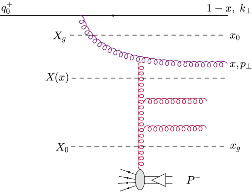
Figure 1: An illustration of the LO high-energy evolution of the ‘cross-section for quark production’ $\mathcal{S}(\bm{k},X_{g})$ (the Fourier transform of the dipole $S$–matrix). The ‘primary gluon’ (the first gluon emission by the quark, which carries a longitudinal momentum fraction $x\ll 1$ is) viewed as a part of the wavefunction of the incoming quark (a right mover). The subsequent emissions are rather associated with the evolution of the gluon distribution in the nuclear target (a left mover), within the range $X(x)<X<X_{0}$, with $X(x)=X_{g}/x$ and $X_{0}\sim 1$. Alternatively, and equivalently at LLA, they can be associated with the evolution of the wavefunction of the primary quark-gluon pair (a right mover) within the ‘plus’ momentum range $x_{g}<x^{\prime}<x$.

Under these assumptions, the second term in the r.h.s. of Eq. (8) (the light-cone energy of the primary gluon) dominates over the first one and, moreover, one can ignore the difference between $p_{\perp}$ and $k_{\perp}$ when computing the evolution variables $Y=\ln(1/X)$ and $y=\ln(1/x)$.

The above argument can be immediately extended to an arbitrary separation of the LO high-energy evolution between the quark projectile and the nuclear target: successive emissions in the projectile are strongly ordered in $x$ but have comparable transverse momenta, hence both energy conservation and the energy denominators are controlled by the last emitted gluon — the one with the smallest value of $x$ and a transverse momentum of order $k_{\perp}$. Accordingly, instead of Eq. (8), one can use the following, simpler, relation,

$$X(x)\,=\,\frac{k_{\perp}^{2}}{x\hat{s}}\,=\,\frac{X_{g}}{x}\,,$$ (9)

(or $Y=Y_{g}-y$) in order to connect the LO evolution of the projectile to that of the target. The differences between (8) and (9) become however important starting with NLO, as we shall see.

The above discussion can be summarized by the following integral representation of the solution to the BK equation, illustrated in Fig. 1, in which the total evolution is explicitly split between exactly one soft gluon ($x\ll 1$) in the quark wavefunction and an arbitrary number of soft gluons ($X\ll 1$) in the wavefunction of the target:

$$S\big{(}\bm{x},\bm{y};X_{g}\big{)}=S_{0}(\bm{x},\bm{y})+\frac{\bar{\alpha}_{s}}{2\pi}\, \int_{x_{g}}^{1}\frac{{\rm d}x}{x}\int{\rm d}^{2}\bm{z}\,\frac{(\bm{x}-\bm{y})^{2}}{(\bm{x}-\bm{z})^{2}(\bm{z}-\bm{y})^{2}}$$

$$\,\Big{[}S\big{(}\bm{x},\bm{z};X(x)\big{)}S\big{(}\bm{z},\bm{y};X(x)\big{)}-S\big{(}\bm{x},\bm{y};X(x)\big{)}\Big{]}\,.$$ (10)

In this equation, $S_{0}$ is the initial condition at $X_{0}\simeq 1$ and the lower limit $x_{g}\equiv k_{\perp}^{2}/\hat{s}$ for the integral over $x$ corresponds via (9) to $X=1$, i.e. to the situation where the soft gluon from the projectile probes bare nucleons from the target. Eq. (2.3) can also be viewed as purely target evolution provided one changes the integration variable from $x$ to $X\equiv X(x)$. Then it becomes obvious that this is the same as Eq. (7) integrated over $Y$, from $Y_{0}=0$ up to $Y_{g}$.

(a)

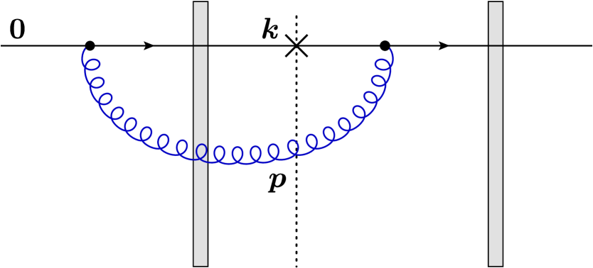
(b)

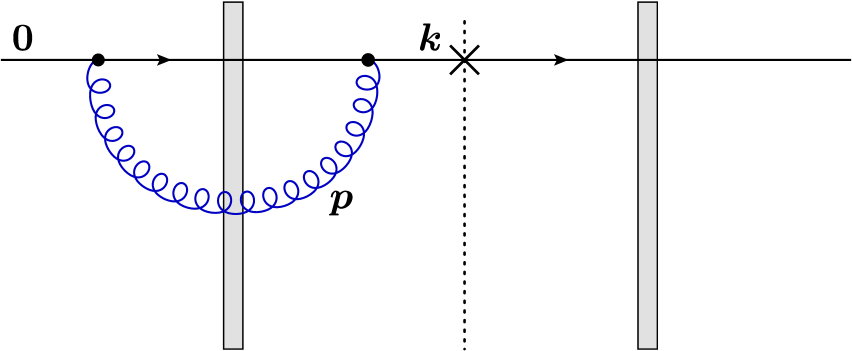
(c)

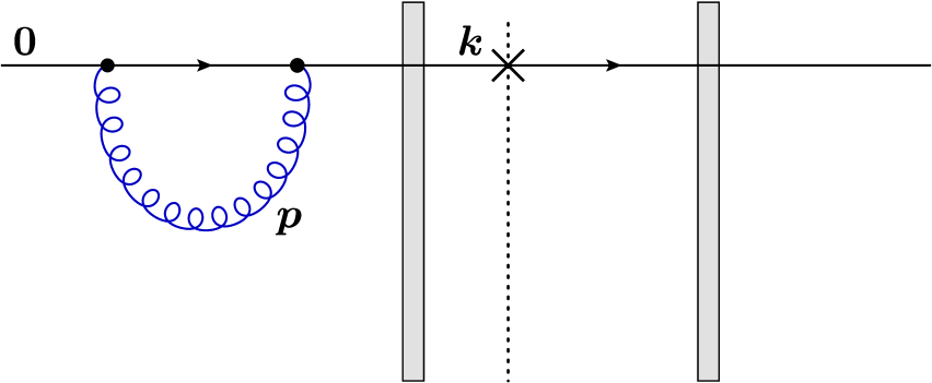
(d)

Figure 2: Typical diagrams contributing to the high-energy evolution of the quark production at leading order. (a) Real diagram, in which all possible interactions of the gluon with the target cancel one another. (b) Real diagram in which the gluon in the CCA is emitted before the collision with the shockwave, while in the DA is emitted after the collision. (c,d) Virtual diagrams in which the gluon interacts, or not, with the shockwave. Only transverse momenta are shown in all the graphs.

In Fig. 2, we present some Feynman graphs which contribute to the integral term in Eq. (2.3). We do not use the dipole picture, rather we show graphs which enter the cross-section for quark production (so, in particular, we use the transverse momentum representation). The nuclear target evolved up to $X(x)$ is represented as a shockwave (recall that we are still in a frame where the target is ultrarelativistic). There are two types of graphs: ‘real’, where the primary gluon appears in the final state — it is emitted in the direct amplitude (DA) and reabsorbed in the complex conjugate amplitude (CCA) — and ‘virtual’, where the gluon is both emitted and reabsorbed on the same side of the cut (either in the DA, or in the CCA). It is instructive to notice how such graphs are generated from the BK equation (2.3): decomposing the dipole kernel there as

$${\mathcal{M}}_{\bm{x}\bm{y}\bm{z}}\equiv\frac{(\bm{x}-\bm{y})^{2}}{(\bm{x}-\bm{z})^{2}(\bm{y}-\bm{z})^{2}}=\frac{1}{(\bm{x}-\bm{z})^{2}}+\frac{1}{(\bm{y}-\bm{z})^{2}}-2\,\frac{x^{i}-z^{i}}{(\bm{x}-\bm{z})^{2}}\frac{y^{i}-z^{i}}{(\bm{y}-\bm{z})^{2}}\,,$$ (11)

one can check that the ‘virtual’ terms are generated by the first 2 terms in the r.h.s. of Eq. (11), whereas the ‘real’ terms come from the third one. Note that, for the particular ‘real’ term where the gluon crosses the shockwave twice, cf. Fig. 2.a, the gluon interactions cancel between the DA and the CCA, by unitarity, hence the respective contribution to the r.h.s. of Eq. (2.3) involves only the scattering of the original quark (as described by the dipole $S$-matrix $S\big{(}\bm{x},\bm{y};X(x)\big{)}$).

Given the ‘boost-invariance’ of the (LO) BK equation alluded to above, one may wonder what can be the utility of dividing the evolution between target and projectile, as we did above. As a matter of facts, there are several advantages for doing that. First, one should keep in mind that the laboratory frame for ‘dilute-dense’ (d+Au or p+Pb) collisions at RHIC and the LHC coincides with the COM frame (at RHIC), or is close to it (at the LHC). Hence the picture of the high-energy evolution which is directly visible in the experiments is that of an evolution shared by the two incoming hadrons. Second, we shall shortly argue that the first gluon emission by the incoming quark (the ‘primary gluon’) plays in fact a special role, at least for relatively large $k_{\perp}\gtrsim Q_{s}$. Because of that, it is preferable (and even compulsory, starting with NLO) to view this gluon as a part of the quark evolution, like in Eq. (2.3). Still beyond LO, it is conceptually simpler to associate the high-energy evolution with the target wavefunction. As we shall see, the complete result for the quark multiplicity to NLO, to be presented in Sect. 3, can be viewed as a natural generalization of Eq. (2.3).

2.4 Hard transverse momentum and di-jet events

In this subsection, we shall discuss the physical picture of forward quark production in the IMF of the projectile, or, more generally, in any ‘mixed’ frame, like that illustrated in Fig. 1, where the quark wavefunction contains at least one soft gluon. We would like to show that, in any such a frame, the tail of the quark distribution at relatively high $k_{\perp}$ comes from the recoil in the emission of the primary gluon (the first gluon emitted by the quark). That is, a forward quark with large transverse momentum $k_{\perp}\gtrsim Q_{s}$ is produced in a di-jet event where the quark is accompanied by a recoil gluon and the two particles propagate back-to-back in the transverse plane. This point is important in that it will affect the NLO calculation of the quark production at relatively high $k_{\perp}$, where the negativity problem in the cross-section has been observed.

At a first sight, the prominence of the di-jet configuration at large $k_{\perp}$ might look rather obvious, as an immediate consequence of transverse momentum conservation at the emission vertex. But the situation is a bit more subtle, since a large transverse momentum can also be transferred by the target, via a sufficiently hard scattering. As a matter of facts, in the classical approximation at low energy (i.e. in the absence of any evolution), a power-like tail $\propto 1/k_{\perp}^{4}$ in the quark distribution at high $k_{\perp}$ is generated via Coulomb scattering (see below). The same physical picture would also hold at high energy (within the limits of the LLA), but only in the target IMF, where there is no gluon emission by the quark. But in a frame where the quark itself is allowed to radiate, the phase-space for high-energy evolution at high $k_{\perp}$ favors configurations where the momentum $\ell_{\perp}$ transferred from the target to the projectile (the quark together with its small-$x$ radiation) is relatively low, $\ell_{\perp}\ll k_{\perp}$. Because of that, the only way to produce a quark with very large $k_{\perp}$ is via a di-jet event, as anticipated.

Consider first the semi-classical approximation (no evolution), that we shall treat within the MV model. Since we are interested in a relatively hard quark with $k_{\perp}\gg Q_{s}$, we can limit ourselves to the single-scattering approximation, as obtained by expanding the Wilson lines in Eq. (5) up to second order in the target color fields $A^{-}$ (see Fig. 3). Writing $S=1-T$, one finds the dipole scattering amplitude in the 2-gluon exchange approximation as (recall that $\bm{r}=\bm{x}-\bm{y}$)

$$T_{0}(\bm{r}) =\frac{g^{2}}{2N_{c}}\left\langle\big{(}A^{-}_{a}(\bm{x})-A^{-}_{a}(\bm{y})\big{)}^{2}\right\rangle$$

$$=g^{2}C_{F}\!\int\frac{{\rm d}^{2}\bm{q}}{(2\pi)^{2}}\frac{\mu^{2}}{q_{\perp}^{4}}\big{[}1-{\rm e}^{i\bm{q}\cdot\bm{r}}\big{]}\simeq\frac{\alpha_{s}C_{F}}{4}\,r^{2}\mu^{2}\ln\frac{1}{r^{2}\Lambda^{2}}\,,$$ (12)

where in the second line we have used the MV model expression for the 2-point correlator of the color fields in a dense nucleus (with atomic number $A$ and transverse area $\pi R_{A}^{2}$), namely

$$\int{\rm d}x^{+}{\rm d}y^{+}\left\langle A^{-}_{a}(x^{+},\bm{q})\,A^{-}_{b}(y^{+},\bm{\ell})\right\rangle_{{\rm\scriptscriptstyle MV}}=(2\pi)^{2}\delta^{(2)}(\bm{q}+\bm{\ell})\delta_{ab}\,\frac{\mu^{2}}{\bm{q}^{4}}\,,\qquad\mu^{2}=\frac{g^{2}C_{F}AN_{c}}{(N_{c}^{2}-1)\pi R_{A}^{2}}\,.$$ (13)

The quantity $\mu^{2}$ represents the color charge squared of the $AN_{c}$ valence quarks (treated as uncorrelated color sources) per unit transverse area. The variable $\bm{q}$ that is integrated over in Eq. (2.4) is the transverse momentum transferred from the target to the dipole and $\Lambda$ is an infrared cutoff (say, the confinement scale). The unit term within the square brackets corresponds to the case where the two exchanged gluons are attached to a same quark leg within the dipole, while the exponential ${\rm e}^{i\bm{q}\cdot\bm{r}}$ refers to attachments to both legs (see Fig. 3). For relatively small dipole sizes $r\ll 1/\Lambda$, the integral over $q_{\perp}$ develops a transverse logarithm which can be isolated by expanding out the exponential to second order. This yields the final result shown in Eq. (2.4). When this result becomes of $\mathcal{O}{(1)}$, multiple scattering becomes important and the above approximation breaks down. This condition defines the target saturation momentum $Q_{0}$ at low energy: $T_{0}(r)\sim 1$ for $r\simeq 1/Q_{0}$.

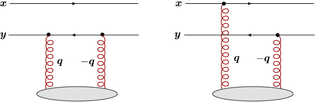
Figure 3: Diagrams for the elastic scattering of the dipole in the single scattering approximation, or 2 gluon exchange. The blob at the bottom of the diagram refers to the average over the color fields in the target, which effectively generates the gluon distribution on the resolution scale $r$ of the dipole projectile.

This simple calculation makes it clear that the scattering of a small dipole ($1/r\gg Q_{0}$) is controlled by relatively soft gluon exchanges ($\Lambda\ll q_{\perp}\ll 1/r$) with the target. Let us similarly compute the quark production, for a quark with large transverse momentum $k_{\perp}\gg Q_{0}$. When taking the Fourier transform of $T_{0}(\bm{r})$, the unit term within the square brackets in Eq. (2.4) does not matter (this would describe an elastic scattering without net momentum transfer; see Fig. 4), whereas the exponential term there selects $\bm{q}=\bm{k}$. This is simply the expression of momentum conservation and confirms that one needs a hard (inelastic) scattering in order to produce a hight-$k_{\perp}$ quark. One thus finds $\mathcal{T}_{0}(k_{\perp})=g^{2}C_{F}\mu^{2}/k_{\perp}^{4}$, which is recognized as the Rutherford cross-section for the Coulomb scattering between the quark and the nucleus; therefore,

$$\frac{{\rm d}N^{pA\to qX}}{{\rm d}^{2}\bm{k}\,{\rm d}\eta}\bigg{|}_{{\rm\scriptscriptstyle MV}}\simeq\,x_{p}q(x_{p})\,\frac{\alpha_{s}C_{F}\mu^{2}}{\pi k_{\perp}^{4}}\,\qquad\mbox{for}\quad k_{\perp}\gg Q_{0}\,.$$ (14)

We shall now study the high-energy evolution of the above results, in the double logarithmic approximation (DLA) which is appropriate for sufficiently small dipole sizes, or large $k_{\perp}$. For the present purposes, it is convenient to work in a frame where this is viewed as projectile evolution; that is, the soft gluons belong to the wavefunction of the quark and they are all right movers.

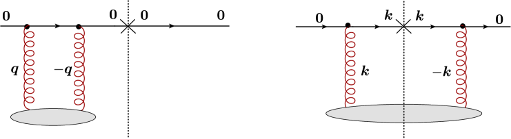
Figure 4: Diagrams for quark production in the 2-gluon exchange approximation. The diagram on the left describes an elastic scattering in the DA and no scattering in the CCA; hence it contributes to quark production only for $\bm{k}=0$. The diagram on the right describes an inelastic scattering in the DA and another one in the CCA. The final momentum $\bm{k}$ of the produced quark is transferred by the target. Momenta are flowing from left to right both in the DA and in the CCA and from bottom to top in the exchange (red) gluons.

In transverse coordinate space, the DLA corresponds to the splitting of the original dipole $(\bm{x},\,\bm{y})$ into two daughter dipoles, $(\bm{x},\,\bm{z})$ and $(\bm{z},\,\bm{y})$, whose transverse sizes are much larger, but still small enough to undergo only single scattering: $r\ll\bar{z}\ll 1/Q_{0}$, with $\bar{z}\equiv|\bm{x}-\bm{z}|\simeq|\bm{z}-\bm{y}|$. The respective evolution equation is obtained from the general BK equation (7) by (i) linearizing w.r.t. $T=1-S$ (by itself, this step yields the BFKL equation), then (ii) approximating the dipole kernel as ${\mathcal{M}}_{\bm{x}\bm{y}\bm{z}}\simeq r^{2}/\bar{z}^{4}$, and (iii) keeping only the scattering amplitudes $T(\bm{x},\bm{z})+T(\bm{z},\bm{y})\simeq 2T(\bar{z})$ for the two daughter dipoles, whose scattering is stronger (since $T(r)\propto r^{2}$ in this physical regime). One thus finds (as before, we use $y=\ln(1/x)$ for the evolution ‘time’ of the projectile)

$$\frac{\partial}{\partial y}\,T(r,y)={\bar{\alpha}_{s}}\,r^{2}\int_{r^{2}}^{1/Q_{0}^{2}}\frac{{\rm d}\bar{z}^{2}}{\bar{z}^{4}}\,T(\bar{z},y)\,.$$ (15)

Since $T(\bar{z})\propto\bar{z}^{2}$, the integral in the r.h.s. is clearly logarithmic. The first iteration of this equation, as obtained by evaluating its r.h.s. with the amplitude $T_{0}$ from Eq. (2.4), describes the first gluon emission by the parent dipole. The physical picture of this emission follows from the previous discussion: the original dipole with size $r$ emits a relatively soft gluon with transverse momentum $p_{\perp}\sim 1/\bar{z}$ within the range $Q_{0}\ll p_{\perp}\ll 1/r$, which then suffers an even softer scattering off the nuclear target, with transferred momentum $\Lambda\lesssim q_{\perp}\ll p_{\perp}$ (see Fig. 5 left). This picture extends to the whole gluon cascade generated by iterating Eq. (15): successive gluon emissions are strongly ordered not only in $x$ but also in transverse momenta, and the final exchange with the target is even softer.

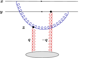
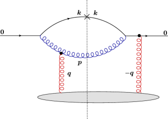
Figure 5: Left: one step in the DLA evolution of a small dipole, with size $r\ll 1/Q_{s}$. The daughter gluon is typical soft and thus emitted at a large distance $|\bm{z}-\bm{x}|\simeq|\bm{z}-\bm{y}|\gg r$ from the parent dipole. The gluon exchange $\bm{q}$ with the nuclear target is even softer. Right: one step in the DLA evolution of the cross-section for quark production, at large transverse momentum $k_{\perp}\gg Q_{s}$. The primary gluon is as hard as the produced quark and they are both much harder than the gluon exchanged with the target: $k_{\perp}\simeq p_{\perp}\gg q_{\perp}=|\bm{k}+\bm{p}|$. The other diagrams contributing to this process at the level of the amplitude are shown in Fig. 6.

We now turn to the corresponding picture in transverse momentum space, that is, to the problem of quark production (see Fig. 5 right and also Fig. 6). The momentum-space DLA equation reads

$$\frac{\partial}{\partial y}\,\mathcal{T}(k_{\perp},y)=\frac{\bar{\alpha}_{s}}{k_{\perp}^{4}}\int_{Q_{0}^{2}}^{k_{\perp}^{2}}{\rm d}q_{\perp}^{2}\,q_{\perp}^{2}\mathcal{T}(q_{\perp},y)\,,$$ (16)

where the integral in the r.h.s. is indeed logarithmic, since $\mathcal{T}(q_{\perp},y)\propto 1/q_{\perp}^{4}$. Within this integral, $\mathcal{T}(q_{\perp},y)$ should be interpreted as the cross-section for a single scattering, with transferred momentum $q_{\perp}$, between partons in the quark wavefunction and the target. The factor ${\bar{\alpha}_{s}}/{k_{\perp}^{4}}$ in front of the integral does not represent anymore a $t$-channel exchange with the target, as in Eq. (14), but rather it comes from the propagator of the intermediate quark, or gluon, in the $s$-channel (see Fig. 6). Hence, the physical picture of the first emission is now as follows: the original quark with zero transverse momentum emits a gluon with momentum $\bm{p}$ and turns into a final quark with momentum $\bm{k}$, while at the same time receiving a momentum transfer $\bm{q}$ from the target (via a scattering that can occur either before, or after the splitting). Transverse momentum conservation requires $\bm{q}=\bm{k}+\bm{p}$. But the overall cross-section, as described by Eq. (16), favors soft scattering, with transferred momenta $q_{\perp}\ll k_{\perp}$. Accordingly, the first emitted gluon must be hard, $p_{\perp}\simeq k_{\perp}$, to balance the momentum of the produced quark.

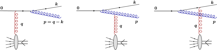
Figure 6: The 3 diagrams which contribute to the production of a quark-gluon pair in the final state in the regime where both the quark and the gluon are relatively hard ($k_{\perp}\simeq p_{\perp}\gg q_{\perp}=|\bm{k}+\bm{p}|$).

As for the subsequent gluon emissions, starting with the second one, they follow the standard DLA ordering, in both $x$ and $p_{\perp}$, as in the respective calculation in coordinate space, cf. Eq. (15). This argument too shows that, when computing particle production, it is quite natural to associate the primary gluon with the wavefunction of the produced particle, whereas the other gluons are more conveniently included in the gluon distribution of the target, as measured by the hard splitting process. While natural already at LLA, this viewpoint becomes almost unavoidable when moving to the next-to-leading order calculation, where the primary gluon is also allowed to have a large longitudinal momentum $p^{+}\sim q^{+}_{0}$. The NLO calculation will be discussed in the next section.

3 Next-to-leading order

In order to move on to next-to-leading order (NLO) accuracy, one must relax some of the previous approximations and add new contributions which start at NLO. By inspection of the LO result (3), it is clear that one ingredient required in that sense is the NLO version of the B-JIMWLK (or BK) equations Balitsky:2008zza ; Balitsky:2013fea ; Kovner:2013ona , together with their all-order ‘collinear’ resummations Beuf:2014uia ; Iancu:2015vea ; Iancu:2015joa ; Hatta:2016ujq . This in particular means that some gluon emissions must be computed beyond the eikonal approximation: besides the effect of order $\alpha_{s}Y$, which dominates at high energy, one must also keep, for each such an emission, the ‘pure-$\alpha_{s}$’ corrections which are not enhanced by the rapidity logarithm $Y$ (but may be accompanied by transverse logarithms). So long as these NLO corrections refer to generic gluons inside the cascade, they can be absorbed into a renormalization of the kernel of the evolution equation. The same is true for the quark-antiquark loop which at NLO can be inserted within any of the gluon lines. But the NLO corrections associated with the ‘primary gluon’ (the very first emission by the leading quark) must rather be used to renormalize the ‘impact factor’, i.e. the value of the cross-section in the absence of high-energy evolution.

At LO, the impact factor is the cross-section for the inelastic scattering between the leading quark and the low energy nucleus (say, as described by the MV model). Equivalently (to the accuracy of interest), it can be written as the $S$–matrix for the elastic scattering of a $q\bar{q}$ dipole. At NLO, one must add the impact factor encoding the inelastic scattering of the quark-gluon pair made with the leading quark and the primary gluon. Unlike the emission of the primary gluon, which must be computed exactly, the scattering between the quark-gluon pair and the target can still be computed in the eikonal approximation and thus related to elastic scattering amplitudes for color multipoles Marquet:2007vb ; Dominguez:2011wm ; Chirilli:2012jd .

So, it may look like, in order to compute quark production at NLO, one must dress the two contributions to the impact factor aforementioned with the high-energy evolutions of the respective scattering amplitudes (themselves computed at NLO) and then add the results. But a moment of thinking reveals that the two pieces of the impact factor mix with each other under the high-energy evolution: a part of the primary gluon emission that we have explicitly included in the NLO impact factor is also included (within the limits of the eikonal approximation) as the first small-$x$ gluon in the evolution of the dipole $S$–matrix from the LO cross-section (3). This is the problem of over-counting. Previous papers in the literature Chirilli:2011km ; Chirilli:2012jd proposed a solution to this problem, in the form of a ‘plus’ prescription which subtracts the LO evolution from the NLO impact factor. This prescription however appears to be responsible for the problem with the negativity of the cross-section discussed in the Introduction.

In what follows, we shall propose a different way to organize the calculation, which avoids the over-counting without performing any subtraction. Our strategy will naturally exploit the structure of perturbation theory at high energy. As we shall see, the contribution to the cross-section which includes the NLO correction to the impact factor does also encode, completely and faithfully, the LO evolution of the dipole $S$-matrix. Hence, by computing this contribution as it stands, one can simultaneously include both effects without any ambiguity, or over-counting. On top of that, there is a NLO correction to the evolution of the color dipole; this will be clearly identified and related to recent results concerning the NLO version of the BK equation Balitsky:2008zza and its collinear resummations Iancu:2015vea ; Iancu:2015joa .

3.1 Revisiting the NLO calculation by Chirilli, Xiao, and Yuan

In this subsection, we shall exhibit, discuss, and adapt to our present purposes the result of the NLO calculation of the impact factor by Chirilli, Xiao, and Yuan Chirilli:2011km ; Chirilli:2012jd . First, we shall display their ‘bare’, or ‘unsubtracted’, result, where the soft divergence at $x\to 0$ is explicit. Then we shall briefly mention the ‘plus’ prescription advocated in Refs. Chirilli:2011km ; Chirilli:2012jd in order to subtract the rapidity divergence. (We shall return to this point in Sect. 3.5.) Finally, we shall explain our strategy to deal with this problem, which is to use kinematical constraints like energy conservation in order to cut off the soft divergence and at the same time fix the rapidity variables for the evolution of the dipole $S$-matrices. The only subtle point here is the treatment of the virtual corrections, where the phase-space for the emission of the primary gluon is not directly constrained by the kinematics. Yet, as we shall demonstrate via explicit calculations (in Appendix A), the same lower limit on $x$ applies in that case too, albeit its emergence is now dynamical.

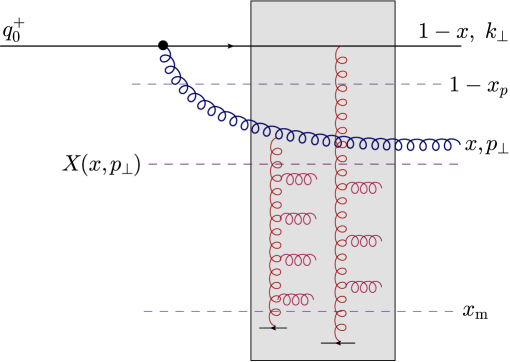
Figure 7: Pictorial representation of a typical amplitude contributing to the NLO piece of the impact factor. This is a ‘real’ amplitude, in the sense that the primary gluon is released in the final state.

The NLO result in Refs. Chirilli:2011km ; Chirilli:2012jd has been obtained by evaluating Feynman graphs like that illustrated in Fig. 7 in which the emission of the primary gluon is treated exactly. There is a similar graph where the gluon emission occurs after the scattering between the quark and the target. And there are of course virtual graphs, whose evaluation is somewhat subtle as just mentioned and that we shall deal with in some detail. (See Figs. 8 and 9 below for more examples of Feynman graphs.) After the scattering, both the quark and the gluon will fragment into hadrons and thus contribute to single-inclusive hadron production. There is also another channel where the original collinear parton is a gluon, which splits into a pair of gluons, or into a quark-antiquark pair, in the process of scattering. As before, we shall omit the discussion of the fragmentation process and concentrate on quark production alone (see Refs. Chirilli:2011km ; Chirilli:2012jd for a complete discussion and also Altinoluk:2014eka for an alternative calculation, whose precise relation to the original results in Chirilli:2011km ; Chirilli:2012jd is still unclear). That is, the primary gluon is not measured, so one needs to integrate out its kinematics — the longitudinal momentum fraction $x=p^{+}/q_{0}^{+}$ and the transverse momentum $\bm{p}$.

The NLO result in Refs. Chirilli:2011km ; Chirilli:2012jd can be conveniently written as the sum of 2 pieces:

(A) A piece proportional to the quark Casimir $C_{\rm F}$ which develops no logarithm at small $x$ (the respective integrand vanishes as $x\to 0$), but has collinear divergences in the transverse momentum integrations. In Chirilli:2011km ; Chirilli:2012jd , these divergences have been isolated with the help of dimensional regularization and reabsorbed into the leading-order DGLAP evolution of the quark distribution function $q(x_{p})$ (if the primary emission occurs prior to scattering) and of the quark-to-hadrons fragmentation function (if the emission occurs after the scattering). This prescription leaves a finite remainder of NLO order whose explicit evaluation poses no special problem.

(B) A piece proportional to the gluon Casimir $N_{\rm c}$ which is free of collinear problems but develops a logarithm at small $x$ (the respective integral over $x$ exhibits a logarithmic divergence at $x\to 0$ in the absence of any physical regulator). The proper way to deal with this ‘rapidity divergence’ at small $x$ represents our main concern in this paper. To better focus on this problem while avoiding cumbersome notations, we shall omit the piece proportional to $C_{\rm F}$ in what follows. (This piece can be easily added to our main result shown in Eq. (3.2) below.) As for the second piece, proportional to $N_{\rm c}$, we start by displaying the original result, as presented in Refs. Chirilli:2011km ; Chirilli:2012jd :

$$\frac{{\rm d}N^{pA\to qX}}{{\rm d}^{2}\bm{k}\,{\rm d}\eta}\bigg{|}_{{\rm\scriptscriptstyle NLO}}^{\rm unsub}=\frac{\alpha_{s}N_{\rm c}}{(2\pi)^{2}}\int_{0}^{1}{\rm d}\xi\,\frac{1+\xi^{2}}{1-\xi}\left\{\frac{x_{p}}{\xi}q\left(\frac{x_{p}}{\xi}\right)\mathcal{J}(\bm{k},\xi)-x_{p}q\left(x_{p}\right)\mathcal{J}_{v}(\bm{k},\xi)\right\},$$ (17)

where $\xi\equiv 1-x$ and the two functions $\mathcal{J}(\bm{k},\xi)$ and $\mathcal{J}_{v}(\bm{k},\xi)$ correspond to real and virtual contributions to the process illustrated in Fig. 7. They read (our present notations are slightly different from the original ones Refs. Chirilli:2011km ; Chirilli:2012jd , but follow closely the recent paper Ducloue:2016shw )

$$\mathcal{J}(\bm{k},\xi)=\!\int\frac{{\rm d}^{2}\bm{q}}{(2\pi)^{2}}\frac{2(\bm{k}-\xi\bm{q})\cdot(\bm{k}-\bm{q})}{(\bm{k}-\xi\bm{q})^{2}(\bm{k}-\bm{q})^{2}}\mathcal{S}(\bm{q})-\int\!\frac{{\rm d}^{2}\bm{q}}{(2\pi)^{2}}\frac{{\rm d}^{2}\bm{\ell}}{(2\pi)^{2}}\frac{2(\bm{k}-\xi\bm{q})\cdot(\bm{k}-\bm{\ell})}{(\bm{k}-\xi\bm{q})^{2}(\bm{k}-\bm{\ell})^{2}}\mathcal{S}(\bm{q})\mathcal{S}(\bm{\ell}),$$ (18)

and respectively

$$\mathcal{J}_{v}(\bm{k},\xi)=\mathcal{S}(\bm{k})\left[\int\!\frac{{\rm d}^{2}\bm{q}}{(2\pi)^{2}}\frac{2(\xi\bm{k}-\bm{q})\cdot(\bm{k}-\bm{q})}{(\xi\bm{k}-\bm{q})^{2}(\bm{k}-\bm{q})^{2}}-\int\!\frac{{\rm d}^{2}\bm{q}}{(2\pi)^{2}}\frac{{\rm d}^{2}\bm{\ell}}{(2\pi)^{2}}\frac{2(\xi\bm{k}-\bm{q})\cdot(\bm{\ell}-\bm{q})}{(\xi\bm{k}-\bm{q})^{2}(\bm{\ell}-\bm{q})^{2}}\mathcal{S}(\bm{\ell})\right].$$ (19)

As before, the dipole $S$-matrices like $\mathcal{S}(\bm{k})$ or $\mathcal{S}(\bm{q})$ refer to dipoles in the fundamental representation (cf. footnote 9). To simplify writing, we have considered the large $N_{\rm c}$ limit, in which the scattering of a system of two dipoles factorizes as the product of two individual dipole $S$-matrices, but this limit is not essential for what follows.

The variables $\bm{q}$ and $\bm{\ell}$ which appear in the above integrations represent transverse momenta exchanged between the target and the quark-gluon pair. For what follows, it is important to understand their precise meaning and notably their relation with the transverse momentum $\bm{p}$ taken by the primary gluon. By following the derivation of these results in Refs. Chirilli:2011km ; Chirilli:2012jd , one can check that $\bm{q}=\bm{p}+\bm{k}$ whereas $\bm{\ell}$ is independent of $\bm{p}$. For more clarity, let us briefly discuss the physical interpretation of the various terms in Eqs. (18) and (19).

The ‘real’ terms in Eq. (18) represent processes where the primary gluon, albeit not measured, is released in the final state (see Fig. 8). For such processes, longitudinal momentum conservation implies $\xi=k^{+}/q^{+}_{0}$. The first term in Eq. (18), which is linear in $\mathcal{S}(\bm{q})$, represents situations where the hard splitting occurs either after the collision, or prior to it, in both the DA and the CCA. In these cases, the gluon either does not interact with the target at all (emissions after the collision), or the effects of its interaction cancel out from the final result, by unitarity, because the gluon is not measured (emissions before the collision). Accordingly, there is only one dipole $S$-matrix, $\mathcal{S}(\bm{q})$, which physically describes the inelastic scattering of the quark. This scattering transfers a non-zero transverse momentum $\bm{q}$ to the quark; then momentum conservation implies $\bm{q}=\bm{p}+\bm{k}$, as aforementioned.

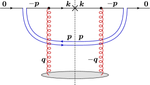
(a)

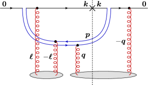
(b)

Figure 8: Production of a quark with a transverse momentum $\bm{k}$. Typical real diagrams, i.e. diagrams in which the gluon is crossing the cut, but at the same time is integrated (cf. Eq. (18)). The primary gluon is represented as a $q\bar{q}$ pair, as appropriate at large $N_{c}$. (a) Left: Diagram contributing to the real term proportional to $\mathcal{S}(\bm{q})$ and which originates from $S(\bm{x},\bm{y})$ in coordinate space. All possible interactions of the gluon with the target cancel each other. (b) Right: Diagram contributing to the real term proportional to $\mathcal{S}(\bm{q})\mathcal{S}(\bm{\ell})$ and which originates from $S(\bm{x},\bm{z})S(\bm{z},\bm{y})$ in coordinate space. In both diagrams the target transfers momentum $\bm{q}=\bm{p}+\bm{k}$ to the final state. Momenta are flowing from left to right both in the DA and in the CCA and from bottom to top in the exchange (red) gluons.

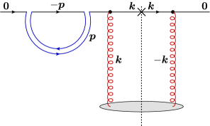
(a)

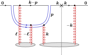
(b)

Figure 9: Production of a quark with a transverse momentum $\bm{k}$. Typical virtual diagrams, i.e. diagrams in which the gluon is not crossing the cut (cf. Eq. (19)). (a) Left: Diagram contributing to the virtual term proportional to $\mathcal{S}(\bm{k})$, which originates from $S(\bm{x},\bm{y})$ in coordinate space (b) Right: Diagram contributing to the real term proportional to $\mathcal{S}(\bm{k})\mathcal{S}(\bm{\ell})$ and which originates from $S(\bm{x},\bm{z})S(\bm{z},\bm{y})$ in coordinate space. Momenta are flowing from left to right both in the DA and in the CCA and from bottom to top in the exchange (red) gluons.

The second term in Eq. (18), bilinear in the dipole $S$-matrix, corresponds to interference processes, where the primary gluon is emitted prior to scattering in the direct amplitude (DA) and after the scattering in the complex conjugate amplitude (CCA), or vice-versa. In such processes, both the quark and the gluon can participate in the collision. At large $N_{c}$, this yields 2 dipole $S$-matrices: one made with the quark in the DA and the antiquark piece of the gluon, the other one with the quark piece of the gluon and the antiquark in CCA. One of these $S$-matrices, denoted as $\mathcal{S}(\bm{\ell})$ in (18), describes the elastic scattering of a physical dipole — i.e. a dipole whose both fermion legs exist on the same side of the cut (either in the DA, or in the CCA). For this elastic scattering, there is no net transfer of transverse momentum; e.g., if $\mathcal{S}(\bm{\ell})$ is computed in the 2-gluon exchange approximation, then the momentum $\bm{\ell}$ transferred by the first exchanged gluon towards the dipole is subsequently taken back by the second exchanged gluon. The other dipole $S$-matrix, $\mathcal{S}(\bm{q})$, describes an inelastic scattering with net momentum transfer $\bm{q}=\bm{p}+\bm{k}$.

Consider similarly the ‘virtual’ contributions encoded in (19) (see Fig. 9). In that case, the primary gluon is both emitted and reabsorbed on the same side of the cut, hence the momentum $\bm{k}$ of the produced quark fully comes via inelastic scattering (and $k^{+}=q_{0}^{+}$). In the first term in (19), the gluon fluctuation has no overlap with the target, hence the (inelastic) scattering refers to the quark alone. In the second term, the gluon can scatter too. Accordingly, this term involve 2 dipole $S$-matrices, one describing an elastic scattering ($\mathcal{S}(\bm{\ell})$), the other one an inelastic one ($\mathcal{S}(\bm{k})$).

The following observations will be useful for the subsequent arguments:

(i) In Eq. (17) one recognizes the full LO DGLAP quark-to-quark splitting function $P_{qq}(\xi)$, in line with the fact that the gluon emission has been treated exactly, and not in the eikonal approximation.

(ii) In Eqs. (18) and (19), the splitting fraction $\xi$ is visible only in the various kernels describing the transverse momentum structure of the hard splitting, which in turn have been generated by combining the light-cone energy denominator with factors coming from the splitting vertex.

(iii) The various dipole $S$-matrices in Eqs. (18) and (19) are supposed to describe scattering off the nuclear gluon distribution evolved up to the right ‘rapidity’ ($Y=\ln(1/X)$) scale, but this scale is left unspecified in the above equations. For the ‘real’ contributions at least, we know by now what is the typical longitudinal momentum fraction $X$ of the gluons from the target which are probed by this scattering: this is the value $X(x,p_{\perp})$ given by Eq. (8). Hence, the dipole $S$-matrices in Eq. (18) must be evaluated at $X\simeq X(x,p_{\perp})$, where it is understood that $\bm{p}=\bm{q}-\bm{k}$. We shall later demonstrate that $X(x,p_{\perp})$ with $\bm{p}=\bm{q}-\bm{k}$ is also the appropriate choice for the rapidity argument of $S$-matrices which enter the ‘virtual’ terms in Eq. (19). This means that, strictly speaking, one cannot factorize the $S$-matrix $\mathcal{S}(\bm{k})$ in front of the integrals in Eq. (19), in contrast to the results in Chirilli:2011km ; Chirilli:2012jd .

(iv) The integral over $\xi$ in Eq. (17) seems to develop a logarithmic singularity at $\xi=1$, meaning an infrared divergence associated with the emission of very soft ($x\to 0$) gluons. (This is the meaning of the upper label ‘unsub’ in the l.h.s. of Eq. (17).) As already mentioned, Refs. Chirilli:2011km ; Chirilli:2012jd proposed to eliminate this divergence via the ‘plus’ prescription, defined as (for a generic function $F(\xi)$)

$$\int_{0}^{1}{\rm d}\xi\,\frac{F(\xi)}{1-\xi}\,\longrightarrow\,\int_{0}^{1}{\rm d}\xi\,\frac{F(\xi)}{(1-\xi)_{+}}\,\equiv\,\int_{0}^{1}{\rm d}\xi\,\frac{F(\xi)-F(1)}{1-\xi}\,.$$ (20)

After this subtraction, the result in Eqs. (17)– (19) is supposed to represent a purely NLO correction, to be added to the respective LO result in Eq. (3). We shall further discuss this particular prescription in Sect. 3.5, but already at this level it should be clear that, as a matter of facts, there is no physical singularity in Eq. (17): for the ‘real’ terms at least, the integral over $\xi$ is cut off near $\xi=1$ by energy conservation, cf. Eq. (8). Specifically, by using Eq. (8) together with the kinematical limit $X(x,p_{\perp})\leq 1$, one finds the following lower limit on $x=1-\xi$:

$$x\,\gtrsim\,x_{\rm m}(p_{\perp})\equiv\,\frac{p_{\perp}^{2}}{\hat{s}}\,,$$ (21)

where we also used $x_{\rm m}\ll 1$. Still for the ‘real’ terms, there is also an upper limit $x\leq 1-x_{p}$, coming from the condition $x_{p}/(1-x)\leq 1$ on the longitudinal fraction of the incoming quark.

This lower limit $x\gtrsim x_{\rm m}$, can be recognized as the condition that the lifetime $\Delta x^{+}\sim 2p^{+}/p_{\perp}^{2}$ of the softest primary gluon emission be at least as large as the longitudinal width $1/P^{-}$ of the target (a necessary condition for having significant scattering). This condition has been previously emphasized in Altinoluk:2014eka (the ‘Ioffe time’) and numerically implemented in Watanabe:2015tja (where however the dependence of the various $S$-matrices upon the target rapidity $X(x,p_{\perp})$ has not been taken into account).

The existence of a physical lower limit on $x$ is indeed crucial for our subsequent construction, which will not involve the ‘plus’ prescription, or any other infrared regularization of the integral over $x$. It is therefore important to demonstrate that such a limit exists also for the ‘virtual’ terms in Eq. (19), for which the previous argument on energy conservation does not apply. We shall do that in Appendix A, where we demonstrate that the same lower limit $x\gtrsim x_{\rm m}$ holds also for the ‘virtual’ terms, as a consequence of fine cancellations among the virtual gluon graphs which occur in the complementary region at $x<x_{\rm m}$. Whereas mathematically subtle, the occurrence of such cancellations has a clear physical interpretation: gluon fluctuations with $x<x_{\rm m}$ cannot interact with the target, since their lifetime is too short. Accordingly the emissions of such short-lived gluons cannot modify the $S$-matrix of the projectile. Since ‘real’ emissions with $x<x_{\rm m}$ are anyway forbidden by energy conservation, it follows that the respective ‘virtual’ graphs must cancel among themselves. The precise way how such cancellations occur is demonstrated in Appendix A (for the somewhat simpler, but general enough, situation where the target itself is a quark).

(v) If one takes the limit $\xi\to 1$ (i.e. $x\to 0$) in the transverse kernels in Eqs. (18) and (19) (but not necessarily also in their implicit dependence upon $x$ via the rapidity cutoff $X(x,p_{\perp})$), then the combination of these two terms which enters Eq. (17) with $\xi\to 1$ reduces to the Fourier transform of the r.h.s. of the BK equation Eq. (7). Specifically,

$$2\pi\bar{\alpha}_{s}\big{[}\mathcal{J}(\bm{k},1)-\mathcal{J}_{v}(\bm{k},1)\big{]}=\int{\rm d}^{2}\bm{r}\,{\rm e}^{-{\rm i}\bm{k}\cdot\bm{r}}\,\frac{\partial}{\partial Y}\,S(\bm{r};Y)$$ (22)

where the notation $\partial S(\bm{r};Y)/\partial Y$ is merely a shortcut for the r.h.s. of (7) with $\bm{r}=\bm{x}-\bm{y}$. The appearance of the BK equation was in fact to be expected: when $\xi\to 1$, Eqs. (17)–(19) describe the emission of a soft primary gluon by the incoming quark, in the eikonal approximation. By definition, the effect of this soft emission on the quark multiplicity is equivalent to the first step in the BK evolution of the respective LO result in Eq. (3). Note however that in general the $S$-matrices implicit in the r.h.s. of Eq. (22) are meant to be computed beyond the LLA and their rapidity argument $X(x,p_{\perp})$ is a complicated function of the kinematics of the emitted gluon.

3.2 CGC factorization at NLO

After this preparation, we are now in a position to present our master formula for the single-inclusive quark multiplicity valid through next-to-leading order (i.e. which includes both the LO and the NLO contributions). The relation between this formula and the factorization scheme proposed in Refs. Chirilli:2011km ; Chirilli:2012jd will be discussed later, in Sect. 3.5. As already mentioned, we systematically omit the NLO corrections proportional to the quark Casimir $C_{\rm F}$, which play no special role for the high-energy evolution. These corrections can be taken over from Refs. Chirilli:2011km ; Chirilli:2012jd and simply added to our master formula, which reads

$$\frac{{\rm d}N^{pA\to qX}}{{\rm d}^{2}\bm{k}\,{\rm d}\eta}\bigg{|}_{{\rm\scriptscriptstyle LO}+{\rm\scriptscriptstyle NLO}}\! =\frac{x_{p}q(x_{p})}{(2\pi)^{2}}\Big{[}{\mathcal{S}}_{0}(\bm{k})+\Delta{\mathcal{S}}(\bm{k},X_{g})\Big{]}+\int\!\frac{{\rm d}^{2}\bm{p}}{(2\pi)^{2}}\int_{x_{\rm m}(p_{\perp})}^{1}\!{\rm d}x\ \frac{\bar{\alpha}_{s}}{2\pi}\,\frac{1+(1-x)^{2}}{2x}$$

$$\times\left\{\frac{x_{p}}{1-x}q\left(\frac{x_{p}}{1-x}\right)\tilde{\mathcal{J}}\big{(}\bm{k},x;\bm{p},X(x,p_{\perp})\big{)}-x_{p}q\left(x_{p}\right)\tilde{\mathcal{J}}_{v}\big{(}\bm{k},x;\bm{p},X(x,p_{\perp})\big{)}\right\}.$$ (23)

This formula is illustrated in Fig. 10. As before, ${\mathcal{S}}_{0}(\bm{k})$ denotes the tree-level contribution to the dipole $S$-matrix, say as given by the MV model (see e.g. Iancu:2002xk ; Iancu:2003xm ; Gelis:2010nm ; Kovchegov:2012mbw for an explicit expression). The quantity $\Delta{\mathcal{S}}(\bm{k},X_{g})$ within the square brackets denotes a NLO correction to the dipole $S$-matrix, to be specified in Sect. 3.4. The last term in Eq. (3.2), which involves a double integration — over the longitudinal fraction $x=1-\xi$ and the transverse momentum $\bm{p}$ of the primary gluon — is the main term for our present purposes. It encodes the impact factor to NLO accuracy, the LO evolution of the dipole $S$-matrix and also a part of the respective NLO contribution (namely, the part which is not included in $\Delta{\mathcal{S}}(\bm{k},X_{g})$; see Sect. 3.4 for details).

The new functions $\tilde{\mathcal{J}}\big{(}\bm{k},x;\bm{p},X(x,p_{\perp})\big{)}$ and $\tilde{\mathcal{J}}_{v}\big{(}\bm{k},x;\bm{p},X(x,p_{\perp})\big{)}$ are essentially the integrands in Eqs. (18) and respectively (19), in which we replaced $\xi\to 1-x$ and $\bm{q}\to\bm{p}+\bm{k}$. (As compared to (18) and (19), we now use $\bm{p}$ and $\bm{\ell}$ as integration variables; the integral over $\bm{p}$ is explicit in Eq. (3.2), while that over $\bm{\ell}$ is included in the definitions of $\tilde{\mathcal{J}}$ and $\tilde{\mathcal{J}}_{v}$.) The notation emphasizes that the various dipole $S$-matrices implicit in these functions should be evaluated at a target rapidity $Y=\ln(1/X)$ with $X=X(x,p_{\perp})$, cf. Eq. (8). The lower limit $x_{\rm m}(p_{\perp})$ is shown in Eq. (21). In the real term, it is understood that the support of the quark distribution limits the integration to $x<1-x_{p}$.

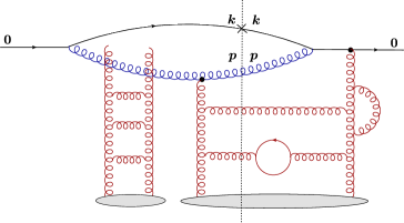
Figure 10: Graphical illustration of the factorization in Eq. (3.2). Left: a diagram describing multiple scattering in the MV model; this is representative for the tree-level term $\mathcal{S}_{0}$ in Eq. (3.2). Right: a diagram which exhibits the primary quark-gluon pair (the NLO impact factor) and its multiple scattering off the gluon distribution of the target, itself evolved to NLO; this is representative for the second term in Eq. (3.2), which encodes all the radiative corrections to the quark multiplicity through NLO.

For more clarity, let us exhibit here the function $\tilde{\mathcal{J}}\big{(}\bm{k},x;\bm{p},X(x,p_{\perp})\big{)}$ which enters the ‘real contribution (the corresponding expression for $\tilde{\mathcal{J}}_{v}$ can be similarly written):

$$\tilde{\mathcal{J}}\big{(}\bm{k},x;\bm{p},X(x,p_{\perp})\big{)} =\frac{2\bm{p}\cdot\big{[}(1-x)\bm{p}-x\bm{k}\big{]}}{\bm{p}^{2}\big{[}(1-x)\bm{p}-x\bm{k}\big{]}^{2}}\,\mathcal{S}\big{(}\bm{p}+\bm{k},X(x,p_{\perp})\big{)}$$

$$+\int\!\frac{{\rm d}^{2}\bm{\ell}}{(2\pi)^{2}}\frac{2(\bm{k}-\bm{\ell})\cdot\big{[}(1-x)\bm{p}-x\bm{k}\big{]}}{(\bm{k}-\bm{\ell})^{2}\big{[}(1-x)\bm{p}-x\bm{k}\big{]}^{2}}\,\mathcal{S}\big{(}\bm{p}+\bm{k},X(x,p_{\perp})\big{)}\,\mathcal{S}\big{(}\bm{\ell},X(x,p_{\perp})\big{)}.$$ (24)

It is perhaps interesting to notice that the linear combination ${\bm{P}}\equiv(1-x)\bm{p}-x\bm{k}$ which appears in the above integrand is the momentum conjugated to the transverse separation $\bm{x}-\bm{z}$ between the quark and the primary gluon. Similarly, the total momentum ${\bm{q}}\equiv\bm{k}+\bm{p}$ is conjugated to the center-of-mass $(1-x)\bm{x}+x\bm{z}$ of the quark-gluon pair. (As in Eq. (7), $\bm{x}$ and $\bm{z}$ denote the transverse positions of the quark and the primary gluon, respectively.)

To convincingly demonstrate the validity of Eq. (3.2) to the NLO accuracy of interest, one still needs to describe the correction $\Delta{\mathcal{S}}(\bm{k},X_{g})$ to the dipole $S$-matrix, which we shall do in Sect. 3.4. In the remaining part of this subsection, we shall merely check that Eq. (3) properly encodes the LO result, cf. Eq. (3), together with the NLO correction to the impact factor discussed in Sect. 3.1, without any over-counting.

The LLA limit of Eq. (3.2) is obtained by making approximations appropriate at small $x$, that is, by treating the emission of the primary gluon in the eikonal approximation and by replacing $p_{\perp}\sim k_{\perp}$ in the kinematical limits and the various rapidity variables; that is, one approximates $x_{\rm m}(p_{\perp})\simeq x_{g}=k_{\perp}^{2}/\hat{s}$ and $X(x,p_{\perp})\simeq X(x)=X_{g}/x$, with $X_{g}=x_{g}$ (cf. Eq. (9)). Also, all dipoles $S$-matrices are now understood to obey the LO BK evolution, from $X_{0}\simeq 1$ down to $X(x)$. Under these assumptions, one can first commute the integrations over $\bm{p}$ and $x$ in Eq. (3.2) and then use the identity (22) to rewrite the simplified version of this equation in the following, suggestive, form

$$\frac{{\rm d}N^{pA\to qX}}{{\rm d}^{2}\bm{k}\,{\rm d}\eta}\bigg{|}_{{\rm\scriptscriptstyle LO}+{\rm\scriptscriptstyle NLO}}^{(0)} =x_{p}q(x_{p})\,\frac{\mathcal{S}_{0}(\bm{k})}{(2\pi)^{2}}\,+\,x_{p}q(x_{p})\,\frac{1}{(2\pi)^{2}}\int_{x_{g}}^{1}\frac{{\rm d}x}{x}\,\frac{\partial}{\partial Y}\,\mathcal{S}\big{(}\bm{k};Y=\ln 1/X(x)\big{)}\,.$$ (25)

The above integral runs over the longitudinal momentum fraction $x=p^{+}/k^{+}$ of the right-moving gluon, whereas the evolution of the dipole $S$-matrix has been rather performed w.r.t. the longitudinal fraction $X$ of the gluons in the target. However, to LLA, $x$ and $X$ are related via $X(x)=X_{g}/x$, so one can change the integration variable from $x$ to $Y\equiv\ln(1/X)$ and thus identify a total derivative

$$\int_{x_{g}}^{1}\frac{{\rm d}x}{x}\,\frac{\partial}{\partial Y}\,\mathcal{S}\big{(}\bm{k};Y=\ln 1/X(x)\big{)}=\int_{0}^{Y_{g}}{\rm d}Y\,\frac{\partial}{\partial Y}\,\mathcal{S}(\bm{k};Y)\,=\,\mathcal{S}(\bm{k};Y_{g})-{\mathcal{S}}_{0}(\bm{k})\,.$$ (26)

After also adding the initial condition in Eq. (25), one recognizes the LO result (3), as anticipated.

The r.h.s. of Eq. (25) is recognized as the ‘integral’ version of the LO BK equation introduced in Eq. (2.3). Hence, the full result (3.2) can be viewed as the generalization of that integral representation to NLO and to the exact kinematics for the primary gluon emission. (This will be confirmed by the discussion in Sect. 3.3.) The explicit separation of the first gluon emission from the remaining evolution, as operated by this representation, has allowed us to promote the calculation of the impact factor to NLO accuracy, while at the same time avoiding over-counting.

At this point, it is important to more precisely specify the perturbative content of Eq. (3.2). As just explained, the integral term there fully encodes the LO evolution of the dipole $S$-matrix, that is, it resums corrections of the type ${(\bar{\alpha}_{s}Y_{g})^{n}}$ to all orders. It obviously encodes NLO corrections due to the fact that the emission of the primary gluon is treated exactly; that is, the integral over $x$ also generates corrections of $\mathcal{O}{(\bar{\alpha}_{s})}$ besides the dominant contribution of $\mathcal{O}{(\bar{\alpha}_{s}Y_{g})}$, which counts for the LO evolution. To ensure NLO accuracy, the evolution of the various dipole $S$-matrices must be computed to NLO as well. Indeed, the NLO BK kernel includes corrections of $\mathcal{O}{(\bar{\alpha}_{s})}$; hence, the solution to the NLO BK equation involves corrections proportional to ${\bar{\alpha}_{s}(\bar{\alpha}_{s}Y_{g})^{n}}$, which count to NLO.

By a similar argument, one must include the (one-loop) running coupling corrections within the QCD coupling $\bar{\alpha}_{s}$ associated with the primary gluon vertex. This is why, in writing Eq. (3.2), we have inserted the factor $\alpha_{s}$ inside the double integral over $\bm{p}$ and $x$: after including the running coupling corrections, this factor will depend upon the transverse momenta $\bm{k}$ and $\bm{p}$ which enter the emission vertex and possibly also upon $x$ (via the gluon kinematics). Specifying this dependence requires a prescription, which is most conveniently formulated in the transverse coordinate representation (since this is the representation in which the BK equation is generally solved in practice). Such prescriptions will be discussed in Sect. 3.4 (see e.g. Eq. (32) there), together with the other NLO corrections to the dipole evolution. Notice however that, in order to evaluate Eq. (3.2), one also needs a prescription for the running coupling which is directly formulated in momentum space. In general such a prescription will be different from the one in coordinate space. This mismatch could have consequences for the fine-tinning issue to be discussed in Sect. 3.5.

The above arguments show that, strictly speaking, the integral term in Eq. (3.2) also includes terms of NNLO, as generated by the product between the NLO correction to the impact factor and the NLO effects in the high-energy evolution, or in the running coupling. As we shall explain in Sect. 3.5, these various types of NLO effects can be disentangled from each other via a reorganization of the perturbation theory which involves a ‘rapidity subtraction’, as in Refs. Chirilli:2011km ; Chirilli:2012jd . Yet, this procedure has some inconveniences, as we shall see (notably, it introduces the ‘fine-tuning’ issue anticipated in the Introduction). So it is important to stress here that, although going beyond a strict NLO approximation, the result (3.2) is in fact the natural outcome of perturbative QCD — that is, the direct result of evaluating Feynman graphs at the loop-order of interest, before performing additional manipulations like the ‘rapidity subtraction’.

We conclude this subsection with a discussion of potential difficulties with using Eq. (3.2) in practice. All these issues will be addressed in more detail in the next two subsections, where we shall provide solutions to them, at least at the expense of further approximations.

First, Eq. (3.2) looks very cumbersome, notably due the intricacy of the multiple integrations, over both transverse ($\bm{p}$, $\bm{\ell}$) and longitudinal ($x$) momenta, which are entangled with each other. It is not clear to us whether these integrations can be computed as such, not even numerically. The calculations might be further complicated by the need to compute the Fourier transform of the dipole $S$-matrix, as numerically obtained by solving the BK equation in coordinate space.

Second, Eq. (3.2) is somewhat formal, in that the dipole $S$-matrices implicit there are supposed to encode the evolution of the target gluon distribution at NLO. However, the high-energy evolution of a dense nucleus has not been explicitly computed beyond LO. (All NLO calculations to date refer to the evolution of a dilute projectile, like a dipole Balitsky:2008zza ; Balitsky:2013fea ; Kovner:2013ona .) Besides, a purely NLO approximation to the high-energy evolution is likely to become unstable (and thus require resummations) in the ‘collinear’ regime where the transverse momentum $k_{\perp}$ is relatively large ($k_{\perp}\gg Q_{s}$).

Finally, the NLO calculation based on Eq. (3.2) is formally sensitive to the physics of the nuclear wavefunction at large values of $X$ (recall that $x\sim x_{g}$ corresponds to $X\sim 1$), which is not really under control within the present, high-energy approximations. This cannot be a serious difficulty in the physical context at hand: the NLO corrections to the impact factor are controlled by relatively hard primary gluons with $x\sim\mathcal{O}{(1)}$ and hence $X(x)\ll 1$; such a hard emission by the projectile should be well separated from the valence structure of the target at $X\sim 1$. At the end of the next subsection we shall describe an explicit procedure which implements this separation.

3.3 Simplifying the kinematics

In this subsection, we shall propose strategies to deal with some of the problems alluded to at the end of the previous subsection. First, we shall argue that one can approximate $p_{\perp}\sim k_{\perp}$ within the rapidity variables for the high-energy evolution and thus greatly simplify the structure of the transverse and longitudinal integrations in Eq. (3.2). Second, we shall discuss the prescription for the running of the coupling in the emission of the primary gluon. Third, we shall reformulate the initial condition at low energy in such a way to reduce the sensitivity to the large-$X$ region in the target wavefunction.

Concerning the first point — the dependence of the kinematical constraints on the high-energy evolution upon the transverse momenta of the primary quark-gluon pair —, we note that there are two interesting physical regimes:

(i) Hard quark production and di-jet configurations: $k_{\perp}\gg Q_{s}(X)$. This is the regime which is primarily concerned by the negativity problem discussed in Refs. Stasto:2013cha ; Stasto:2014sea ; Kang:2014lha ; Xiao:2014uba ; Altinoluk:2014eka ; Watanabe:2015tja ; Ducloue:2016shw . In this case, we have already argued in Sect. 2.4 that the transverse momentum of the primary gluon and that of the produced quark must balance each other : $p_{\perp}\simeq k_{\perp}$.

(ii) Semi-hard quark production: $k_{\perp}\gtrsim Q_{s}(X)$. This regime includes the ‘geometric scaling’ window Stasto:2000er , where the scattering is weak, but the $S$-matrix is still influenced by non-linear effects, via the ‘saturation boundary’ at $Q_{s}(X)$ Iancu:2002tr ; Mueller:2002zm ; Munier:2003vc . In this regime, all the relevant transverse momenta — the $k_{\perp}$ of the produced quark, the $p_{\perp}$ of the primary gluon, and the $q_{\perp}$ transferred by the nuclear target — take typical values of $\mathcal{O}{(Q_{s})}$, since this is the value naturally acquired via rescattering off the saturated gluon distribution of the target.

We see that in both cases the quantities $p_{\perp}$ and $k_{\perp}$ cannot be very different from each other, so one can approximate $p_{\perp}\simeq k_{\perp}$ when evaluating the rapidity variables (cf. Eqs. (8) and (21)) :

$$x_{\rm m}(p_{\perp})\,\to\,x_{\rm m}(k_{\perp})=\frac{k_{\perp}^{2}}{\hat{s}}\equiv x_{g}\quad\mbox{and}\quad X(x,p_{\perp})\,\to\,X(x,k_{\perp})=\frac{k_{\perp}^{2}}{x\hat{s}}\equiv X(x)\,.$$ (27)

Remarkably, thanks to this approximation, we have returned to the same expressions for the rapidity variables $x_{g}$ and $X(x)$ as at LO, cf. Eq. (8). This greatly simplifies Eq. (3.2) since the transverse momentum integrations can now be performed prior to the integral over $x$. Then Eq. (3.2) takes a form closer to that in Eq. (17), namely,

$$\frac{{\rm d}N^{pA\to qX}}{{\rm d}^{2}\bm{k}\,{\rm d}\eta} =\frac{x_{p}q(x_{p})}{(2\pi)^{2}}\Big{[}{\mathcal{S}}_{0}(\bm{k})+\Delta{\mathcal{S}}(\bm{k},X_{g})\Big{]}+\frac{\bar{\alpha}_{s}(k_{\perp}^{2})}{2\pi}\int_{x_{g}}^{1}{\rm d}x\ \frac{1+(1-x)^{2}}{2x}$$

$$\qquad\qquad\times\left\{\frac{x_{p}}{1-x}q\left(\frac{x_{p}}{1-x}\right)\mathcal{J}\big{(}\bm{k},x;X(x)\big{)}-x_{p}q\left(x_{p}\right)\mathcal{J}_{v}\big{(}\bm{k},x;X(x)\big{)}\right\},$$ (28)

where the functions $\mathcal{J}\big{(}\bm{k},x;X(x)\big{)}$ and $\mathcal{J}_{v}\big{(}\bm{k},x;X(x)\big{)}$ have the same formal expressions as in Eqs. (18)–(19) [with $\xi=1\!-\!x$, of course], except for the fact that the rapidity variable for the evolution of the dipole $S$-matrices is now clearly identified, namely $Y=\ln\big{(}1/X(x)\big{)}$. Once again, it is understood that the integral over $x$ in the real term is restricted to $x<1-x_{p}$.

In writing Eq. (3.3), we have also identified the argument of the running coupling for the primary vertex as $k_{\perp}^{2}$. This is unambiguous under the present assumptions, since $k_{\perp}\sim p_{\perp}$ is the only hard scale involved in that splitting. Eq. (3.3) also shows that the natural ‘LO approximation’ for the high-energy evolution in the problem at hand is the LO BK equation with running coupling (rcBK). Indeed, when evaluating the second term in Eq. (3.3) within the eikonal approximation, as appropriate for $x\ll 1$, the r.h.s. of this equation becomes proportional to the integral version of rcBK; that is, this is tantamount to evaluating the LO formula (3) with the solution $\mathcal{S}_{\rm\scriptscriptstyle rcBK}(\bm{k},X_{g})$ to rcBK.

The considerably simpler structure of Eq. (3.3) also allows us to reformulate the initial condition at low-energy, in such a way to avoid the ‘dangerous’ region at $X\sim 1$. To that aim, let us introduce a ‘better’ separation scale $X_{0}$ for the rapidity evolution of the target, which is such that the high-energy approximations are indeed justified for any $X\leq X_{0}$. (For instance the value $X_{0}=0.01$ is often used in the fits to the HERA data for deep inelastic scattering; see e.g. Albacete:2010sy ; Iancu:2015joa .) In particular, this scale should obey $x_{g}\ll X_{0}\ll 1$. We then separate the integral over $x$ into two regions, $x_{g}<x<x_{g}/X_{0}$ and $x_{g}/X_{0}<x<1$, which in terms of $X=X_{g}/x$ correspond to $1>X>X_{0}$ and respectively $X_{0}>X>X_{g}$. (We recall that $X_{g}=k_{\perp}^{2}/\hat{s}=x_{g}$.) Within the first region, one has $x\ll 1$, hence one can replace $x\to 0$ within the transverse kernels which enter the functions $\mathcal{J}$ and $\mathcal{J}_{v}$ [e.g., $\mathcal{J}\big{(}\bm{k},x;X(x)\big{)}\to\mathcal{J}\big{(}\bm{k},0;X(x)\big{)}$] and also within the quark distribution.

Under these assumptions, the sum between the ‘initial condition’ $\mathcal{S}_{0}$ in Eq. (3.3) and the part of the integral there which runs over the small-$x$ interval at $x_{g}<x<x_{g}/X_{0}$ is formally the same as the r.h.s. of the LO BK equation with running coupling (rcBK) integrated from $X=1$ down to $X_{0}$ (recall Eq. (22)). It might be tempting to interpret this sum as the solution to rcBK evaluated at $X=X_{0}$, but we shall not adopt this point of view: after all, this ‘rcBK evolution’ refers to the large-$X$ interval at $1>X>X_{0}$, where the high-energy approximations are not valid. We shall rather replace the result of this fictitious ‘rcBK evolution’ with a new initial condition, denoted as $\mathcal{S}(\bm{k},X_{0})$, which is formulated directly at $X_{0}$. That is, we replace Eq. (3.3) by

$$\frac{{\rm d}N^{pA\to qX}}{{\rm d}^{2}\bm{k}\,{\rm d}\eta} =\frac{x_{p}q(x_{p})}{(2\pi)^{2}}\Big{[}{\mathcal{S}}(\bm{k},X_{0})+\Delta{\mathcal{S}}(\bm{k},X_{g})\Big{]}+\frac{\bar{\alpha}_{s}(k_{\perp}^{2})}{2\pi}\int_{x_{g}/X_{0}}^{1}{\rm d}x\ \frac{1+(1-x)^{2}}{2x}$$

$$\qquad\qquad\times\left\{\frac{x_{p}}{1-x}q\left(\frac{x_{p}}{1-x}\right)\mathcal{J}\big{(}\bm{k},x;X(x)\big{)}-x_{p}q\left(x_{p}\right)\mathcal{J}_{v}\big{(}\bm{k},x;X(x)\big{)}\right\},$$ (29)

where it is now understood that all the $S$-matrices implicit in the second term in the r.h.s. are obtained by solving appropriate evolution equations with the initial condition formulated at $X=X_{0}$. The evolution equations to be used in this context will be discussed in the next subsection.

3.4 The evolution of the color dipole beyond leading order

In this subsection, we shall describe the NLO evolution of the dipole $S$-matrices to be used in conjunction with the factorization scheme in Eq. (3.2) or (3.3). In particular, we shall present an explicit expression for the NLO correction $\Delta{\mathcal{S}}$ which enters this scheme but so far has not been specified. To simplify the arguments and the notations, we shall work at the level of the kinematic approximations introduced in Sect. 3.3, that is, we shall built on top of Eq. (3.3).

There are two aspects which are rather subtle and that we shall try to clarify in what follows. The first refers one to the proper inclusion of NLO corrections within $\Delta{\mathcal{S}}$ without any over-counting: this quantity must contain only those corrections to the high-energy evolution that are not already included in the integral term in Eq. (3.3). The second aspect refers to the relation between the viewpoint of target evolution, that was explicitly used in our previous arguments (for instance, when specifying the rapidity arguments of the various $S$-matrices), and that of the evolution of the projectile (a color dipole), for which the evolution equation is currently known at NLO accuracy Balitsky:2008zza , including the collinear improvement Beuf:2014uia ; Iancu:2015vea ; Iancu:2015joa ; Hatta:2016ujq . Indeed, the two evolutions refer to different variables (‘evolution times’) — $x=q^{+}/q_{0}^{+}$ for the right-moving projectile and respectively $X=q^{-}/P^{-}$ for the left-moving target —, so the corresponding equations cannot be identical beyond leading order, when the differences between various transverse momenta and also the off-shell effects start to play a role.

As mentioned after Eq. (3.2), the unknown quantity $\Delta{\mathcal{S}}(\bm{k},X_{g})$ represents a part of the NLO corrections to the evolution of the dipole $S$-matrix. Since these corrections are fully known by now Balitsky:2008zza , the simplest way to obtain $\Delta{\mathcal{S}}(\bm{k},X_{g})$ is by clarifying its relation to the NLO calculation in Ref. Balitsky:2008zza . We first observe that, by definition, the full NLO result for the quark multiplicity must involve two types of NLO corrections: those associated with the impact factor and those related to the high-energy evolution of the color dipoles. Hence, if one ‘switches off’ the first type of corrections (which one can do by computing the emission of the primary gluon in the eikonal approximation), then the r.h.s. of Eq. (3.3) should be proportional to ${\mathcal{S}}(\bm{k},X_{g})$ — the dipole $S$-matrix computed at NLO accuracy and for the kinematics of interest. This argument implies

$${\mathcal{S}}(\bm{k},X_{g})={\mathcal{S}}_{0}(\bm{k})+\Delta{\mathcal{S}}(\bm{k},X_{g})+2\pi\bar{\alpha}_{s}(k_{\perp}^{2})\int_{x_{g}}^{1}\ \frac{{\rm d}x}{x}\left\{\mathcal{J}\big{(}\bm{k},0;X(x)\big{)}-\mathcal{J}_{v}\big{(}\bm{k},0;X(x)\big{)}\right\},$$ (30)

where the function $\mathcal{J}\big{(}\bm{k},0;X(x)\big{)}$ is obtained from Eq. (18) by letting $x\equiv 1-\xi\to 0$ and by evaluating the $S$-matrices there to NLO accuracy and for a rapidity argument $Y=\ln(1/X(x))$ [and similarly for the function $\mathcal{J}_{v}\big{(}\bm{k},0;X(x)\big{)}$]. Using this condition together with the NLO result for the dipole $S$-matrix which emerges from Ref. Balitsky:2008zza , it is possible to identify the quantity $\Delta{\mathcal{S}}(\bm{k},X_{g})$. By the ‘NLO result for ${\mathcal{S}}$’, we mean the integral representation for the NLO $S$-matrix, as obtained by formally solving the respective evolution equation — that is, the generalization of Eq. (2.3) to NLO.

Before we proceed, it is useful to, first, clarify what we precisely mean by the ‘LO evolution’ and, second, introduce some simplified notations, which focus on the essential and help making the subsequent arguments more transparent.

As already mentioned after Eq. (3.3), our LO approximation to the dipole $S$-matrix is the solution $\mathcal{S}_{\rm\scriptscriptstyle rcBK}(\bm{k},X)$ to the LO BK equation with running coupling (rcBK) Kovchegov:2006wf ; Kovchegov:2006vj ; Balitsky:2006wa . This choice deserves some comment, in that it already includes a subset of the NLO (and higher-order) corrections, via the running of the coupling. But precisely because of that, rcBK offers a better starting point for a perturbative expansion than the strict leading-order approximation — the LO BK equation with fixed coupling. This is related to the poor convergence of the perturbative expansion at high energy: the LO BK equation with fixed coupling is well known to predict an unrealistically fast evolution with increasing energy, meaning a too large value for the saturation exponent. Hence, for sufficiently high energies, the strict LO estimate (3) for the multiplicity becomes exponentially larger (in the sense of an exponential in $Y=\ln(1/X)$) than the actual result at NLO. This problem is considerably alleviated if one instead uses rcBK as the ‘leading order’ evolution: this approximation predicts a significantly slower evolution Mueller:2002zm ; Albacete:2007yr and offers a reasonably good description for the phenomenology Albacete:2010bs ; Albacete:2010sy ; Albacete:2014fwa .

The all-order resummation of running coupling corrections requires a prescription. Here, we shall mention two popular such prescriptions, both built with the one-loop approximation for the running coupling and which are roughly equivalent to each other (see Ref. Iancu:2015joa for a recent discussion). Consider the splitting of the parent dipole $(\bm{x},\bm{y})$ into two daughter dipoles $(\bm{x},\bm{z})$ and $(\bm{z},\bm{y})$, as described by the LO BK equation (7). The smallest dipole prescription consists in replacing $\bar{\alpha}_{s}\to\bar{\alpha}_{s}(r_{\rm min})$, where $r_{\rm min}\equiv\min\big{\{}|\bm{x}\!-\!\bm{y}|,|\bm{x}\!-\!\bm{z}|,|\bm{y}\!-\!\bm{z}|\big{\}}$ and

$$\bar{\alpha}_{s}(r)=\frac{1}{\bar{b}\ln\big{[}4/r\Lambda_{\rm QCD}^{2}\big{]}}\,,\qquad\bar{b}=(11N_{\rm c}-2N_{\rm f})/12N_{\rm c}\,.$$ (31)

The other prescription, known as fastest apparent convergence (fac), amounts to $\bar{\alpha}_{s}\to\bar{\alpha}_{\rm fac}$, with

$$\bar{\alpha}_{\rm fac}\equiv\left[\frac{1}{\bar{\alpha}_{s}(|\bm{x}\!-\!\bm{y}|)}+\frac{(\bm{x}\!-\!\bm{z})^{2}-(\bm{y}\!-\!\bm{z})^{2}}{(\bm{x}\!-\!\bm{y})^{2}}\,\frac{\bar{\alpha}_{s}(|\bm{x}\!-\!\bm{z}|)-\bar{\alpha}_{s}(|\bm{y}\!-\!\bm{z}|)}{\bar{\alpha}_{s}(|\bm{x}\!-\!\bm{z}|)\bar{\alpha}_{s}(|\bm{y}\!-\!\bm{z}|)}\right]^{-1}.$$ (32)

This last prescription is particularly useful for what follows, in that it simplifies the expression that we shall obtain for $\Delta{\mathcal{S}}$.

After a Fourier transform to momentum space, the solution to rcBK can be given the following integral representation:

$${\mathcal{S}}_{\rm\scriptscriptstyle rcBK}(\bm{k},X_{g})={\mathcal{S}}_{0}(\bm{k})+2\pi\bar{\alpha}_{s}(k_{\perp}^{2})\int_{x_{g}}^{1}\frac{{\rm d}x}{x}\,\big{[}\mathcal{J}_{\rm\scriptscriptstyle rcBK}\big{(}\bm{k},0;X(x)\big{)}-\mathcal{J}_{v,{\rm\scriptscriptstyle rcBK}}\big{(}\bm{k},0;X(x)\big{)}\big{]}\,,$$ (33)

where the factorization of the running coupling $\bar{\alpha}_{s}(k_{\perp}^{2})$ was possible because of our assumption that $k_{\perp}$ is sufficiently hard (recall the discussion after Eq. (3.3)). The functions $\mathcal{J}_{\rm\scriptscriptstyle rcBK}\big{(}\bm{k},0;X(x)\big{)}$ and $\mathcal{J}_{v,{\rm\scriptscriptstyle rcBK}}\big{(}\bm{k},0;X(x)\big{)}$ are obtained from the respective functions in Eq. (30) after replacing $\mathcal{S}\to{\mathcal{S}}_{\rm\scriptscriptstyle rcBK}$.

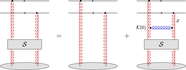
Figure 11: A graphical illustration of the integral version of the LO BK equation (36). Running-coupling corrections and non-linear effects in $\mathcal{S}$ describing multiple scattering are implicitly assumed, but not explicitly depicted.

We now introduce more schematic notations, as anticipated. Specifically, let us ignore (just in our notations) the transverse momentum convolutions, the inessential numerical factors, and the non-linear structure of functions like $\mathcal{J}$ w.r.t. the dipole $S$-matrix. Also, in writing the cross-section, we shall omit the quark distribution function. That is, we shall rewrite Eq. (3.3) simply as

$$\mathcal{N}_{{\rm\scriptscriptstyle LO}+{\rm\scriptscriptstyle NLO}}=\mathcal{S}_{0}+\Delta{\mathcal{S}}(X_{g})+\bar{\alpha}_{s}(k_{\perp}^{2})\int_{x_{g}}^{1}\frac{{\rm d}x}{x}\,\mathcal{K}(x)\,\mathcal{S}\big{(}X(x)\big{)}\,,$$ (34)

where the kernel $\mathcal{K}(x)$ encodes all the momentum space variables and convolutions (but no dipole $S$-matrix) and $\mathcal{S}\big{(}X(x)\big{)}$ succinctly denotes all the factors involving the dipole $S$-matrix, which could be either linear, or bi-linear, in $\mathcal{S}$. Both ‘real’ and ‘virtual’ contributions are implicitly added in the above integral. With these new notations, Eqs. (30) and (33) become

$${\mathcal{S}}(X_{g})={\mathcal{S}}_{0}+\Delta{\mathcal{S}}(X_{g})+\bar{\alpha}_{s}(k_{\perp}^{2})\int_{x_{g}}^{1}\frac{{\rm d}x}{x}\,\mathcal{K}(0)\,\mathcal{S}\big{(}X(x)\big{)}\,,$$ (35)

and respectively

$${\mathcal{S}}_{\rm\scriptscriptstyle rcBK}(X_{g})=\mathcal{S}_{0}+\bar{\alpha}_{s}(k_{\perp}^{2})\int_{x_{g}}^{1}\frac{{\rm d}x}{x}\,\mathcal{K}(0)\,\mathcal{S}_{\rm\scriptscriptstyle rcBK}\big{(}X(x)\big{)}\,,$$ (36)

where the kernel is now evaluated at $x=0$ (or $\xi=1$), that is, in the eikonal approximation. Clearly, the compact notation $\mathcal{K}(0)$ stays for the LO BK (or dipole) kernel. In particular, the rcBK equation (36) is graphically illustrated in Fig. 11.

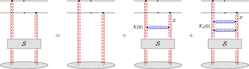
Figure 12: A graphical illustration of the integral version of the NLO BK equation (37). The middle term with kernel $\mathcal{K}(0)$ describes a soft gluon emission and corresponds to the LO BK kernel, but with a running coupling. The last term with kernel $\mathcal{K}_{2}(0)$ represents the NLO piece of the BK kernel, with the running-coupling corrections excluded. The two $s$-channel gluons included within $\mathcal{K}_{2}(0)$ can be close in rapidity. The non-linear effects in $\mathcal{S}$ describing multiple scattering are kept implicit.

These simpler notations hopefully make clear that the quantity denoted as $\Delta{\mathcal{S}}$ must encode all NLO corrections to the BK kernel except for those expressing the running of the coupling. These corrections should be computed in the large-$N_{c}$ limit, for consistency with our previous approximations. They can be inferred by inspection of the NLO version of the BK equation shown in Eq. (5) of Ref. Balitsky:2008zza . For convenience, we display the large-$N_{c}$ version of this equation in Appendix C, where we also discuss its collinear improvement, along the lines of Refs. Iancu:2015vea ; Iancu:2015joa . For simplicity, we shall stick here to our schematic notations and refer to Appendix C for more explicit formulae.

The integral version of the NLO BK equation reads (in momentum space and adapted to the kinematics at hand)

$${\mathcal{S}}(X_{g})={\mathcal{S}}_{0}+\bar{\alpha}_{s}(k_{\perp}^{2})\int_{x_{g}}^{1}\frac{{\rm d}x}{x}\,\mathcal{K}(0)\,\mathcal{S}\big{(}X(x)\big{)}+\bar{\alpha}_{s}^{2}(k_{\perp}^{2})\int_{x_{g}}^{1}\frac{{\rm d}x}{x}\,\mathcal{K}_{2}(0)\,\mathcal{S}\big{(}X(x)\big{)}\,,$$ (37)

where $\mathcal{K}_{2}(0)$ is a compact notation for the NLO piece of the BK kernel alluded to above: its action on $\mathcal{S}$ generates all the NLO terms visible in the r.h.s. of Eq. (C) except for the running coupling corrections, which are explicitly included in the middle term of Eq. (37). More precisely, if one uses the prescription (32) for the running coupling, then in constructing $\mathcal{K}_{2}(0)$ one should omit the NLO terms in Eq. (C) which are proportional to $\bar{b}$ (but keep all the other ones). Besides, the large NLO corrections enhanced by double or single collinear logarithms require all-order resummations (‘collinear improvement’), to be shortly described (see also the discussion in Appendix C).

By comparing Eqs. (35) and (37), it is now obvious that $\Delta{\mathcal{S}}(X_{g})$ must be identified with the third term in the r.h.s. of Eq. (37), that we now describe in some detail. As a general rule, the NLO corrections to the BK kernel are obtained by evaluating all the 2-loop graphs which yield a contribution of order $\alpha_{s}^{2}Y$ and hence count for a single step in the high-energy evolution (see Ref. Balitsky:2008zza for an exhaustive list of diagrams and explicit calculations). A typical such a graph involves a sequence of two gluon emissions, whose longitudinal fractions $x_{1}$ and $x_{2}$ obey $x_{1}\sim x_{2}\ll 1$; that is, the two gluons have similar rapidities, but they are both soft compared to the projectile. The integration variable $x$ in the last term in Eq. (37) can be interpreted as $x\equiv x_{1}+x_{2}$. The other independent rapidity integration, say over the variable $u\equiv x_{2}/(x_{1}+x_{2})$ with $0<u\leq 1$, is implicitly included in the structure of the NLO kernel $\mathcal{K}_{2}(0)$. This is possible since the scattering between the 2-gluon system and the target is independent of $u$ to the accuracy of interest. A rather schematic, but intuitive, graphical illustration of Eq. (37) is shown in Fig. 12.

At large $N_{c}$, two successive gluon emissions from the original $q\bar{q}$ dipole can generate up to three dipoles in the fundamental representation. Accordingly, the third term in Eq. (37) involves contributions which are cubic in the dipole $S$-matrix, together with quadratic and linear terms. All these contributions are visible in Eq. (C). To the accuracy of interest, the kinematics of the primary gluon (with energy fraction $x=x_{1}+x_{2}$) can be treated in the LLA. This explains why we were able to use the same lower limit $x_{g}$ in the integral over $x$ and also the same rapidity variable $X(x)$ for the relevant $S$-matrices as in the middle term in Eq. (37), which encodes the LO evolution.

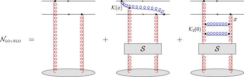
Figure 13: A graphical illustration of the factorization of quark production at NLO, as schematically encoded in Eq. (38). The primary gluon emission, with kernel $\mathcal{K}(x)$, is included with exact kinematics. The evolution step depicted as two-gluon emission with kernel $\mathcal{K}_{2}(0)$ succinctly represents the NLO piece of the BK kernel (but without the running-coupling corrections, which were already included in the middle term). Non-linear effects in $\mathcal{S}$, corresponding to multiple scattering, are implicitly included but not explicitly shown.

To conclude, the result for the quark multiplicity which is complete to NLO accuracy can be compactly, but schematically, written as

$$\mathcal{N}_{{\rm\scriptscriptstyle LO}+{\rm\scriptscriptstyle NLO}}=\mathcal{S}_{0}+\bar{\alpha}_{s}(k_{\perp}^{2})\int_{x_{g}}^{1}\frac{{\rm d}x}{x}\,\mathcal{K}(x)\,\mathcal{S}\big{(}X(x)\big{)}+\bar{\alpha}_{s}^{2}(k_{\perp}^{2})\int_{x_{g}}^{1}\frac{{\rm d}x}{x}\,\mathcal{K}_{2}(0)\,\mathcal{S}\big{(}X(x)\big{)}\,,$$ (38)

and is illustrated in Fig. 13. To deduce a more explicit expression, one should use Eq. (3.3) together with the formula for $\Delta\mathcal{S}$ shown in Appendix C.

Although the above factorization scheme is formally correct to NLO, it might be still too hard, if not impossible, to achieve a full NLO accuracy in a practical calculation. Indeed, as already mentioned, the target evolution is not known to NLO and the relation between the function $\mathcal{S}\big{(}X(x)\big{)}$ which enters the above factorization and the solution $\mathcal{S}(x)$ to the NLO BK equation for the projectile is not known at the accuracy of interest. Besides, numerical calculations might be hindered by the complexity of the NLO BK equation and of the transverse convolutions implicit in the two integral terms in Eq. (38). In view of that, we would like to propose two approximation schemes which we believe have more chances to be transposed in practice. In both schemes, the approximations refer to the dipole evolution, whereas the NLO impact factor, as represented by the kernel $\mathcal{K}(x)$ in the middle term in Eq. (38), should be treated exactly.

The simplest approximation which is still physically meaningful is the LO approximation (in the sense of rcBK) to the dipole evolution. This is obtained by neglecting the third term in Eq. (38) and replacing $\mathcal{S}\simeq\mathcal{S}_{\rm\scriptscriptstyle rcBK}$ within the integrand of the middle term. A similar strategy has been used Stasto:2013cha ; Stasto:2014sea ; Watanabe:2015tja in relation with the ‘plus’ prescription Chirilli:2011km ; Chirilli:2012jd ; the respective numerical calculations, albeit very complex, turned out to be tractable Zaslavsky:2014asa .

The second approximation, which is more ambitious, refers to the use of the collinearly-improved version of the BK equation, as proposed in Refs. Iancu:2015vea ; Iancu:2015joa . We recall that, besides the running coupling corrections, this equation also resums double-collinear logarithms together with a subset of the single collinear logarithms (which includes the respective contribution at NLO). The corresponding approximation to Eq. (38) involves two aspects. On the one hand, one must relate the function $\mathcal{S}\big{(}X(x)\big{)}$, which encodes the evolution of the target, to the solution to the collinearly-improved BK equation (which refers to the evolution of the projectile). This aspect is particularly important for the middle term in Eq. (38) and will be discussed in Appendix B. On the other hand, one must use a simplified version of the NLO BK kernel $\mathcal{K}_{2}(0)$ which keeps only those corrections to the LO kernel which refer to the collinear improvement. This will be described in what follows.

To that aim, it is convenient to use the coordinate representation: the last term in Eq. (38), which we recall corresponds to the piece $\Delta{\mathcal{S}}(\bm{k},X_{g})$ in Eq. (3.3), will be written as

$$\Delta{\mathcal{S}}(\bm{k},X_{g})=\int{\rm d}^{2}\bm{r}\,{\rm e}^{-{\rm i}\bm{k}\cdot\bm{r}}{\Delta S}(\bm{r},x_{\rm\scriptscriptstyle T})\,,$$ (39)

where $\bm{r}=\bm{x}-\bm{y}$ and

$${\Delta S}(\bm{x},\bm{y};x_{\rm\scriptscriptstyle T})\equiv\int_{x_{\rm\scriptscriptstyle T}}^{1}\frac{{\rm d}x}{x}\int\frac{{\rm d}^{2}\bm{z}}{2\pi}\,\bar{\alpha}_{\rm fac}\,{\mathcal{M}}_{\bm{x}\bm{y}\bm{z}}\big{(}\mathcal{K}_{{\rm\scriptscriptstyle DLA}}\mathcal{K}_{{\rm\scriptscriptstyle SL}}-1\big{)}\Big{[}S\Big{(}\bm{x},\bm{z};\frac{x_{\rm\scriptscriptstyle T}}{x}\Big{)}S\Big{(}\bm{z},\bm{y};\frac{x_{\rm\scriptscriptstyle T}}{x}\Big{)}-S\Big{(}\bm{x},\bm{y};\frac{x_{\rm\scriptscriptstyle T}}{x}\Big{)}\Big{]}.$$ (40)

In the above equation, we recognize the dipole kernel ${\mathcal{M}}_{\bm{x}\bm{y}\bm{z}}$ and the running coupling $\bar{\alpha}_{\rm fac}$ that were introduced before, together with two multiplicative corrections to the kernel, $\mathcal{K}_{{\rm\scriptscriptstyle DLA}}$ and $\mathcal{K}_{{\rm\scriptscriptstyle SL}}$, which encode the resummations of double and respectively single collinear logarithms, as alluded to above. Physicswise, $\mathcal{K}_{{\rm\scriptscriptstyle DLA}}$ implements the condition of time-ordering for the successive soft gluon emissions by the projectile, whereas $\mathcal{K}_{{\rm\scriptscriptstyle SL}}$ resums a subset of the DGLAP logarithms (see Refs. Iancu:2015vea ; Iancu:2015joa for details). The new rapidity argument $x_{\rm\scriptscriptstyle T}$ which appears too in Eq. (40) will be later explained.

Specifically, $\mathcal{K}_{{\rm\scriptscriptstyle DLA}}$ is defined as the function

$$\mathcal{K}_{{\rm\scriptscriptstyle DLA}}(\rho)=\frac{{\rm J}_{1}\big{(}2\sqrt{\bar{\alpha}_{s}\rho^{2}}\big{)}}{\sqrt{\bar{\alpha}_{s}\rho^{2}}}=1-\frac{\bar{\alpha}_{s}\rho^{2}}{2}+\frac{(\bar{\alpha}_{s}\rho^{2})^{2}}{12}+\cdots,$$ (41)

evaluated at $\rho^{2}={L_{\bm{x}\bm{z}r}L_{\bm{y}\bm{z}r}}$, with $L_{\bm{x}\bm{z}r}\equiv\ln[(\bm{x}-\bm{z})^{2}/r^{2}]$. If the double logarithm $L_{\bm{x}\bm{z}r}L_{\bm{y}\bm{z}r}$ is negative, then one uses its absolute value and the Bessel function ${\rm J}_{1}$ gets replaced by the modified Bessel function ${\rm I}_{1}$. Note however that if, e.g., $(\bm{x}-\bm{z})^{2}\ll r^{2}$, so that $L_{\bm{x}\bm{z}r}<0$, then $(\bm{y}-\bm{z})^{2}\simeq r^{2}$ and hence $L_{\bm{y}\bm{z}r}\simeq 0$. Accordingly, the relatively small daughter dipoles bring no significant contributions to the difference $\mathcal{K}_{{\rm\scriptscriptstyle DLA}}-1$. Furthermore,

$$\mathcal{K}_{{\rm\scriptscriptstyle SL}}=\exp\left\{-\bar{\alpha}_{s}A_{1}\left|\ln\frac{(\bm{x}\!-\!\bm{y})^{2}}{\min\{(\bm{x}\!-\!\bm{z})^{2},(\bm{y}\!-\!\bm{z})^{2}\}}\right|\right\},\qquad A_{1}=\frac{11}{12}+\frac{N_{\rm f}}{6N_{\rm c}^{3}}\,,$$ (42)

where $A_{1}$ is the ‘gluonic anomalous dimension’ of the DGLAP evolution (see e.g. Ciafaloni:1999yw for details). Note that the difference $\mathcal{K}_{{\rm\scriptscriptstyle DLA}}\mathcal{K}_{{\rm\scriptscriptstyle SL}}-1$ starts at $\mathcal{O}{(\bar{\alpha}_{s})}$, as expected. However, keeping only that lowest-order term in the expansion would artificially enhance the importance of the ‘collinear’ regions in phase-space — the regions where the successive gluon emissions (or dipole splittings) are strongly ordered in transverse sizes, or momenta. This is the origin of the instability of the strict NLO approximation to the high-energy evolution, as previously mentioned.

Vice-versa, the all-order resummation of such corrections within the factor $\mathcal{K}_{{\rm\scriptscriptstyle DLA}}\mathcal{K}_{{\rm\scriptscriptstyle SL}}$ suppresses the contributions from the ‘collinear’ regions and thus restores the convergence of perturbation theory. This is rather obvious for the second factor $\mathcal{K}_{{\rm\scriptscriptstyle SL}}$, which exponentially cuts off the configurations where the daughter dipoles are either much smaller, or much larger, than the parent dipole. But this is also true for the other factor $\mathcal{K}_{{\rm\scriptscriptstyle DLA}}$, which, as already mentioned, becomes important only when the daughter dipoles are sufficiently large, such that $\bar{\alpha}_{s}\rho^{2}\gg 1$. In that case, the Bessel function ${\rm J}_{1}\big{(}2\sqrt{\bar{\alpha}_{s}\rho^{2}}\big{)}$ is rapidly oscillating when varying the position $\bm{z}$ of the emitted gluon, hence the integral over the regions in space where ‘$\bm{z}$ is large’ (in the sense that $|\bm{z}-\bm{x}|\sim|\bm{z}-\bm{y}|\gg r$) averages to zero.

To conclude, for gluon emissions which are strongly ordered in transverse momenta, we have $\mathcal{K}_{{\rm\scriptscriptstyle DLA}}\mathcal{K}_{{\rm\scriptscriptstyle SL}}\simeq 0$ and then the overall kernel in Eq. (40) reduces to minus the LO kernel $-\mathcal{K}(0)$. In turn, the latter subtracts the soft and collinear contributions to the middle term in Eq. (38), that is, it implements the collinear improvement for the LO evolution, as it should.

There is one more aspect of Eq. (40) which requires a few words of explanation: the rapidity arguments of the various $S$-matrices and, related to them, the lower limit $x_{\rm\scriptscriptstyle T}$ for the integral over $x$. If the evolution of these $S$-matrices is computed to LO, i.e. according to rcBK, then one can identify $x_{\rm\scriptscriptstyle T}\simeq x_{g}=k_{\perp}^{2}/\hat{s}$ and there is no distinction between projectile and target evolutions. Albeit such an approximation would be formally justified to NLO accuracy, it is still preferable to use the collinearly-improved evolution, i.e. the BK equation with the resummed kernel ${\mathcal{M}}_{\bm{x}\bm{y}\bm{z}}\mathcal{K}_{{\rm\scriptscriptstyle DLA}}\mathcal{K}_{{\rm\scriptscriptstyle SL}}$. Indeed, this would ensure a smooth matching with the middle term in Eq. (38), where the collinearly-improved version of the evolution becomes compulsory. Since the latter has been formulated for projectile evolution alone Iancu:2015vea ; Iancu:2015joa , one must understand what is the longitudinal phase-space for the evolution in $x=q^{+}/q_{0}^{+}$ which corresponds to the physical range for the evolution in $X=q^{-}/P^{-}$. In coordinate space and to the accuracy of interest, one can write (see e.g. Iancu:2015vea )

$$S_{\rm\scriptscriptstyle T}\big{(}\bm{r},X\big{)}=S_{\rm\scriptscriptstyle P}\big{(}\bm{r},x_{\rm\scriptscriptstyle T}\big{)}\,\qquad\mbox{with}\qquad X=\frac{Q^{2}}{\hat{s}}\,\gg\,x_{\rm\scriptscriptstyle T}=\frac{Q^{2}_{0}}{\hat{s}}\,,$$ (43)

where we have temporarily introduced the subscripts T (‘target’) and P (‘projectile’), to make the discussion more transparent and we recall that $\hat{s}=2q_{0}^{+}P^{-}$. In this equation, $Q=1/r$ is the dipole resolution scale in the transverse plane and can be also identified with the transverse momentum $k_{\perp}$ of the produced quark, via the Fourier transform (39); hence, $X\simeq X_{g}=x_{g}$. Furthermore, $Q_{0}$ is the saturation scale in the nuclear target at low energy (say, within the MV model). The interesting situation is such that $k_{\perp}\gtrsim Q_{s}(X_{g})\gg Q_{0}$ and therefore $x_{\rm\scriptscriptstyle T}\ll x_{g}$, as indicated too in Eq. (43).

The relation (43) can be understood as follows. The scattering between the small dipole and the nuclear target probes the evolution of the latter down to values of $X$ such that the longitudinal extent $\Delta x^{+}=1/(XP^{-})$ of the softest target fluctuations is still smaller than the lifetime $2q_{0}^{+}/Q^{2}$ of the dipole projectile. This argument, which selects $X={Q^{2}}/{\hat{s}}$ as anticipated, is merely a variation of our earlier derivation of Eq. (1) in Sect. 2.1. If on the other hand the evolution is encoded in the wavefunction of the projectile, then one should allow for the small-$x$ fluctuations with transverse momenta $\bm{q}$ within the range $Q^{2}>q_{\perp}^{2}>Q_{0}^{2}$ and with large enough lifetimes $2xq_{0}^{+}/q_{\perp}^{2}\gtrsim 1/P^{-}$ (indeed, $1/P^{-}$ is the longitudinal extent of the un-evolved target). These conditions imply $x\gtrsim q_{\perp}^{2}/\hat{s}\geq Q_{0}^{2}/\hat{s}$, or $x\geq x_{\rm\scriptscriptstyle T}$, which explains the lower limit in the integral over $x$ in Eq. (40).

One may find surprising that the rapidity interval $\Delta y=\ln(1/x_{\rm\scriptscriptstyle T})$ available for the evolution of the projectile is much larger than that, $\Delta Y=\ln(1/X_{g})$, allowed for the evolution of the target. But one should keep in mind that the projectile evolution with decreasing $x$ is strongly constrained by the condition of time-ordering, which limits the corresponding transverse phase-space (via the multiplicative correction $\mathcal{K}_{{\rm\scriptscriptstyle DLA}}$ to the kernel) and thus reduces the evolution speed. By contrast, there is no similar constraint for the evolution of the target with decreasing $X$, since in that case the physical condition of time-ordering is automatically satisfied.

3.5 Subtracting the leading order evolution: why is this subtle

The factorization scheme that we have constructed in the previous sections, cf. Eqs. (3.3) or (38), does not involve any subtraction: there is no over-counting of the relevant perturbative contributions and hence no need for a subtraction. We therefore expect that calculations based on this factorization should yield a positive result for the quark multiplicity. More explicit arguments in that sense will be presented later in this section. This represents a significant improvement over the previous proposal in Refs. Chirilli:2011km ; Chirilli:2012jd , so it is interesting to better understand the relation between these two schemes.

From the discussion in Sect. 3.1, we recall that in the approach Chirilli:2011km ; Chirilli:2012jd on explicitly subtracts the LO evolution of the dipole $S$-matrix from the NLO correction to the impact factor. Such a subtraction can also be performed within our present approach. To synthetically describe that, we shall again use the schematic notations introduced in the previous subsection. Using Eq. (37), we can express the last term in the NLO cross-section (38) (a NLO correction to the dipole evolution) as the difference between the dipole $S$-matrix at NLO and its LO evolution:

$$\bar{\alpha}_{s}^{2}(k_{\perp}^{2})\int_{x_{g}}^{1}\frac{{\rm d}x}{x}\,\mathcal{K}_{2}(0)\mathcal{S}\big{(}X(x)\big{)}={\mathcal{S}}(X_{g})-\left[{\mathcal{S}}_{0}+\bar{\alpha}_{s}(k_{\perp}^{2})\int_{x_{g}}^{1}\frac{{\rm d}x}{x}\,\mathcal{K}(0)\,\mathcal{S}\big{(}X(x)\big{)}\right]\,.$$ (44)

The r.h.s. of this equation is not exactly the same as the difference $\mathcal{S}-\mathcal{S}_{\rm\scriptscriptstyle rcBK}$, but it is very close to it. (The expression between the square brackets would reduce to $\mathcal{S}_{\rm\scriptscriptstyle rcBK}$ if the $S$-matrix under the integral would be itself approximated by rcBK; recall Eq. (47).) So, clearly, Eq. (44) expresses a NLO correction which is a priori small as the difference between two quantities which are individually large: each of them includes the LO contribution $\mathcal{S}_{\rm\scriptscriptstyle rcBK}$. Inserting Eq. (44) into Eq. (38), one deduces an alternative expression for the NLO cross-section,

$$\mathcal{N}_{{\rm\scriptscriptstyle LO}+{\rm\scriptscriptstyle NLO}}=\mathcal{S}(X_{g})\,+\bar{\alpha}_{s}(k_{\perp}^{2})\int_{x_{g}}^{1}\frac{{\rm d}x}{x}\,\big{[}\mathcal{K}(x)-\mathcal{K}(0)\big{]}\,\mathcal{S}\big{(}X(x)\big{)},$$ (45)

in which the LO evolution (as represented by the kernel $\mathcal{K}(0)$) is explicitly subtracted from the impact factor. Since the difference $\mathcal{K}(x)-\mathcal{K}(0)$ vanishes as $x\to 0$, the above integral is controlled by large values $x\sim 1$ and it does not generate a small-$x$ logarithm anymore. That is, the second term in the r.h.s. of Eq. (45) is a pure $\bar{\alpha}_{s}$ correction, that can be viewed as the NLO contribution to the impact factor. The NLO correction to the dipole evolution is now fully encoded in the first term $\mathcal{S}(X_{g})$. Indeed, to the NLO accuracy of interest, the $S$-matrix within the integral can be evaluated by using the LO approximation, $\mathcal{S}\simeq\mathcal{S}_{\rm\scriptscriptstyle rcBK}$.

Eq. (45) is very similar to the proposal in Refs. Chirilli:2011km ; Chirilli:2012jd , which in our schematic notations reads

$$\mathcal{N}_{{\rm\scriptscriptstyle CXY}}=\mathcal{S}(X_{g})+\bar{\alpha}_{s}(k_{\perp}^{2})\int_{0}^{1}\frac{{\rm d}x}{x}\,\big{[}\mathcal{K}(x)-\mathcal{K}(0)\big{]}\,\mathcal{S}(X_{g})\,.$$ (46)

The main difference w.r.t. Eq. (45) is that the $S$-matrix within the above integral over $x$ is not evaluated at the $x$-dependent rapidity argument $X(x)$, but rather at its endpoint value $X_{g}=X(1)$. In other terms, Eq. (46) is local in the target rapidity $X_{g}$, as standard for the $k_{\perp}$-factorization. In spite of this difference, the results in Eqs. (46) and (45) are perturbatively equivalent to NLO accuracy. Indeed, since the integral over $x$ in (45) is controlled by $x\sim 1$, there is no loss of NLO accuracy if one replaces $\mathcal{S}\big{(}X(x)\big{)}\to\mathcal{S}(X_{g})$. This can be easily checked by using the dominant energy-behavior of the BK solution in the weak scattering regime, namely $\mathcal{S}(X)\propto 1/X^{\lambda}$ with $\lambda=\mathcal{O}{(\bar{\alpha}_{s})}$.

This being said, one should keep in mind that the limiting value $\mathcal{S}(X_{g})$ is strictly larger than $\mathcal{S}\big{(}X(x)\big{)}$ for any $x<1$, because the function $\mathcal{S}(X)$ increases when decreasing $X$. Hence, albeit formally allowed to the accuracy of interest, the replacement $\mathcal{S}\big{(}X(x)\big{)}\to\mathcal{S}(X_{g})$ could still be troublesome, in that it might result in an over-subtraction. Indeed, as discussed in Ducloue:2016shw , the difference $\mathcal{K}(x)-\mathcal{K}(0)$ is strictly negative for sufficiently large $k_{\perp}\gtrsim Q_{s}$. Hence, the negative correction to the impact factor at large $k_{\perp}$ is over included in (46) as compared to (45), a feature which might contribute to the ‘negativity’ problem under consideration.

In order to discuss this problem — the fact that the cross-section computed according to Eq. (46) becomes negative at sufficiently large (but still semi-hard) $k_{\perp}$ —, it is useful to keep in mind that previous numerical evaluations of Eq. (46) used approximate versions of the dipole $S$-matrix, like $\mathcal{S}_{\rm\scriptscriptstyle rcBK}$ Stasto:2013cha ; Stasto:2014sea ; Watanabe:2015tja . Hence, it would be interesting to understand why Eq. (46) with $\mathcal{S}\to\mathcal{S}_{\rm\scriptscriptstyle rcBK}$ can lead to a negative cross-section at large transverse momenta.

To that aim, let us consider the rcBK approximation to the ‘subtracted’ version of our factorization scheme, cf. (45). This reads

$$\mathcal{N}_{{\rm\scriptscriptstyle rcBK}}=\mathcal{S}_{{\rm\scriptscriptstyle rcBK}}+\bar{\alpha}_{s}(k_{\perp}^{2})\int_{x_{g}}^{1}\frac{{\rm d}x}{x}\,\big{[}\mathcal{K}(x)-\mathcal{K}(0)\big{]}\,\mathcal{S}_{\rm\scriptscriptstyle rcBK}\big{(}X(x)\big{)}\,.$$ (47)

Via the rcBK equation (36), this is equivalent to

$$\mathcal{N}_{{\rm\scriptscriptstyle rcBK}}=\mathcal{S}_{0}+\bar{\alpha}_{s}(k_{\perp}^{2})\int_{x_{g}}^{1}\frac{{\rm d}x}{x}\,\mathcal{K}(x)\,\mathcal{S}_{\rm\scriptscriptstyle rcBK}\big{(}X(x)\big{)},$$ (48)

which is of course the same as our ‘un-subtracted’ result in Eq. (34) with $\Delta\mathcal{S}=0$ and $\mathcal{S}\to\mathcal{S}_{\rm\scriptscriptstyle rcBK}$.

We believe that the r.h.s. of Eq. (48) should be positive. Indeed, when the primary gluon emission is treated in the eikonal approximation ($\mathcal{K}(x)\to\mathcal{K}(0)$), Eq. (48) is the same as the integral representation of $\mathcal{S}_{\rm\scriptscriptstyle rcBK}$, which is well known to be positive definite (at least in coordinate space). With the actual kernel $\mathcal{K}(x)$, the value of the integral term should be somewhat reduced (since the correct phase-space for the primary gluon emission is smaller than its eikonal estimate), but this should remain positive, as it describes the growth of the dipole $S$-matrix via gluon emissions.

Hence, the ‘subtracted’ result in Eq. (47) should be positive as well. In spite of that, we believe that explicit numerical calculations based on Eq. (47) may run into difficulties (in particular, yield a negative result) because of the high degree of ‘fine-tuning’ inherent in the subtraction method: in going from Eq. (48) to Eq. (47), we have added and subtracted the same quantity ($\mathcal{S}_{\rm\scriptscriptstyle rcBK}$), but we have done that in a very peculiar way: we have added the l.h.s. of Eq. (36), that is, $\mathcal{S}_{\rm\scriptscriptstyle rcBK}$ itself, but we have subtracted the r.h.s. of Eq. (36), that is, the integral representation of $\mathcal{S}_{\rm\scriptscriptstyle rcBK}$. This procedure leaves the result unchanged if and only if the function $\mathcal{S}_{\rm\scriptscriptstyle rcBK}$ is an exact solution to the integral equation (36). But any numerical approximation in solving rcBK, or in the Fourier transform $S(\bm{r},X)\to\mathcal{S}(\bm{k},X)$, may lead to an imbalance between the terms that have been added and respectively subtracted.

For instance, such an imbalance could be introduced by the treatment of the running coupling corrections, which in general is not fully coherent between the coordinate-space and the momentum-space representations. In practice, the momentum-space version of the rcBK equation, as shown in (36), is not the exact Fourier transform of the respective equation in coordinate space: the Fourier transform is not also applied to the running of the coupling. So, strictly speaking, there is some mismatch between Eqs.  (47) and (48) even when using the exact solution to the rcBK equation, as obtained in coordinate space. When computing the cross-section according to Eq. (46), this mismatch can be further enhanced by the fact that the function $\mathcal{S}_{\rm\scriptscriptstyle rcBK}\big{(}X(x)\big{)}$ gets replaced by its maximal value $\mathcal{S}_{\rm\scriptscriptstyle rcBK}(X_{g})$ (cf. the discussion after Eq. (46)).

From the above discussion, we see that the rcBK equation plays the role of a ‘self-consistency condition’ for rewriting the cross-section in a ‘subtracted’ form. To illustrate the importance of having ‘good’ solutions to this equation, let us consider a somewhat extreme example, where this condition is strongly violated. (A similar discussion can be found in Ducloue:2016shw .) Namely, we consider the popular approximation in which the dipole $S$-matrix is taken from the GBW model GolecBiernat:1998js , which is a Gaussian:

$${\mathcal{S}}_{\rm\scriptscriptstyle GBW}(\bm{k},X)\,=\,\frac{4\pi}{Q_{s}^{2}}\,{\rm e}^{-\frac{k_{\perp}^{2}}{Q_{s}^{2}}}\,,$$ (49)

where $Q_{s}^{2}(X)=Q_{0}^{2}(X_{0}/X)^{\lambda}$ with $\lambda\simeq 0.3$. Clearly, this is a very poor approximation at high $k_{\perp}\gtrsim Q_{s}$, where it decays exponentially, in sharp contrast with the power law tail $1/k_{\perp}^{4}$ predicted by pQCD. Using this particular model within Eq. (45), one finds

$$\mathcal{N}_{{\rm\scriptscriptstyle GBW}}=\mathcal{S}_{{\rm\scriptscriptstyle GBW}}(X_{g})+\bar{\alpha}_{s}\int_{x_{g}}^{1}\frac{{\rm d}x}{x}\,\big{[}\mathcal{K}(x)-\mathcal{K}(0)\big{]}\,\mathcal{S}_{\rm\scriptscriptstyle GBW}\big{(}X(x)\big{)}\,.$$ (50)

The ‘LO’ piece $\mathcal{S}_{{\rm\scriptscriptstyle GBW}}$ exponentially vanishes at large $k_{\perp}\gg Q_{s}$, whereas the ‘subtracted’ piece shows a tail $\propto 1/k_{\perp}^{4}$, since obtained by iterating once the LO BK equation. So, the ‘subtracted’ piece is not only larger than the ‘LO’ one, but it is the only one to survive at large $k_{\perp}$. Hence, at $k_{\perp}\gtrsim Q_{s}$ the overall result reduces to the second, ‘NLO’, piece, which is negative in that particular region of phase-space Ducloue:2016shw , as already mentioned. This is in agreement with the numerical findings in Watanabe:2015tja ; Ducloue:2016shw .

To summarize, albeit Eqs. (47) and (48) are in principle equivalent with each other, the second equation is probably safer to use in practice. A similar discussion applies to the full NLO cross-section: the ‘unsubtracted’ factorization (38) should provide a meaningful result which is positive when evaluated with either the NLO $S$-matrix $\mathcal{S}$, or with its collinearly-improved version $\mathcal{S}_{{\rm\scriptscriptstyle collBK}}$. On the other hand, the ‘subtracted’ version (45), which may look appealing since structurally simpler, is likely to be more tricky to use in practice.

4 Summary and conclusions

In this paper, we have established a factorization scheme allowing the computation of single-inclusive particle production at forward rapidities in proton-nucleus collisions at next-to-leading order in pQCD, in the presence of the non-linear effects associated with the high gluon density in the nuclear target. The main difference with respect to the previous proposal in Chirilli:2011km ; Chirilli:2012jd is that our result involves no rapidity subtraction, meaning that it is free of the fine-tuning problem inherent in any such a subtraction scheme. The ‘fine-tuning’ refers to the fact that the numerical solution to the evolution equation for the dipole $S$-matrix must be precisely known to ensure that the quantity which is included as ‘LO evolution’ is properly subtracted from the ‘NLO correction to the impact factor’. Further approximations within the subtraction scheme, which are formally allowed to NLO accuracy, or even small numerical errors in the associated calculations, may spoil such a fine cancellation and lead to unphysical results. In our opinion, this is the reason why the cross-section computed within this scheme appears to turn negative at sufficiently large transverse momenta Stasto:2013cha ; Stasto:2014sea ; Watanabe:2015tja ; Ducloue:2016shw . By contrast, our scheme is more robust and should converge to physical, positive-definite, results with considerably less numerical efforts.

Our factorization scheme relies on the skeleton structure of perturbative QCD up to two-loop order, which is the relevant loop-order for the NLO calculation. The most general version of our result is exhibited in Eq. (3.2). This version however is probably too complicated to be used in practice. Fortunately, important simplifications become possible in the interesting situation where the transverse momentum $k_{\perp}$ of the produced quark is relatively large, $k_{\perp}\gtrsim Q_{s}$. In that case, the primary gluon is hard as well, $p_{\perp}\sim k_{\perp}$, and the general formula (3.2) can be then replaced by Eq. (3.3) [or (3.3)], which is considerably simpler. The latter shows the same degree of complexity, in terms of transverse integrations, like the formulae already used in practice in relation with the subtraction method. So, we are confident that Eq. (3.3) can indeed by explicitly evaluated, via the numerical tools developed in Zaslavsky:2014asa ; Stasto:2013cha ; Stasto:2014sea ; Watanabe:2015tja ; Ducloue:2016shw . As discussed in Sect. 2.4, the fact that we can approximate $p_{\perp}\sim k_{\perp}$ is specific to the problem of particle production. This would not apply, say, to deep inelastic scattering, where the dipole evolution must be computed in transverse coordinate space. In that case, if the parent dipole is sufficiently small ($r\ll 1/Q_{s}$) — as appropriate for DIS at relatively high virtuality $Q^{2}\gg Q_{s}^{2}$ —, then the first gluon emission in the high-energy evolution is considerably softer (it typically carries a transverse momentum $p_{\perp}\ll 1/r$) and the dependence upon its transverse kinematics cannot be simplified at NLO. This is visible in the NLO calculations of the DIS impact factor Balitsky:2010ze ; Beuf:2011xd ; Balitsky:2012bs ; Beuf:2016wdz .

To explicitly evaluate the quark multiplicity according to Eq. (3.3), one also needs a suitable approximation for the high-energy evolution of the dipole $S$-matrix. The simplest such an approximation which is still meaningful for phenomenology is the LO BK equation with running coupling (rcBK) Kovchegov:2006wf ; Kovchegov:2006vj ; Balitsky:2006wa . A more accurate treatment of the evolution can be obtained by using the collinearly-improved BK equation Beuf:2014uia ; Iancu:2015vea ; Iancu:2015joa ; Albacete:2015xza ; Lappi:2016fmu ; Hatta:2016ujq , which resums the double collinear logarithms inherent in the ‘hard-to-soft’ evolution of the projectile together with a subset of single collinear logs. The inclusion of the collinear improvement in the problem at hand is quite subtle, due to the need to properly identify the rapidity phase-space for the evolution of the dilute projectile (the incoming quark, or the pair made with this quark and the hard primary gluon). This is clarified in Sect. 3.4 and Appendix B.

An important lesson emerging from our analysis is that one should not always insist in writing the result of a NLO calculation in pQCD at high-energy in a ‘$k_{\perp}$-factorized form’, which is local in rapidity. This can be best appreciated by comparing our results in Eqs. (38), (45), and (46). Eq. (38) is obtained via a direct evaluation of the relevant, one-loop and two-loop, diagrams. As such, it does not involve any rapidity subtraction at one-loop level: the would-be NLO correction to the impact factor and the first step in the high-energy evolution of the color dipole are both encoded in the middle term in Eq. (38). In Eq. (45), the two contributions that we just mentioned are explicitly separated from each other, via a rapidity subtraction, but the result is still not ‘factorized’: the $\mathcal{O}{(\alpha_{s})}$-correction to the impact factor and the dipole $S$-matrix are still entangled by the rapidity integral over $x$ (besides the transverse momentum convolutions which are implicit in our schematic notations). Finally, Eq. (46) expresses a genuine $k_{\perp}$-factorization: the r.h.s. is local in the target rapidity $X_{g}$ and the NLO impact factor is explicitly factorized (in so far as the rapidity dependence is concerned) from the dipole $S$-matrices, which encode the high-energy evolution. These three representations for the NLO cross-section, (38), (45), and (46), are all consistent with each other to NLO accuracy. Yet, the two representations involving a rapidity subtraction, Eqs. (45) and (46), are potentially affected by the issue of fine-tuning that we have identified in this paper. By contrast, the original result in Eq. (38) is free from this problem and therefore it should provide a positive-definite estimate for the cross-section.

We would like to conclude this section with some prospects for the extension of this factorization program beyond NLO. Our factorization scheme suggests an interesting pattern which is likely to survive beyond the present approximations. The distinguished feature of this pattern is the fact that the higher-order corrections to the impact factor are not explicitly separated from the relevant corrections to the high-energy evolution. To illustrate this point, let us consider quark production at NNLO. Without any claim to completeness and leaving aside the possibility of new contributions which go beyond the dipole picture, let us here indicate the generic structure that we expect in view of our previous analysis in this paper. Namely, we expect the NNLO cross-section to include the following four terms (in schematic notations, similar to those introduced in Sect. 3.4)

$$\mathcal{N}_{{\rm\scriptscriptstyle LO}+{\rm\scriptscriptstyle NLO}+{\rm\scriptscriptstyle NNLO}}=\mathcal{S}_{0} +\bar{\alpha}_{s}(k_{\perp}^{2})\int_{x_{g}}^{1}\frac{{\rm d}x}{x}\,\mathcal{K}(x)\,\mathcal{S}\big{(}X(x)\big{)}$$

$$+\bar{\alpha}_{s}^{2}(k_{\perp}^{2})\int_{x_{g}}^{1}\frac{{\rm d}x_{1}}{x_{1}}\int_{x_{g}}^{x_{1}}\frac{{\rm d}x_{2}}{x_{2}}\,\big{[}\mathcal{K}_{2}(x_{1},x_{2}/x_{1})-\mathcal{K}_{2}(x_{1},0)\big{]}\,\mathcal{S}\big{(}X(x_{1},x_{2})\big{)}$$

$$+\bar{\alpha}_{s}^{3}(k_{\perp}^{2})\int_{x_{g}}^{1}\frac{{\rm d}x}{x}\,\mathcal{K}_{3}(0)\,\mathcal{S}\big{(}X(x)\big{)}\,,$$ (51)

where it is now understood that the dipole $S$-matrices evolve according to the (presently unknown) NNLO version of the BK equation. The argument of the running couplings is taken as $k_{\perp}^{2}$, for illustration, but this should be the right choice only in the limit where the transverse momentum of the produced quark is larger than any other transverse scale in the problem. Also, the lower limit $x_{g}$ on the integrals over $x$ is purely illustrative: the actual limit should depend upon the exact kinematics. The first two terms in the r.h.s. of Eq. (4) have the same structure as the respective terms in Eq. (38); in particular, the second term encodes the NLO impact factor and the LO piece of the BK kernel. The third term is a generalization of the last term in Eq. (38): it encodes the NLO piece of the BK kernel together with the NNLO correction to the impact factor. This term is generated by 2-loop graphs where the 2 emitted partons (say, gluons) can have arbitrarily energy fractions $x_{1}$ and $x_{2}$ (with $x_{2}\leq x_{1}$ for definiteness), so their emissions must be computed with exact kinematics. The sum of all such graphs is schematically represented by the kernel $\mathcal{K}_{2}(x_{1},x_{2}/x_{1})$. The subtraction of $\mathcal{K}_{2}(x_{1},0)$ is needed to avoid the over inclusion of the first two steps in the high energy evolution, that were already included in the second term, with kernel $\mathcal{K}(x)$. Finally, the fourth term in Eq. (4) represents the NNLO correction to the BK kernel, as generated by 3-loop graphs in which the 3 gluons are all soft, but close in rapidity to each other: $x_{1}\sim x_{2}\sim x_{3}\ll 1$. Clearly, in the limit where the very first emission by the projectile is soft and computed in the eikonal approximation, the r.h.s. of Eq. (4) becomes proportional to the integral representation of the NNLO BK equation.

Appendix A Cancellation of shortly lived virtual fluctuations

As we have seen, the minus longitudinal momentum $p^{-}=p_{\perp}^{2}/2p^{+}$ of the primary gluon is constrained by light-cone energy conservation, that is, by Eq. (8). This constraint however exists only for the gluons which are crossing the cut (albeit eventually non measured), but not also for those which are emitted and reabsorbed on the same side of the cut. In principle, such ‘virtual’ gluons are allowed to have very short lifetimes $2p^{+}/p_{\perp}^{2}<1/P^{-}$, however we shall show here that their respective contributions cancel exactly. To that aim, we shall separately consider the two possible regimes in terms of the ratio $p_{\perp}/k_{\perp}$. We recall that $k_{\perp}$ is the transverse momentum of the measured quark and for the virtual diagrams it coincides with the momentum transferred by the target via scattering.

(i) $p_{\perp}\gg k_{\perp}$. This is the simplest case, as the virtual fluctuation cannot be resolved by the scattering (the transverse separation $\Delta x_{\perp}\sim 1/p_{\perp}$ between the virtual gluon and its parent quark is much smaller than the transverse resolution $\sim 1/k_{\perp}$ of the exchanged gluon). Accordingly, all the diagrams shown in Fig. 14 are equally weighted by the $S$-matrix, so their sum must vanish by probability conservation. In practice, this occurs because the two self-energy graphs in figures (a) and (c) have a different sign as compared to the vertex correction in figure (b) and also an additional factor 1/2.

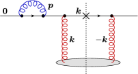
(a)

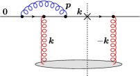
(b)

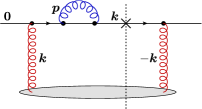
(c)

Figure 14: The virtual diagrams when $p_{\perp}\gg k_{\perp}$. In such a regime the shortly lived $p$-line is attached only to the projectile quark and the sum of the diagrams vanishes due to probability conservation. Transverse momenta are shown in the graphs.

(ii) $p_{\perp}\lesssim k_{\perp}$. This case is much less trivial than (i), since now one has to also consider the diagrams in which the virtual gluon with momentum $p$ is emitted and/or absorbed by the exchanged gluon. For the calculation that follows, it is convenient to change our apporach and use Light Cone Perturbation Theory (LCPT); see e.g. Kovchegov:2012mbw for an introduction.

To this end, both the virtual and the ‘exchanged’ gluon are viewed as part of the projectile wavefunction and all the respective graphs are shown in Fig. 15. For simplicity, but without any loss of generality, we have taken the target to be a single quark. The four-momenta involved in the process are $q_{0}=(q_{0}^{+},0,\bm{0})$ for the incoming projectile quark, $P=(0,P^{-},\bm{0})$ for the incoming quark from the target, $\ell=(\ell^{+},\ell^{-},-\bm{k})$ for the ‘exchanged’ gluon and $p=(p^{+},p^{-},\bm{p})$ for the fluctuation. According to the rules of LCPT, all internal lines carry a positive plus longitudinal momentum and all particles are on-shell, meaning that the respective minus components are fixed by the on-shell condition; e.g. $\ell^{-}=k_{\perp}^{2}/2\ell^{+}$ and $p^{-}=p_{\perp}^{2}/2p^{+}$. Our convention in drawing Fig. 15 is that momenta flow from the left to the right (since this is the natural flow direction for the plus components). In particular, the four-momentum of the $\ell$-gluon has the opposite flow from the one in the main text, but we have set $\bm{\ell}_{\perp}=-\bm{k}_{\perp}$ so that the respective transverse momenta are still the same.

The target quark must remain on-shell after the scattering, i.e. in the final state crossing the cut. This condition fixes its minus longitudinal momentum, that is,

$$(P+\ell)^{2}=0\,\Rightarrow\,(P+\ell)^{-}=\frac{k_{\perp}^{2}}{2\ell^{+}}=\ell^{-}.$$ (52)

Now we invoke light-cone energy conservation (between the initial and final states), which implies

$$P^{-}=(P+\ell)^{-}+(q_{0}-\ell)^{-}=\ell^{-}+\frac{k_{\perp}^{2}}{2(q_{0}^{+}-\ell^{+})}\simeq\ell^{-}+\frac{k_{\perp}^{2}}{2q_{0}^{+}}.$$ (53)

Combining Eqs. (52) and (53) and using once more $\ell^{+}\ll q_{0}^{+}$, we see that $(P+\ell)^{-}\simeq P^{-}\simeq\ell^{-}$ and more importantly we can determine the plus component of the $\ell$-gluon which reads

$$\ell^{+}=\frac{k_{\perp}^{2}}{2P^{-}}.$$ (54)

Looking deeply into the regime $2p^{+}/p_{\perp}^{2}\ll 1/P^{-}$, which means that the $p$-gluon is a fluctuation which has by far the shortest lifetime, and using $p_{\perp}\lesssim k_{\perp}$, we arrive at the strong ordering condition $p^{+}\ll\ell^{+}$.

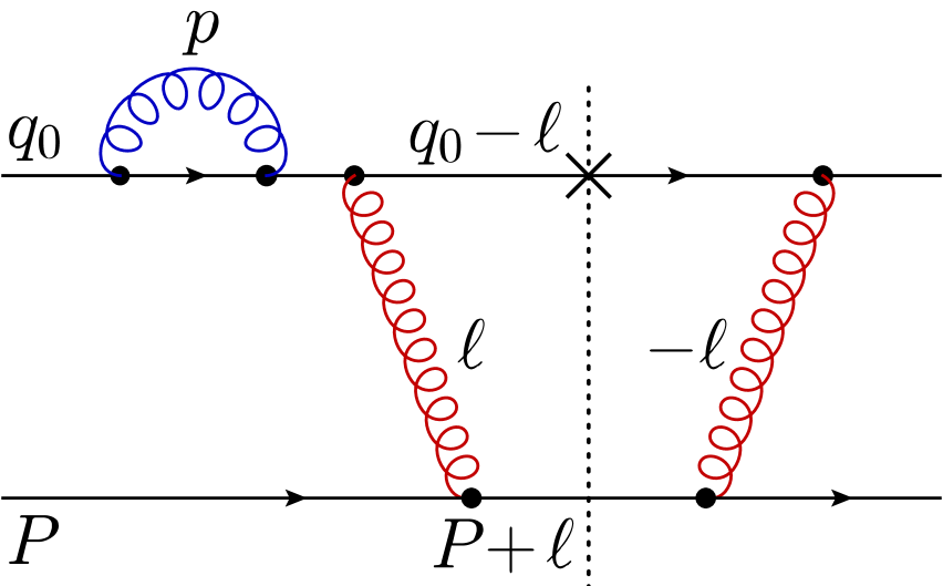
(A)

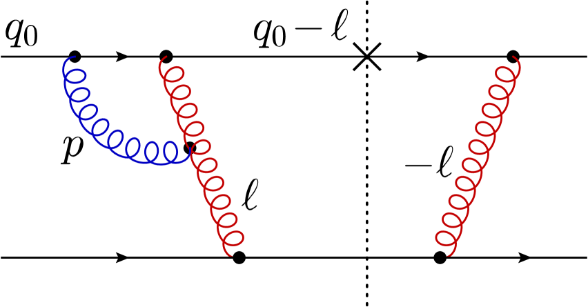
(B1)

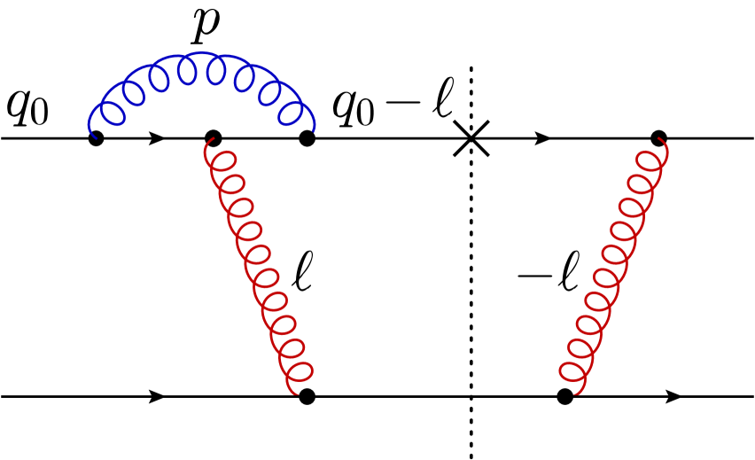
(B2)

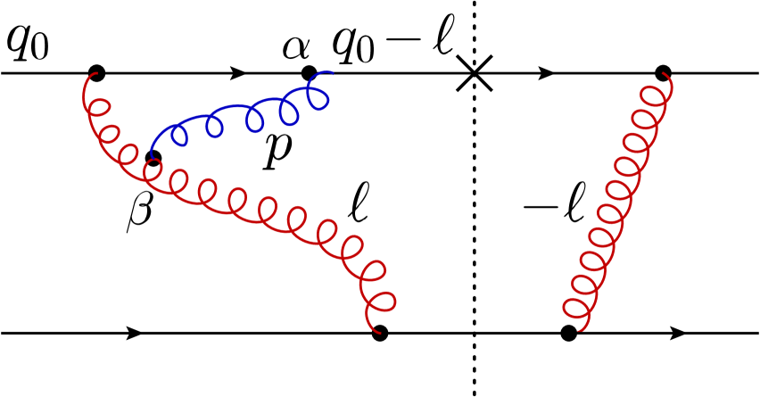
(C1)

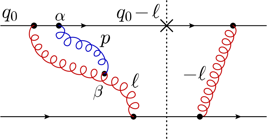
(C2)

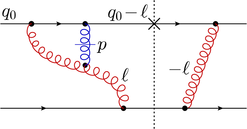
(C3)

(D)

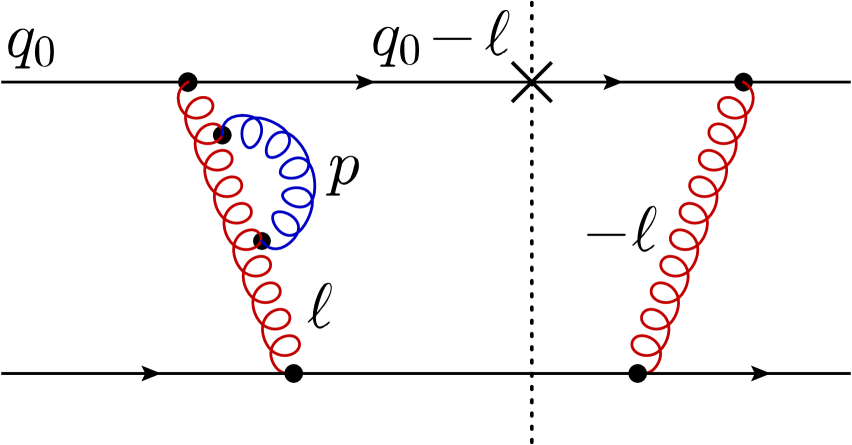
(E)

Figure 15: The virtual diagrams when $p_{\perp}\lesssim k_{\perp}$. In contrast to those in Fig. 14, the shortly lived $p$-line can be now attached to the gluon “exchange” $\ell$-line. Four-momenta are shown in the graphs and flow from the left to the right. As in the text, $q_{0}=(q_{0}^{+},0,\bm{0})$, $P=(0,P^{-},\bm{0})$, $\ell=(\ell^{+},\ell^{-},-\bm{k})$ and $p=(p^{+},p^{-},\bm{p})$, with $\ell^{-}=k_{\perp}^{2}/2\ell^{+}$ and $p^{-}=p_{\perp}^{2}/2p^{+}$. Just for C1, and for our convenience in the calculation, we let $\bm{p}\to-\bm{p}$.

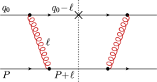
(a)

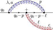
(b)

Figure 16: (a) Tree level diagram and (b) loop correction for the diagram B2 in Fig. 15. Four-momenta are shown in the graphs and flow from the left to the right.

We are not going to give a detailed calculation for all the diagrams appearing in Fig. 15, but only deal with some representative cases. Therefore, let us start by considering the diagram B2, which is decomposed in terms of the basic tree-level graph and the loop correction as shown in Fig. 16. In LCPT, we can write this loop correction as

$${\rm B2}|_{\rm loop}\to({\rm i}g)^{2}t^{a}t^{c}t^{a}\int \frac{{\rm d}^{2}\bm{p}\,{\rm d}p^{+}}{(2\pi)^{3}2p^{+}}\,\frac{1}{\frac{\bm{p}^{2}}{2p^{+}}+\frac{(\bm{q}_{0}-\bm{p})^{2}}{2(q^{+}_{0}-p^{+})}}\,\frac{1}{\frac{\bm{p}^{2}}{2p^{+}}+\frac{(\bm{q}_{0}-\bm{p}+\bm{k})^{2}}{2(q_{0}^{+}-p^{+}-\ell^{+})}+\frac{\bm{k}^{2}}{2\ell^{+}}}$$

$$\times\gamma\!\cdot\!\epsilon^{\lambda}(p)\,\gamma\!\cdot\!(q_{0}-p-\ell)\,\gamma^{+}\gamma\!\cdot\!(q_{0}-p)\,\gamma\!\cdot\!\epsilon^{\lambda}(p)\,\frac{1}{(2q_{0}^{+})^{2}},$$ (55)

where $t^{a}$ are the SU(3) generators in the fundamental representation and $\epsilon^{\lambda}(p)$ are the polarization vectors in the projectile light-cone gauge $A^{+}=0$, given by

$$\epsilon^{\lambda}(p)=\Big{(}0,\epsilon^{\lambda-}=\frac{\bm{\epsilon}^{\lambda}\!\cdot\!\bm{p}}{p^{+}},\bm{\epsilon}^{\lambda}\Big{)},$$ (56)

with $\bm{\epsilon}^{\lambda}$ two complex orthonormal two-dimensional vectors. Notice that since $p^{+}$ is very small, $\epsilon^{\lambda-}$ is the dominant component of the polarization vector. Using $\bm{q}_{0}=0$, $q_{0}^{+}\gg\ell^{+}\gg p^{+}$ and the condition in Eq. (54) which fixes $\ell^{+}$, one readily finds that the dominant term within both energy denominators and in the regime of interest (i.e. for $p_{\perp}\lesssim k_{\perp}$ and $2p^{+}/p_{\perp}^{2}\ll 1/P^{-}$) is the light-cone energy $\bm{p}^{2}/2p^{+}$ of the virtual gluon. This was to be expected since, as already said, the $p$-line is by far the one with the shortest lifetime. Regarding the inner products, we have $\gamma\cdot(q_{0}-p-\ell)\simeq\gamma\cdot(q_{0}-p)\simeq\gamma^{-}q_{0}^{+}$ and $\gamma\cdot\epsilon^{\lambda}(p)\simeq\gamma^{+}\bm{\epsilon}^{\lambda}\cdot\bm{p}/p^{+}$. Then, by using $t^{a}t^{c}t^{a}=-(C_{\rm F}-N_{\rm c}/2)t^{c}$ and putting aside a factor $t^{c}\gamma^{+}$ which is part of the tree-level graph, we eventually arrive at

$${\rm B2}|_{\rm loop}=\frac{\alpha_{s}}{\pi}\left(C_{\rm F}-N_{\rm c}/2\right)\int\frac{{\rm d}p^{+}}{p^{+}}\frac{{\rm d}p_{\perp}^{2}}{p_{\perp}^{2}}.$$ (57)

One can calculate in a similar fashion the diagrams A, B1, D and E to find

$${\rm A}|_{\rm loop}={\rm D}|_{\rm loop}=-\frac{\alpha_{s}C_{\rm F}}{2\pi}\int\frac{{\rm d}p^{+}}{p^{+}}\frac{{\rm d}p_{\perp}^{2}}{p_{\perp}^{2}}\,,\qquad{\rm B1}|_{\rm loop}=-{\rm E}|_{\rm loop}=\frac{\alpha_{s}N_{\rm c}}{2\pi}\int\frac{{\rm d}p^{+}}{p^{+}}\frac{{\rm d}p_{\perp}^{2}}{p_{\perp}^{2}}.$$ (58)

The factor $-1/2$ for diagrams A and D emerges from the calculation and it is the usual factor associated with the wavefunction renormalization. A similar argument applies to diagram E, however in that case we have put the factor 1/2 by hand, since half of the full result should be attached to the lower vertex of the $\ell$-line.

Now let us move to the C diagrams, for which it is not hard to see that they will have the same color factor $N_{\rm c}/2$ with diagram B1. We have

$${\rm C}|_{\rm loop}\to-({\rm i}g)^{2}\frac{N_{c}}{2}\int\frac{{\rm d}^{2}\bm{p}\,{\rm d}p^{+}}{(2\pi)^{3}2p^{+}}\,\frac{1}{\frac{(\bm{k}+\bm{p})^{2}}{2\ell^{+}}}\left[\frac{4n_{\alpha}n_{\beta}}{p^{+}}-\frac{\epsilon^{\lambda}_{\alpha}(p)\epsilon^{\lambda}_{\beta}(p)}{\frac{\bm{p}^{2}}{2p^{+}}+\frac{\bm{k}^{2}}{2\ell^{+}}}-\frac{\epsilon^{\lambda}_{\alpha}(p)\epsilon^{\lambda}_{\beta}(p)}{\frac{\bm{p}^{2}}{2p^{+}}+\frac{(\bm{k}+\bm{p})^{2}}{2\ell^{+}}}\right]\frac{\gamma^{\alpha}\,\gamma\!\cdot\!q_{0}\,\gamma^{+}}{2q_{0}^{+}}\,\frac{2\ell^{\beta}}{2\ell^{+}},$$ (59)

where each term in the square bracket represents the respective contribution from C1, C2 and C3. The 4-vector $n$, appearing in the instantaneous term, is such that $n\cdot\upsilon=\upsilon^{+}$ for any vector $\upsilon^{\alpha}$. In Eq. (59) we have already simplified the energy denominators (in particular we have neglected the terms suppressed by $1/q_{0}^{+}$) and kept only the terms that will contribute to the final result (notice also that in C1 we have let $\bm{p}\to-\bm{p}$ in order to combine them in an elegant way). Since $\epsilon^{\lambda-}$ is the large component of the polarization vector, we need to keep only the $--$ component of the tensor structure in the square bracket (notice that the indices here have been raised), which becomes

$$\Big{[}\cdots\Big{]}^{--}=\frac{4}{p^{+}}-\frac{\frac{\bm{p}^{2}}{(p^{+})^{2}}}{\frac{\bm{p}^{2}}{2p^{+}}+\frac{\bm{k}^{2}}{2\ell^{+}}}-\frac{\frac{\bm{p}^{2}}{(p^{+})^{2}}}{\frac{\bm{p}^{2}}{2p^{+}}+\frac{(\bm{k}+\bm{p})^{2}}{2\ell^{+}}}.$$ (60)

Here it becomes clear that we cannot make the immediate approximation to keep only the $\bm{p}^{2}/2p^{+}$ in the energy denominators (as we did for the previous class of diagrams), since the leading term cancels. It is a matter of straightforward algebra to find the dominant surviving terms:

$$\Big{[}\cdots\Big{]}^{--}\simeq\frac{4}{\bm{p}^{2}}\,\left[\frac{(\bm{k}+\bm{p})^{2}}{2\ell^{+}}+\frac{\bm{k}^{2}}{2\ell^{+}}\right].$$ (61)

Since the transverse momentum of the exchange gluon is $\bm{k}+\bm{p}$ when attached to the upper vertex and $\bm{k}$ when attached to the lower one, only the first term in Eq. (61) should be kept for our purposes, and Eq. (59) leads to

$${\rm C}|_{\rm loop}=\frac{\alpha_{s}N_{\rm c}}{2\pi}\int\frac{{\rm d}p^{+}}{p^{+}}\frac{{\rm d}p_{\perp}^{2}}{p_{\perp}^{2}}.$$ (62)

Putting Eqs. (57), (58) and (62) together, it is obvious that

$${\rm A+B+C+D+E}=0,$$ (63)

which is the aforementioned cancellation of virtual corrections in the regime under consideration. Perhaps the most intuitive way to view this result is to realize that in diagrams C, D and E the shortly-lived gluon with momentum $p$ is emitted after the ‘exchanged’ gluon. The gluon in the ‘exchange’ line has a transverse velocity $|\bm{k}+\bm{p}|/\ell^{+}\sim k_{\perp}/\ell^{+}$, so that over the small lifetime $2p^{+}/p_{\perp}^{2}$ of the $p$-fluctuation it separates from the quark $q_{0}$ only a very small distance

$$\Delta x_{\perp}\simeq\frac{k_{\perp}}{\ell^{+}}\,\frac{2p^{+}}{p_{\perp}^{2}}\sim\frac{2}{k_{\perp}}\,\frac{k_{\perp}^{2}}{2\ell^{+}}\,\frac{2p^{+}}{p_{\perp}^{2}}=\frac{2}{k_{\perp}}\,\frac{2p^{+}P^{-}}{p_{\perp}^{2}}\ll\frac{2}{k_{\perp}}.$$ (64)

To arrive at the above we have used Eq. (54) and the fact that $2p^{+}/p_{\perp}^{2}\ll 1/P^{-}$. Therefore, the system composed of the quark and the ‘exchanged’ gluon looks like a quark during the time interval defined by the emission and the reabsorption of the virtual, $p$-gluon. Indeed, one has

$$\left({\rm C+D+E}\right)|_{\rm loop}=-\frac{\alpha_{s}C_{\rm F}}{2\pi}\int\frac{{\rm d}p^{+}}{p^{+}}\frac{{\rm d}p_{\perp}^{2}}{p_{\perp}^{2}},$$ (65)

which can be associated with the quark wavefunction renormalization factor, more precisely with

$$\sqrt{Z_{2}}-1=\sqrt{1+\left(Z_{2}-1\right)}-1\simeq\frac{1}{2}\left(Z_{2}-1\right),$$ (66)

where the r.h.s. follows since $Z_{2}-1\sim\alpha_{s}\ll 1$. Similarly graph A gives another factor of $1/2(Z_{2}-1)$, while graphs B can be identified with the quark-gluon vertex renormalization factor $Z_{1}$ to order $\alpha_{s}$ :

$$({\rm B_{1}+B_{2}})|_{\rm loop}=\frac{1}{Z_{1}}-1\simeq 1-Z_{1}.$$ (67)

Therefore, it is instructive to rewrite the sum of the one-loop virtual corrections as follows

$$\left[1+\frac{1}{2}\left(Z_{2}-1\right)\right]\left[1+\left(\frac{1}{Z_{1}}-1\right)\right]\left[1+\frac{1}{2}\left(Z_{2}-1\right)\right]-1\simeq\sqrt{Z_{2}}\,\frac{1}{Z_{1}}\,\sqrt{Z_{2}}-1,$$ (68)

so that the first factor in the square bracket can be identified with $1+{\rm A|_{loop}}$, the second with $1+({\rm B_{1}+B_{2}})|_{\rm loop}$ and the last with ${\rm 1+(C+D+E)|_{loop}}$. The fact that our calculation gives $Z_{2}-1=$ $-(1/Z_{1}-1)$ at order $\alpha_{s}$, making the right hand side in Eq. (68) equal to zero, can be interpreted as the condition $Z_{1}=Z_{2}$ valid in light cone gauge. At a first glance, it may seem strange to identify our calculation with an evaluation of renormalization constants when $p_{\perp}$ is not large, however one can check that the Slavnov-Taylor-Ward identities indeed require ${\rm 2A+B}=0$, as explicitly shown above.

Appendix B Target versus projectile evolution beyond LO

The NLO expressions for the quark multiplicity in Eqs. (3.3) or (3.3) involve dipole $S$-matrices like $\mathcal{S}\big{(}\bm{q},X(x)\big{)}$, which in the main text have been assumed to follow the target evolution with decreasing $X=q^{-}/P^{-}$, from $X=X_{0}$ down to $X(x)\ll 1$. The viewpoint of target evolution was indeed more convenient at a conceptual level, for developing a physical picture and also for formulating kinematical constraints like the energy conservation (8). This is however less convenient in practice, because the high-energy evolution of a dense nucleus is not known beyond LO (i.e. beyond rcBK). Yet, as we shall now explain, this unknown target evolution can be replaced for the present purposes with the evolution of the dilute projectile, which is indeed known to the accuracy of interest.

More precisely, what is known is the NLO version of the BK equation in coordinate space Balitsky:2008zza ; Balitsky:2013fea ; Kovner:2013ona together with its ‘collinear improvement’ Beuf:2014uia ; Iancu:2015vea ; Iancu:2015joa ; Hatta:2016ujq . When adapting these equations to the problem at hand, the only subtlety refers to the proper identification of the longitudinal phase-space for the evolution of the projectile — that is, the interval in $p^{+}$ which is spanned by the evolution gluons. This identification was straightforward at LO, where the ‘plus’ and ‘minus’ rapidities can be identified with each other, as discussed in Sect. 2.3, but it is less trivial beyond LO, where the exact kinematics becomes important (recall also the discussion towards the end of Sect. 3.4).

When discussing projectile evolution in what follows, one should keep in mind that the relevant ‘projectile’ is the right-moving partonic pair made with the incoming quark and its primary gluon. The kinematics of that pair, in particular the 3-momentum $(p^{+}=xq_{0}^{+},\bm{p})$ of the primary gluon, must be considered as fixed for the purposes of the evolution — this matter only for the boundaries of the evolution phase-space. The evolution rather refers to the three dipoles $S$-matrices $\mathcal{S}(\bm{q})$, $\mathcal{S}(\bm{\ell})$, and $\mathcal{S}(\bm{k})$ which appear in Eqs. (18) and (19) — and hence implicitly in equations like (3.2) or (3.3) — and describe the scattering between the primary quark-gluon pair (the ‘projectile’) and the nuclear target (whose wavefunction is not evolving anymore, as we now work in the infinite momentum frame of the projectile). These dipoles, that we referred to as ‘daughter dipoles’ when discussing the primary emission in Sect. 3.1, will now act as parent dipoles for the high-energy evolution. That is, the ‘evolution gluons’ will be soft gluons which belong to the wavefunctions of these three dipoles and whose longitudinal momenta $p^{+}_{i}=x_{i}q_{0}^{+}$ are necessarily smaller than the corresponding momentum $p^{+}=xq_{0}^{+}$ of the primary gluon. In what follows, we shall pick one of them, say $\mathcal{S}(\bm{q})$, and study its high-energy evolution beyond LO. Previously, we have (formally) expressed the result in terms of the evolution of the target, like $\mathcal{S}\big{(}\bm{k},X(x)\big{)}$. In what follows, we would like to compute the same quantity from the evolution of the dipole $\mathcal{S}(\bm{q})$ itself, which is known beyond NLO.

Let us first recall, from the discussion in Sect. 2.3, that at LO one simply has $\mathcal{S}_{\rm\scriptscriptstyle T}\big{(}\bm{q},X(x)\big{)}=\mathcal{S}_{\rm\scriptscriptstyle P}\big{(}\bm{q},x_{g}/x\big{)}$, where we have temporarily introduced the subscripts T (‘target’) and P (‘projectile’), to make the discussion more transparent. The rapidity argument $x_{g}/x$ of $\mathcal{S}_{\rm\scriptscriptstyle P}$ can be understood as follows: the evolution variable is the longitudinal fraction $z_{i}\equiv x_{i}/x$ of a generic evolution gluon w.r.t. the parent dipole. At LO, this is bounded by $x_{g}/x<z_{i}<1$, where the lower limit comes from the kinematical limit $X(x_{i})=x_{g}/x_{i}\leq 1$. In other terms, the function $\mathcal{S}_{\rm\scriptscriptstyle P}\big{(}\bm{q},x_{g}/x\big{)}$ encodes the probability to find a gluon with longitudinal fraction $x_{g}$ within the quark-gluon projectile (see also Fig. 1).

In what follows, we shall argue that beyond LO, the above relation should be extended to

$$\mathcal{S}_{\rm\scriptscriptstyle T}\big{(}\bm{q},X(x)\big{)}\,=\,\mathcal{S}_{\rm\scriptscriptstyle P}\big{(}\bm{q},x_{\rm\scriptscriptstyle T}/x_{\rm\scriptscriptstyle P}\big{)}\,,\quad\mbox{where}\quad x_{\rm\scriptscriptstyle T}\equiv\frac{(1-x)Q_{0}^{2}}{\hat{s}}\,,\quad x_{\rm\scriptscriptstyle P}\equiv x(1-x)\mbox{min}\bigg{\{}1,\,\frac{q_{\perp}^{2}}{k_{\perp}^{2}}\bigg{\}}\,,$$ (69)

where $Q_{0}$ is the ‘infrared cutoff’ introduced by the initial condition at $x_{0}\sim 1$, e.g. the target saturation momentum at low energy (and the lowest transverse momentum scale in the problem). As before, $x_{\rm\scriptscriptstyle T}$ refers to the softest gluon in the wavefunction of the projectile which is involved in the collision, whereas $x_{\rm\scriptscriptstyle P}$ to the hardest gluon that can be emitted by the primary quark-gluon pair. The differences between $x_{\rm\scriptscriptstyle T}$ and $x_{g}$ and, respectively, between $x_{\rm\scriptscriptstyle P}$ and $x$, are consequences of time-ordering, as we shall shortly explain. It is understood that the function $\mathcal{S}_{P}$ obeys a suitable ‘beyond LO’ version of the BK equation, which includes ‘collinear improvement’ Beuf:2014uia ; Iancu:2015vea ; Iancu:2015joa ; Albacete:2015xza ; Lappi:2016fmu ; Hatta:2016ujq — that is, which includes an all-order resummation of the radiative corrections enhanced by double collinear logarithms. This equation, conveniently written as a differential equation in the plus rapidity $Y\equiv\ln(x/x_{\rm\scriptscriptstyle T})$, must be integrated from $Y_{0}\simeq 0$ (where one can use the initial condition $\mathcal{S}_{0}$ from the MV model) up to $Y_{\rm\scriptscriptstyle P}\equiv\ln({x_{\rm\scriptscriptstyle P}}/{x_{\rm\scriptscriptstyle T}})$. Full NLO accuracy can be achieved by using the NLO version of the BK equation Balitsky:2008zza amended by collinear improvement Iancu:2015vea ; Iancu:2015joa (the feasibility of such a calculation has been demonstrated in Lappi:2016fmu ).

To justify Eq. (69), consider the evolution of the original quark-gluon pair via successive emissions of soft gluons (see Fig. 17). We focus on the ‘collinear regime’ at $k_{\perp}\gg Q_{0}$, where the collinear resummations are actually needed. Then the projectile evolution looks rather similar as at LO, in the sense that it is dominated by gluon emissions which are strongly ordered in both longitudinal ($x\gg x_{1}\gg x_{2}\dots\gg x_{\rm\scriptscriptstyle T}$) and transverse ($p_{\perp}\gg p_{\perp 1}\gg p_{\perp 2}\dots\gg Q_{0}$) momenta, but which beyond LO must be also ordered in time : $\Delta x^{+}>\Delta x^{+}_{1}>\Delta x^{+}_{2}\dots>1/P^{-}$.

In the above, $x=p^{+}/q^{+}_{0}$ and $p_{\perp}=|\bm{p}|$ refer to the kinematics of the primary gluon, as before, while $x_{i}=p^{+}_{i}/q^{+}_{0}$ and $p_{\perp i}=|\bm{p}_{i}|$, with $i=1,\,2,\,\dots n$, refer to the subsequent gluons in the cascade, which are softer. The ‘lifetime’ of the $i$th generation, as given by the uncertainty principle or by the respective energy denominator, is roughly $\Delta x^{+}_{i}\simeq 2p^{+}_{i}/p_{\perp i}^{2}$. The ‘lifetime’ $\Delta x^{+}$ of the primary gluon can be similarly estimated as $\Delta x^{+}\simeq 2p^{+}/p_{\perp}^{2}$ or, more precisely (after using the complete energy denominator for the quark-gluon fluctuation),

$$\frac{1}{\Delta x^{+}}\simeq\frac{k_{\perp}^{2}}{2(1-x)q^{+}_{0}}+\frac{p_{\perp}^{2}}{2xq^{+}_{0}}\sim\frac{k_{\perp}^{2}}{2x(1-x)q^{+}_{0}}\,,$$ (70)

where in the final equality we have used $p_{\perp}\sim k_{\perp}$, in line with the arguments leading to Eq. (3.3).

Notice that, since both longitudinal ($p^{+}_{i}$) and transverse ($p_{\perp i}$) momenta are simultaneously decreasing during the evolution, the condition of time-ordering, $\Delta x^{+}_{i}>\Delta x^{+}_{i+1}$, is not automatically satisfied: the LLA includes unphysical configurations for which this condition is in fact violated. This is corrected when going beyond LO, but the respective corrections are large (since they have to ‘subtract’ for double-logarithmic regions in phase-space) and hence must be resummed to all orders. This is achieved by the ‘collinear resummations’ aforementioned Beuf:2014uia ; Iancu:2015vea ; Iancu:2015joa ; Hatta:2016ujq , which essentially amount to enforcing time-ordering within the projectile evolution.

 

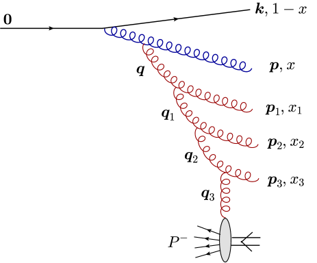
Figure 17: A sequence of emissions contributing to the evolution of the quark-gluon projectile in the collinear regime. Both longitudinal and transverse momenta are strongly ordered down the cascade. The transferred momenta $q_{\perp i}$ are relatively soft, $q_{\perp i}\ll p_{\perp i}$, hence we also have $q_{\perp}\simeq p_{\perp 1}$, $q_{\perp 1}\simeq p_{\perp 2}$, etc.

Specifically, for the first emission, the condition $\Delta x^{+}_{1}<\Delta x^{+}$ immediately implies $x_{1}\lesssim x_{\rm\scriptscriptstyle P}$ with $x_{\rm\scriptscriptstyle P}$ as defined in Eq. (69). (To obtain this, we have also used the fact that $p_{\perp 1}\simeq q_{\perp}\ll k_{\perp}$, cf. Fig. 17.) That is, the longitudinal momentum of the first gluon which counts for the evolution of $\mathcal{S}_{\rm\scriptscriptstyle P}(\bm{q})$ is not limited (from the above) by the respective momentum $p^{+}=xq_{0}^{+}$ of the primary quark, but by the generally smaller value $x_{\rm\scriptscriptstyle P}q_{0}^{+}$. Similarly, the condition that the lifetime $\Delta x^{+}_{n}$ of the last (i.e. softest) emitted gluon be larger than the longitudinal extent $1/P^{-}$ of the target, implies

$$x_{n}\,\gtrsim\,\frac{p_{\perp n}^{2}}{2q_{0}^{+}P^{-}}=(1-x)\frac{p_{\perp n}^{2}}{\hat{s}}\,>\,(1-x)\frac{Q_{0}^{2}}{\hat{s}}=x_{\rm\scriptscriptstyle T}\,,$$ (71)

where we have also used $q_{0}^{+}/Q^{+}=x_{p}/(1-x)$ for the ‘real’ terms. These considerations confirm that the longitudinal phase-space for the high-energy evolution of the quark-gluon ‘projectile’ is given by $x_{\rm\scriptscriptstyle T}<x_{i}<x_{\rm\scriptscriptstyle P}$, in agreement with Eq. (69).

Note that rapidity interval $Y_{\rm\scriptscriptstyle P}=\ln(x_{\rm\scriptscriptstyle P}/x_{\rm\scriptscriptstyle T})$ available for the evolution of the projectile is larger (when ${q_{\perp}}\gg{Q_{0}}$) than the corresponding interval $Y=\ln\big{(}{1}/{X(x)}\big{)}$ for the evolution of the target:

$$Y_{\rm\scriptscriptstyle P}=\,\ln\frac{x_{\rm\scriptscriptstyle P}}{x_{\rm\scriptscriptstyle T}}\,=\,\ln\frac{x\hat{s}}{k_{\perp}^{2}}+\ln\frac{q_{\perp}^{2}}{Q_{0}^{2}}\,=Y+\ln\frac{q_{\perp}^{2}}{Q_{0}^{2}}\,.$$ (72)

This difference is compensated by time-ordering, which effectively reduces the phase-space for the evolution of the projectile.

Appendix C NLO BK evolution and its collinear improvement

The BK equation describes the rapidity evolution of the $S$-matrix $S_{\bm{x}\bm{y}}=1-T_{\bm{x}\bm{y}}$ for the scattering of a color dipole with transverse coordinates ($\bm{x},\bm{y}$) off a hadronic target. This equation is currently known to NLO accuracy Balitsky:2008zza . Neglecting the terms suppressed in the multi-color limit $N_{\rm c}\gg 1$, one finds a closed equation for $S_{\bm{x}\bm{y}}$ which, in the spirit of Eq. (2.3), can be written in the integral form

$$\delta S_{\bm{x}\bm{y}}(x_{\rm\scriptscriptstyle T})=\, \frac{\bar{\alpha}_{s}}{2\pi}\int_{x_{\rm\scriptscriptstyle T}}^{1}\frac{{\rm d}x}{x}\int{\rm d}^{2}\bm{z}\,\frac{(\bm{x}\!-\!\bm{y})^{2}}{(\bm{x}\!-\!\bm{z})^{2}(\bm{y}\!-\!\bm{z})^{2}}\,\bigg{\{}1+\bar{\alpha}_{s}\bigg{[}\bar{b}\,\ln(\bm{x}\!-\!\bm{y})^{2}\mu^{2}-\bar{b}\,\frac{(\bm{x}\!-\!\bm{z})^{2}-(\bm{y}\!-\!\bm{z})^{2}}{(\bm{x}\!-\!\bm{y})^{2}}\ln\frac{(\bm{x}\!-\!\bm{z})^{2}}{(\bm{y}\!-\!\bm{z})^{2}}$$

$$\hskip 71.13188pt+\frac{67}{36}-\frac{\pi^{2}}{12}-\frac{5N_{\rm f}}{18N_{\rm c}}-\frac{1}{2}\ln\frac{(\bm{x}\!-\!\bm{z})^{2}}{(\bm{x}\!-\!\bm{y})^{2}}\ln\frac{(\bm{y}\!-\!\bm{z})^{2}}{(\bm{x}\!-\!\bm{y})^{2}}\bigg{]}\bigg{\}}\left[S_{\bm{x}\bm{z}}(x)S_{\bm{z}\bm{y}}(x)-S_{\bm{x}\bm{y}}(x)\right]$$

$$+\frac{\bar{\alpha}_{s}^{2}}{8\pi^{2}}\int_{x_{\rm\scriptscriptstyle T}}^{1}\frac{{\rm d}x}{x}\int\frac{{\rm d}^{2}\bm{u}\,{\rm d}^{2}\bm{z}}{(\bm{u}\!-\!\bm{z})^{4}}\bigg{\{}-2+\frac{(\bm{x}\!-\!\bm{u})^{2}(\bm{y}\!-\!\bm{z})^{2}+(\bm{x}\!-\!\bm{z})^{2}(\bm{y}\!-\!\bm{u})^{2}-4(\bm{x}\!-\!\bm{y})^{2}(\bm{u}\!-\!\bm{z})^{2}}{(\bm{x}\!-\!\bm{u})^{2}(\bm{y}\!-\!\bm{z})^{2}-(\bm{x}\!-\!\bm{z})^{2}(\bm{y}\!-\!\bm{u})^{2}}\ln\frac{(\bm{x}\!-\!\bm{u})^{2}(\bm{y}\!-\!\bm{z})^{2}}{(\bm{x}\!-\!\bm{z})^{2}(\bm{y}\!-\!\bm{u})^{2}}$$

$$\hskip 73.97733pt+\frac{(\bm{x}\!-\!\bm{y})^{2}(\bm{u}\!-\!\bm{z})^{2}}{(\bm{x}\!-\!\bm{u})^{2}(\bm{y}\!-\!\bm{z})^{2}}\left[1+\frac{(\bm{x}\!-\!\bm{y})^{2}(\bm{u}\!-\!\bm{z})^{2}}{(\bm{x}\!-\!\bm{u})^{2}(\bm{y}\!-\!\bm{z})^{2}-(\bm{x}\!-\!\bm{z})^{2}(\bm{y}\!-\!\bm{u})^{2}}\right]\ln\frac{(\bm{x}\!-\!\bm{u})^{2}(\bm{y}\!-\!\bm{z})^{2}}{(\bm{x}\!-\!\bm{z})^{2}(\bm{y}\!-\!\bm{u})^{2}}\bigg{\}}$$

$$\hskip 73.97733pt\left[S_{\bm{x}\bm{u}}(x)S_{\bm{u}\bm{z}}(x)S_{\bm{z}\bm{y}}(x)-S_{\bm{x}\bm{u}}(x)S_{\bm{u}\bm{y}}(x)\right]$$

$$+\frac{\bar{\alpha}_{s}^{2}}{8\pi^{2}}\,\frac{N_{\rm f}}{N_{\rm c}}\int_{x_{\rm\scriptscriptstyle T}}^{1}\frac{{\rm d}x}{x}\int\frac{{\rm d}^{2}\bm{u}\,{\rm d}^{2}\bm{z}}{(\bm{u}\!-\!\bm{z})^{4}}\bigg{[}2-\frac{(\bm{x}\!-\!\bm{u})^{2}(\bm{y}\!-\!\bm{z})^{2}+(\bm{x}\!-\!\bm{z})^{2}(\bm{y}\!-\!\bm{u})^{2}-(\bm{x}\!-\!\bm{y})^{2}(\bm{u}\!-\!\bm{z})^{2}}{(\bm{x}\!-\!\bm{u})^{2}(\bm{y}\!-\!\bm{z})^{2}-(\bm{x}\!-\!\bm{z})^{2}(\bm{y}\!-\!\bm{u})^{2}}\ln\frac{(\bm{x}\!-\!\bm{u})^{2}(\bm{y}\!-\!\bm{z})^{2}}{(\bm{x}\!-\!\bm{z})^{2}(\bm{y}\!-\!\bm{u})^{2}}\bigg{]}$$

$$\hskip 73.97733pt\left[S_{\bm{x}\bm{z}}(x)S_{\bm{u}\bm{y}}(x)-S_{\bm{x}\bm{u}}(x)S_{\bm{u}\bm{y}}(x)\right],$$ (73)

where $N_{\rm f}$ is the number of flavors, the coupling $\bar{\alpha}_{s}$ is evaluated at the renormalization scale $\mu$, while $\bar{\alpha}_{s}$ and $\bar{b}$ have been defined in the main text. Notice also that, for economy with respect to the notation used in Eq. (40) and afterwards, we have let $x\to x_{\rm\scriptscriptstyle T}/x$ and put the dependence on the transverse coordinates as subscripts. The $\delta$ in front $S_{\bm{x}\bm{y}}(x_{\rm\scriptscriptstyle T})$ stands for the change from the initial condition, while the quantity $\Delta S$ that we have used in the main text stands for the $\bar{\alpha}_{s}^{2}$ terms on the r.h.s. of the above equation, except for those which are proportional to $\bar{b}$.

The term with a single integration (SI) over the transverse coordinate $\bm{z}$ keeps the same structure as the LO equation, but receives a correction of order $\mathcal{O}(\bar{\alpha}_{s}^{2})$ to the kernel. In particular, it contains the running coupling corrections proportional to $\bar{b}$. The terms of order $\mathcal{O}(\bar{\alpha}_{s}^{2})$ with a double integration (DI) over the coordinates $\bm{u}$ and $\bm{z}$ arise from partonic fluctuations involving two additional partons at the time of scattering. The first of such terms is independent of $N_{\rm f}$ and clearly represents the case where both daughter partons are gluons. The $S$-matrix structure $S_{\bm{x}\bm{u}}S_{\bm{u}\bm{z}}S_{\bm{z}\bm{y}}-S_{\bm{x}\bm{u}}S_{\bm{u}\bm{y}}$ corresponds to a sequence of emissions in which the original dipole $(\bm{x},\bm{y})$ emits a gluon at $\bm{u}$ giving rise to the two dipoles $(\bm{x},\bm{u})$ and $(\bm{u},\bm{y})$, and then the dipole $(\bm{u},\bm{y})$ emits a gluon at $\bm{z}$ leading to the dipoles $(\bm{u},\bm{z})$ and $(\bm{z},\bm{y})$. The ‘real’ term $S_{\bm{x}\bm{u}}S_{\bm{u}\bm{z}}S_{\bm{z}\bm{y}}$ describes the situation where both gluons interact with the target, while the ‘virtual’ term $-S_{\bm{x}\bm{u}}S_{\bm{u}\bm{y}}$ stands for the the case where the gluon at $\bm{z}$ has been emitted and reabsorbed either before, or after, the scattering. This ‘virtual’ term ensures that the potential ‘ultraviolet’ singularity due to the $1/(\bm{u}-\bm{z})^{4}$ factor in the kernel is in fact harmless. The same discussion applies to the second DI term, proportional to $N_{\rm f}$, which represents the case that the additional partons at the time of scattering are a quark and an antiquark, and thus the number of dipoles involved in the scattering is just two.

The issue with the NLO BK equation given in (C) is that there are terms in the kernels which can get large in certain kinematic regimes, thus invalidating the strict $\bar{\alpha}_{s}$-expansion. The first class of such terms contain the corrections proportional to $\bar{b}$ in the SI term in Eq. (C), and has already been discussed in Sect. 3.4. The scale $\mu$ should be chosen in such way, that the logarithms of transverse dipole sizes proportional to $\bar{b}$ (and only those) become innocuous in any kinematic regime. It is trivial to see that both choices suggested in Sect. 3.4 will cancel any potentially large logarithmic contribution. In fact, our fac prescription, cf. Eq. (32), is by definition the one in which the sum of all terms proportional to $\bar{b}$ vanishes identically.

Now we wish to discuss NLO corrections enhanced by logarithms associated with large separations in transverse sizes (or momenta) between successive emissions. These ‘collinear’ corrections become large only in the weak-scattering regime where all the dipoles are small compared to the target saturation scale $1/Q_{s}$, so that we can linearize w.r.t. to the scattering amplitude $T$. At this level, we can drop the term proportional to $N_{\rm f}/N_{\rm c}$ in Eq. (C) since it vanishes after linearization, as one can check by using the symmetry of the kernel under the interchange $\bm{u}\leftrightarrow\bm{z}$. More precisely, we consider the strongly ordered regime

$$1/Q_{s}\gg|\bm{z}-\bm{x}|\simeq|\bm{z}-\bm{y}|\simeq|\bm{z}-\bm{u}|\gg|\bm{u}-\bm{x}|\simeq|\bm{u}-\bm{y}|\gg|\bm{x}-\bm{y}|,$$ (74)

which means that the parent dipole is the smallest one, a gluon is emitted far away at $\bm{u}$, a second one even further at $\bm{z}$, but all the possible dipole sizes remain smaller than the inverse saturation momentum. Denoting by $r$, $\bar{u}$ and $\bar{z}$ the size of the parent dipole, the size of the dipoles involving $\bm{u}$ and the size of the dipoles involving $\bm{z}$, respectively, we have $r^{2}\ll\bar{u}^{2}\ll\bar{z}^{2}$.

Inspecting the SI piece in the NLO BK equation (C), it is obvious that the term which involves the double transverse logarithm (DTL) is the dominant one in the kinematic region defined in Eq. (74). In this regime we are also allowed to write $S_{\bm{x}\bm{z}}S_{\bm{z}\bm{y}}-S_{\bm{x}\bm{y}}\simeq-T_{\bm{x}\bm{z}}-T_{\bm{z}\bm{y}}+T_{\bm{x}\bm{y}}\simeq-2T(\bar{z})$, with the second approximate equality arriving from the fact that the dipole amplitude for a small dipole is roughly proportional to the dipole size squared. Thus, the net result comes from the ‘real’ term, i.e. the one which involves the large daughter dipoles.

A single transverse logarithm (STL) is hidden in the DI term. To see that, let us isolate the kernel

$$\mathcal{M}_{{\rm\scriptscriptstyle STL}}\equiv\frac{\bar{\alpha}_{s}^{2}}{8\pi^{2}(\bm{u}\!-\!\bm{z})^{4}}\bigg{[}-2+ \,\frac{(\bm{x}\!-\!\bm{u})^{2}(\bm{y}\!-\!\bm{z})^{2}+(\bm{x}\!-\!\bm{z})^{2}(\bm{y}\!-\!\bm{u})^{2}-4(\bm{x}\!-\!\bm{y})^{2}(\bm{u}\!-\!\bm{z})^{2}}{(\bm{x}\!-\!\bm{u})^{2}(\bm{y}\!-\!\bm{z})^{2}-(\bm{x}\!-\!\bm{z})^{2}(\bm{y}\!-\!\bm{u})^{2}}$$

$$\,\times\ln\frac{(\bm{x}\!-\!\bm{u})^{2}(\bm{y}\!-\!\bm{z})^{2}}{(\bm{x}\!-\!\bm{z})^{2}(\bm{y}\!-\!\bm{u})^{2}}\bigg{]},$$ (75)

which in the collinear regime can be successively written as

$$\mathcal{M}_{{\rm\scriptscriptstyle STL}}\simeq \,\frac{\bar{\alpha}_{s}^{2}}{8\pi^{2}\bar{z}^{4}}\bigg{[}-2+\frac{2\bar{u}^{2}-2\bar{u}r\cos\phi-3r^{2}}{r^{2}-2\bar{u}r\cos\phi}\ln\left(1+\frac{r^{2}-2\bar{u}r\cos\phi}{\bar{u}^{2}}\right)\bigg{]}$$

$$\simeq \,-\frac{\bar{\alpha}_{s}^{2}}{\pi^{2}}\,\frac{6-\cos^{2}\phi}{12}\,\frac{r^{2}}{\bar{u}^{2}\bar{z}^{4}}\to-\frac{11\bar{\alpha}_{s}^{2}}{24\pi^{2}}\,\frac{r^{2}}{\bar{u}^{2}\bar{z}^{4}},$$ (76)

where $\phi$ is the angle between $\bm{r}$ and any of the two dipoles involving $\bm{u}$. To arrive at (C), we first set all dipole sizes which include $\bm{z}$ equal to each other, since any subleading term would be highly suppressed by inverse powers of $\bar{z}$. This simplifies significantly the expansion in the regime of interest, since the only $z$ dependence left is the one explicit in the prefactor. Then we have taken the limit $r\ll\bar{u}$ and finally we have performed an average over the angle $\phi$ between the parent dipole and those involving $\bm{u}$. As evident in Eq. (C), the would-be leading term of order $1/\bar{z}^{4}$ has cancelled and the first non-vanishing term is suppressed by the power factor $r^{2}/\bar{u}^{2}$. Now by linearizing the $S$-matrices multiplying $\mathcal{M}_{{\rm\scriptscriptstyle STL}}$ and realizing, as in the DTL case, that the ‘real’ term dominates, we can approximate $S_{\bm{x}\bm{u}}S_{\bm{u}\bm{z}}S_{\bm{z}\bm{y}}-S_{\bm{x}\bm{u}}S_{\bm{u}\bm{y}}\simeq-T_{\bm{u}\bm{z}}-T_{\bm{z}\bm{y}}+T_{\bm{u}\bm{y}}\simeq-2T(\bar{z})$. Since this is independent of the intermediate dipole size $\bar{u}$, the integration over the latter, within the range limited by $r$ and $\bar{z}$, leads to the anticipated STL.

Thus, putting together the LO term and the two NLO ones enhanced by the STL and the DTL, one finds that the NLO BK equation in the collinear regime (74) reduces to

$$\delta T(r;x_{\rm\scriptscriptstyle T})=\bar{\alpha}_{s}\int_{x_{\rm\scriptscriptstyle T}}^{1}\frac{{\rm d}x}{x}\int_{r^{2}}^{1/Q_{s}^{2}}{\rm d}\bar{z}^{2}\,\frac{r^{2}}{\bar{z}^{4}}\left(1-\frac{1}{2}\,\bar{\alpha}_{s}\ln^{2}\frac{\bar{z}^{2}}{r^{2}}-\frac{11}{12}\,\bar{\alpha}_{s}\ln\frac{\bar{z}^{2}}{r^{2}}\right)T(\bar{z};x).$$ (77)

Clearly, for sufficiently large daughter dipoles, the NLO contributions are enhanced by large transverse logarithms and become comparable to, or larger than, the LO one. Then, the present perturbative expansion of the kernel, which is of fixed order in $\bar{\alpha}_{s}$, cannot be trusted anymore. Eventually this problematic behavior is transmitted to the solution of equations like (77) and (C) which becomes unstable, as indeed seen in Avsar:2011ds ; Lappi:2015fma ; Iancu:2015vea .

Therefore, in order to have a meaningful evolution equation, we need to identify the physical origin of the large transverse logarithms and subsequently resum them to all orders in the coupling $\bar{\alpha}_{s}$. It should be obvious by now, that such higher order terms become more important than the pure $\bar{\alpha}_{s}^{2}$ NLO terms (that is, the $\mathcal{O}(\bar{\alpha}_{s}^{2})$ corrections not enhanced by any transverse logarithm), so that the latter will be discarded in what follows. This is the approach taken in Iancu:2015vea ; Iancu:2015joa leading to the collinearly improved BK evolution equation which admits a stable solution. Before giving this equation, we shall first write its collinear limit, i.e. we shall first resum the kernel appearing in Eq. (77).

The origin of the DTLs is in the kinematics Beuf:2014uia ; Iancu:2015vea . Our main observation in Iancu:2015vea was that these large corrections arise from LCPT Feynman graphs in which the successive gluon emissions are not only strongly ordered in both longitudinal momenta and transverse momenta (or ‘dipole sizes’), but are also ordered in lifetimes (or, equivalently, in light-cone energies Beuf:2014uia ). The all-order resummation of the double collinear logarithms $[\bar{\alpha}_{s}\ln^{2}(\bar{z}^{2}/r^{2})]^{n}$, with $n=1,2,3,\dots$, eventually leads to a modification of the kernel by a multiplicative factor given in terms of the Bessel function ${\rm J}_{1}$ (see below).

The STLs find their origin in the DGLAP dynamics Iancu:2015joa . Since each power of $\bar{\alpha}_{s}$ is accompanied by a collinear logarithm, it is intuitively clear that such terms must represent DGLAP corrections to the BFKL dynamics. This is further confirmed by the fact that the coefficient $-11/12$ in front of the single logarithm in Eq. (77) can be recognized as the second-order term in the small-$\omega$ expansion of the largest eigenvalue $\mathcal{P}(\omega)$ of the DGLAP anomalous dimension matrix in the large-$N_{\rm c}$ limit, more precisely

$$\mathcal{P}(\omega)\simeq\int_{0}^{1}{\rm d}z\,z^{\omega}\left[P_{\rm GG}(z)+\frac{C_{\rm F}}{N_{\rm c}}\,P_{\rm qG}(z)\right]=\frac{1}{\omega}-A_{1}+\mathcal{O}\left(\omega\right)\quad\mbox{with}\quad A_{1}=\frac{11}{12}+\frac{N_{\rm f}}{6N_{\rm c}^{3}},$$ (78)

where the second term of $A_{1}$ can be dropped when working in the large-$N_{\rm c}$ limit. Like the factor $1/\omega$ generates a small-$x$ gluon, the piece $-A_{1}$ corresponds to the most dominant sub-leading gluon emission (the term linear in $\omega$ would correspond to the next-to-most dominant one and so on). It is not hard to follow the combinatorics for an arbitrary number of such gluon emissions associated with $A_{1}$, and one finds that the resummation of these $[\bar{\alpha}_{s}\ln(\bar{z}^{2}/r^{2})]^{n}$ terms leads to the exponentiation of the NLO correction. Of course this is only a partial resummation of STLs, but it is well-defined and in the spirit of the $\omega$-expansion introduced and developed in Salam:1998tj ; Ciafaloni:1999yw ; Ciafaloni:2003rd . Higher orders in $\omega$ would be related to next-to-most dominant gluons and beyond, and the corresponding STLs would start at higher orders in perturbation theory (NNLO or higher).

Putting together the two types of resummation, one finds that the collinear kernel in Eq. (77) should be replaced by Iancu:2015vea ; Iancu:2015joa

$$\frac{r^{2}}{\bar{z}^{4}}\,\,\frac{{\rm J}_{1}\Big{(}2\sqrt{\bar{\alpha}_{s}\ln^{2}(\bar{z}^{2}/r^{2})}\Big{)}}{\sqrt{\bar{\alpha}_{s}\ln^{2}(\bar{z}^{2}/r^{2})}}\,\left(\frac{r^{2}}{\bar{z}^{2}}\right)^{\bar{\alpha}_{s}A_{1}}.$$ (79)

The last step in our construction consists of matching the above kernel with the LO BFKL/BK one in a consistent way and reinserting the virtual and non-linear terms in the respective evolution equation. Then one arrives at the local equation

$$\delta S_{\bm{x}\bm{y}}(x_{\rm\scriptscriptstyle T})=\frac{\bar{\alpha}_{s}}{2\pi}\int_{x_{\rm\scriptscriptstyle T}}^{1}\frac{{\rm d}x}{x}\int{\rm d}^{2}\bm{z}\,\frac{(\bm{x}-\bm{y})^{2}}{(\bm{x}-\bm{z})^{2}(\bm{y}-\bm{z})^{2}}\,\mathcal{K}_{\rm DLA}\mathcal{K}_{\rm SL}\left[S_{\bm{x}\bm{z}}(x)S_{\bm{z}\bm{y}}(x)-S_{\bm{x}\bm{y}}(x)\right],$$ (80)

where the precise form of the kernels $\mathcal{K}_{\rm DLA}$ and $\mathcal{K}_{\rm SL}$ has been given in Eqs. (41) and (42).

References

- (1) G. A. Chirilli, B.-W. Xiao, and F. Yuan, “One-loop Factorization for Inclusive Hadron Production in Collisions in the Saturation Formalism,” Phys. Rev. Lett. 108 (2012) 122301, arXiv:1112.1061 [hep-ph].
- (2) G. A. Chirilli, B.-W. Xiao, and F. Yuan, “Inclusive Hadron Productions in pA Collisions,” Phys. Rev. D86 (2012) 054005, arXiv:1203.6139 [hep-ph].
- (3) Y. V. Kovchegov and A. H. Mueller, “Gluon production in current nucleus and nucleon - nucleus collisions in a quasiclassical approximation,” Nucl.Phys. B529 (1998) 451–479, arXiv:hep-ph/9802440 [hep-ph].
- (4) Y. V. Kovchegov and K. Tuchin, “Inclusive gluon production in DIS at high parton density,” Phys.Rev. D65 (2002) 074026, arXiv:hep-ph/0111362 [hep-ph].
- (5) A. Dumitru and J. Jalilian-Marian, “Forward quark jets from protons shattering the colored glass,” Phys. Rev. Lett. 89 (2002) 022301, arXiv:hep-ph/0204028 [hep-ph].
- (6) J. L. Albacete, N. Armesto, A. Kovner, C. A. Salgado, and U. A. Wiedemann, “Energy dependence of the Cronin effect from nonlinear QCD evolution,” Phys.Rev.Lett. 92 (2004) 082001, arXiv:hep-ph/0307179 [hep-ph].
- (7) D. Kharzeev, Y. V. Kovchegov, and K. Tuchin, “Cronin effect and high p(T) suppression in pA collisions,” Phys.Rev. D68 (2003) 094013, arXiv:hep-ph/0307037 [hep-ph].
- (8) E. Iancu, K. Itakura, and D. Triantafyllopoulos, “Cronin effect and high p-perpendicular suppression in the nuclear gluon distribution at small x,” Nucl.Phys. A742 (2004) 182–252, arXiv:hep-ph/0403103 [hep-ph].
- (9) J. P. Blaizot, F. Gelis, and R. Venugopalan, “High-energy pA collisions in the color glass condensate approach. 1. Gluon production and the Cronin effect,” Nucl.Phys. A743 (2004) 13–56, arXiv:hep-ph/0402256 [hep-ph].
- (10) J. P. Blaizot, F. Gelis, and R. Venugopalan, “High energy p A collisions in the color glass condensate approach. II: Quark production,” Nucl. Phys. A743 (2004) 57–91, arXiv:hep-ph/0402257.
- (11) A. Dumitru, A. Hayashigaki, and J. Jalilian-Marian, “The Color glass condensate and hadron production in the forward region,” Nucl. Phys. A765 (2006) 464–482, arXiv:hep-ph/0506308 [hep-ph].
- (12) J. L. Albacete and C. Marquet, “Single Inclusive Hadron Production at RHIC and the LHC from the Color Glass Condensate,” Phys.Lett. B687 (2010) 174–179, arXiv:1001.1378 [hep-ph].
- (13) P. Tribedy and R. Venugopalan, “QCD saturation at the LHC: comparisons of models to p+p and A+A data and predictions for p+Pb collisions,” Phys.Lett. B710 (2012) 125–133, arXiv:1112.2445 [hep-ph].
- (14) A. H. Rezaeian, “CGC predictions for p+A collisions at the LHC and signature of QCD saturation,” Phys.Lett. B718 (2013) 1058–1069, arXiv:1210.2385 [hep-ph].
- (15) T. Lappi and H. Mäntysaari, “Single inclusive particle production at high energy from HERA data to proton-nucleus collisions,” Phys.Rev. D88 (2013) 114020, arXiv:1309.6963 [hep-ph].
- (16) R. K. Ellis, W. J. Stirling, and B. R. Webber, QCD and collider physics, Camb. Monogr. Part. Phys. Nucl. Phys. Cosmol., vol. 8. Cambridge University Press, 1996.
- (17) E. Iancu, A. Leonidov, and L. McLerran, “The Color glass condensate: An Introduction,” arXiv:hep-ph/0202270 [hep-ph].
- (18) E. Iancu and R. Venugopalan, “The color glass condensate and high energy scattering in QCD,” arXiv:hep-ph/0303204.
- (19) F. Gelis, E. Iancu, J. Jalilian-Marian, and R. Venugopalan, “The Color Glass Condensate,” Ann.Rev.Nucl.Part.Sci. 60 (2010) 463–489, arXiv:1002.0333 [hep-ph].
- (20) Y. V. Kovchegov and E. Levin, Quantum chromodynamics at high energy. Cambridge University Press, 2012.
- (21) S. Catani, M. Ciafaloni, and F. Hautmann, “High-energy factorization and small x heavy flavor production,” Nucl. Phys. B366 (1991) 135–188.
- (22) S. Catani and F. Hautmann, “High-energy factorization and small x deep inelastic scattering beyond leading order,” Nucl. Phys. B427 (1994) 475–524, arXiv:hep-ph/9405388 [hep-ph].
- (23) I. Balitsky, “Operator expansion for high-energy scattering,” Nucl. Phys. B463 (1996) 99–160, arXiv:hep-ph/9509348.
- (24) J. Jalilian-Marian, A. Kovner, A. Leonidov, and H. Weigert, “The BFKL equation from the Wilson renormalization group,” Nucl. Phys. B504 (1997) 415–431, arXiv:hep-ph/9701284.
- (25) J. Jalilian-Marian, A. Kovner, A. Leonidov, and H. Weigert, “The Wilson renormalization group for low x physics: Towards the high density regime,” Phys.Rev. D59 (1998) 014014, arXiv:hep-ph/9706377 [hep-ph].
- (26) A. Kovner, J. G. Milhano, and H. Weigert, “Relating different approaches to nonlinear QCD evolution at finite gluon density,” Phys. Rev. D62 (2000) 114005, arXiv:hep-ph/0004014.
- (27) E. Iancu, A. Leonidov, and L. D. McLerran, “Nonlinear gluon evolution in the color glass condensate. I,” Nucl. Phys. A692 (2001) 583–645, arXiv:hep-ph/0011241.
- (28) E. Iancu, A. Leonidov, and L. D. McLerran, “The renormalization group equation for the color glass condensate,” Phys. Lett. B510 (2001) 133–144, arXiv:hep-ph/0102009.
- (29) E. Ferreiro, E. Iancu, A. Leonidov, and L. McLerran, “Nonlinear gluon evolution in the color glass condensate. II,” Nucl. Phys. A703 (2002) 489–538, arXiv:hep-ph/0109115.
- (30) Y. V. Kovchegov, “Small-x F2 structure function of a nucleus including multiple pomeron exchanges,” Phys. Rev. D60 (1999) 034008, arXiv:hep-ph/9901281.
- (31) A. H. Mueller and S. Munier, “-broadening and production processes versus dipole/quadrupole amplitudes at next-to-leading order,” Nucl. Phys. A893 (2012) 43–86, arXiv:1206.1333 [hep-ph].
- (32) I. Balitsky and G. A. Chirilli, “Next-to-leading order evolution of color dipoles,” Phys.Rev. D77 (2008) 014019, arXiv:0710.4330 [hep-ph].
- (33) I. Balitsky and G. A. Chirilli, “Rapidity evolution of Wilson lines at the next-to-leading order,” Phys.Rev. D88 (2013) 111501, arXiv:1309.7644 [hep-ph].
- (34) A. Kovner, M. Lublinsky, and Y. Mulian, “Jalilian-Marian, Iancu, McLerran, Weigert, Leonidov, Kovner evolution at next to leading order,” Phys.Rev. D89 (2014) no. 6, 061704, arXiv:1310.0378 [hep-ph].
- (35) E. Avsar, A. Stasto, D. Triantafyllopoulos, and D. Zaslavsky, “Next-to-leading and resummed BFKL evolution with saturation boundary,” JHEP 1110 (2011) 138, arXiv:1107.1252 [hep-ph].
- (36) T. Lappi and H. Mäntysaari, “Direct numerical solution of the coordinate space Balitsky-Kovchegov equation at next to leading order,” Phys.Rev. D91 (2015) no. 7, 074016, arXiv:1502.02400 [hep-ph].
- (37) E. Iancu, J. Madrigal, A. Mueller, G. Soyez, and D. Triantafyllopoulos, “Resumming double logarithms in the QCD evolution of color dipoles,” Phys.Lett. B744 (2015) 293–302, arXiv:1502.05642 [hep-ph].
- (38) J. Kwiecinski, A. D. Martin, and A. Stasto, “A Unified BFKL and GLAP description of F2 data,” Phys.Rev. D56 (1997) 3991–4006, arXiv:hep-ph/9703445 [hep-ph].
- (39) G. Salam, “A Resummation of large subleading corrections at small x,” JHEP 9807 (1998) 019, arXiv:hep-ph/9806482 [hep-ph].
- (40) M. Ciafaloni, D. Colferai, and G. Salam, “Renormalization group improved small x equation,” Phys.Rev. D60 (1999) 114036, arXiv:hep-ph/9905566 [hep-ph].
- (41) G. Altarelli, R. D. Ball, and S. Forte, “Resummation of singlet parton evolution at small x,” Nucl.Phys. B575 (2000) 313–329, arXiv:hep-ph/9911273 [hep-ph].
- (42) M. Ciafaloni, D. Colferai, G. Salam, and A. Stasto, “Renormalization group improved small x Green’s function,” Phys.Rev. D68 (2003) 114003, arXiv:hep-ph/0307188 [hep-ph].
- (43) A. Sabio Vera, “An ’All-poles’ approximation to collinear resummations in the Regge limit of perturbative QCD,” Nucl.Phys. B722 (2005) 65–80, arXiv:hep-ph/0505128 [hep-ph].
- (44) G. Beuf, “Improving the kinematics for low-x QCD evolution equations in coordinate space,” Phys.Rev. D89 (2014) 074039, arXiv:1401.0313 [hep-ph].
- (45) E. Iancu, J. D. Madrigal, A. H. Mueller, G. Soyez, and D. N. Triantafyllopoulos, “Collinearly-improved BK evolution meets the HERA data,” Phys. Lett. B750 (2015) 643–652, arXiv:1507.03651 [hep-ph].
- (46) Y. Hatta and E. Iancu, “Collinearly improved JIMWLK evolution in Langevin form,” JHEP 08 (2016) 083, arXiv:1606.03269 [hep-ph].
- (47) J. L. Albacete, “Resummation of double collinear logs in BK evolution versus HERA data,” arXiv:1507.07120 [hep-ph].
- (48) T. Lappi and H. Mäntysaari, “Next-to-leading order Balitsky-Kovchegov equation with resummation,” Phys. Rev. D93 (2016) no. 9, 094004, arXiv:1601.06598 [hep-ph].
- (49) T. Altinoluk and A. Kovner, “Particle Production at High Energy and Large Transverse Momentum - ’The Hybrid Formalism’ Revisited,” Phys. Rev. D83 (2011) 105004, arXiv:1102.5327 [hep-ph].
- (50) T. Altinoluk, N. Armesto, G. Beuf, A. Kovner, and M. Lublinsky, “Single-inclusive particle production in proton-nucleus collisions at next-to-leading order in the hybrid formalism,” Phys. Rev. D91 (2015) no. 9, 094016, arXiv:1411.2869 [hep-ph].
- (51) A. M. Stasto, B.-W. Xiao, and D. Zaslavsky, “Towards the Test of Saturation Physics Beyond Leading Logarithm,” Phys. Rev. Lett. 112 (2014) no. 1, 012302, arXiv:1307.4057 [hep-ph].
- (52) D. Yu. Ivanov and A. Papa, “Inclusive production of a pair of hadrons separated by a large interval of rapidity in proton collisions,” JHEP 07 (2012) 045, arXiv:1205.6068 [hep-ph].
- (53) A. M. Staśto, B.-W. Xiao, F. Yuan, and D. Zaslavsky, “Matching collinear and small factorization calculations for inclusive hadron production in collisions,” Phys. Rev. D90 (2014) no. 1, 014047, arXiv:1405.6311 [hep-ph].
- (54) Z.-B. Kang, I. Vitev, and H. Xing, “Next-to-leading order forward hadron production in the small- regime: rapidity factorization,” Phys. Rev. Lett. 113 (2014) 062002, arXiv:1403.5221 [hep-ph].
- (55) B.-W. Xiao and F. Yuan, “Comment on ”Next-to-leading order forward hadron production in the small-x regime: rapidity factorization” arXiv:1403.5221 by Kang et al,” arXiv:1407.6314 [hep-ph].
- (56) B. Ducloué, T. Lappi, and Y. Zhu, “Single inclusive forward hadron production at next-to-leading order,” Phys. Rev. D93 (2016) no. 11, 114016, arXiv:1604.00225 [hep-ph].
- (57) K. Watanabe, B.-W. Xiao, F. Yuan, and D. Zaslavsky, “Implementing the exact kinematical constraint in the saturation formalism,” Phys. Rev. D92 (2015) no. 3, 034026, arXiv:1505.05183 [hep-ph].
- (58) A. M. Stasto and D. Zaslavsky, “Saturation in inclusive production beyond leading logarithm accuracy,” arXiv:1608.02285 [hep-ph].
- (59) A. M. Stasto, K. J. Golec-Biernat, and J. Kwiecinski, “Geometric scaling for the total gamma* p cross-section in the low x region,” Phys. Rev. Lett. 86 (2001) 596–599, arXiv:hep-ph/0007192.
- (60) E. Iancu, K. Itakura, and L. McLerran, “Geometric scaling above the saturation scale,” Nucl. Phys. A708 (2002) 327–352, arXiv:hep-ph/0203137.
- (61) A. Mueller and D. Triantafyllopoulos, “The Energy dependence of the saturation momentum,” Nucl.Phys. B640 (2002) 331–350, arXiv:hep-ph/0205167 [hep-ph].
- (62) S. Munier and R. B. Peschanski, “Geometric scaling as traveling waves,” Phys. Rev. Lett. 91 (2003) 232001, arXiv:hep-ph/0309177.
- (63) C. Marquet, “Forward inclusive dijet production and azimuthal correlations in pA collisions,” Nucl. Phys. A796 (2007) 41–60, arXiv:0708.0231 [hep-ph].
- (64) J. L. Albacete and C. Marquet, “Azimuthal correlations of forward di-hadrons in d+Au collisions at RHIC in the Color Glass Condensate,” Phys. Rev. Lett. 105 (2010) 162301, arXiv:1005.4065 [hep-ph].
- (65) F. Dominguez, C. Marquet, B.-W. Xiao, and F. Yuan, “Universality of Unintegrated Gluon Distributions at small x,” Phys. Rev. D83 (2011) 105005, arXiv:1101.0715 [hep-ph].
- (66) E. Iancu and J. Laidet, “Gluon splitting in a shockwave,” Nucl.Phys. A916 (2013) 48–78, arXiv:1305.5926 [hep-ph].
- (67) D. Zaslavsky, Probing Hadron Structure in Proton-Nucleus Collisions. PhD thesis, Penn State U., 2014. arXiv:1409.8259 [hep-ph]. https://inspirehep.net/record/1319344/files/arXiv:1409.8259.pdf.
- (68) Y. V. Kovchegov and H. Weigert, “Quark loop contribution to BFKL evolution: Running coupling and leading-N(f) NLO intercept,” Nucl.Phys. A789 (2007) 260–284, arXiv:hep-ph/0612071 [hep-ph].
- (69) Y. V. Kovchegov and H. Weigert, “Triumvirate of Running Couplings in Small-x Evolution,” Nucl.Phys. A784 (2007) 188–226, arXiv:hep-ph/0609090 [hep-ph].
- (70) I. Balitsky, “Quark contribution to the small-x evolution of color dipole,” Phys.Rev. D75 (2007) 014001, arXiv:hep-ph/0609105 [hep-ph].
- (71) L. D. McLerran and R. Venugopalan, “Computing quark and gluon distribution functions for very large nuclei,” Phys. Rev. D49 (1994) 2233–2241, arXiv:hep-ph/9309289.
- (72) L. D. McLerran and R. Venugopalan, “Gluon distribution functions for very large nuclei at small transverse momentum,” Phys. Rev. D49 (1994) 3352–3355, arXiv:hep-ph/9311205.
- (73) J. L. Albacete, N. Armesto, J. G. Milhano, P. Quiroga-Arias, and C. A. Salgado, “AAMQS: A non-linear QCD analysis of new HERA data at small-x including heavy quarks,” Eur.Phys.J. C71 (2011) 1705, arXiv:1012.4408 [hep-ph].
- (74) J. L. Albacete and Y. V. Kovchegov, “Solving high energy evolution equation including running coupling corrections,” Phys.Rev. D75 (2007) 125021, arXiv:0704.0612 [hep-ph].
- (75) J. L. Albacete and C. Marquet, “Gluon saturation and initial conditions for relativistic heavy ion collisions,” Prog.Part.Nucl.Phys. 76 (2014) 1–42, arXiv:1401.4866 [hep-ph].
- (76) K. J. Golec-Biernat and M. Wusthoff, “Saturation effects in deep inelastic scattering at low and its implications on diffraction,” Phys. Rev. D59 (1998) 014017, arXiv:hep-ph/9807513.
- (77) I. Balitsky and G. A. Chirilli, “Photon impact factor in the next-to-leading order,” Phys. Rev. D83 (2011) 031502, arXiv:1009.4729 [hep-ph].
- (78) G. Beuf, “NLO corrections for the dipole factorization of DIS structure functions at low x,” Phys. Rev. D85 (2012) 034039, arXiv:1112.4501 [hep-ph].
- (79) I. Balitsky and G. A. Chirilli, “Photon impact factor and -factorization for DIS in the next-to-leading order,” Phys. Rev. D87 (2013) no. 1, 014013, arXiv:1207.3844 [hep-ph].
- (80) G. Beuf, “Dipole factorization for DIS at NLO I: Loop correction to the photon to quark-antiquark light-front wave-functions,” arXiv:1606.00777 [hep-ph].