Controlled delocalization of electronic states in a multi-strand quasiperiodic lattice

Abstract

Finite strips, composed of a periodic stacking of infinite quasiperiodic Fibonacci chains, have been investigated in terms of their electronic properties. The system is described by a tight binding Hamiltonian. The eigenvalue spectrum of such a multi-strand quasiperiodic network is found to be sensitive on the mutual values of the intra-strand and inter-strand tunnel hoppings, whose distribution displays a unique three-subband self-similar pattern in a parameter subspace. In addition, it is observed that special numerical correlations between the nearest and the next-nearest neighbor hopping integrals can render a substantial part of the energy spectrum absolutely continuous. Extended, Bloch like functions populate the above continuous zones, signalling a complete delocalization of single particle states even in such a non-translationally invariant system, and more importantly, a phenomenon that can be engineered by tuning the relative strengths of the hopping parameters. A commutation relation between the potential and the hopping matrices enables us to work out the precise correlation which helps to engineer the extended eigenfunctions and determine the band positions at will.

I Introduction

Recent years have witnessed several interesting variations of the classic case of Anderson localization  anderson ; kramer ; abrahams of electronic eigenfunctions in disordered systems. Localization of single particle eigenstates in the presence of disorder is otherwise, an ubiquitous phenomenon, extending its realm well beyond the ‘electronic’ scenario, to the arena of plasmonic christ ; ruting , phononic vasseur or polaronic excitations barinov , as well as in the field of photonics yablo ; john . The last example has gained momentum and aroused interest recently after the development of the idea of light localization using path-entangled photons gilead and the tailoring of partially coherent light svozil . The variants of the phenomenon, beginning with the concept of geometrically correlated disorder in the distribution of the potentials, the so called random dimer model (RDM) dunlap , or in the overlap integrals in a tight binding description  zhang1 , and moving over to the engineering of continuous bands of extended Bloch-like functions  sil ; rudo6 ; arunava1 ; arunava2 ; arunava3 in quasi one dimensional disordered or quasiperiodic systems, thus offer exciting physics and the prospects of designing novel devices.

In this communication we explore the possibility of engineering continuous bands of extended, Bloch like single particle states in multi-strand ladder networks, which on the whole, do not possess any translational invariance. The mesh has a finite width in the $y$-direction, but extending to infinity along the $x$-axis. Though the problem we address is valid with respect to any kind of disordered lattices, we have specifically opted to discuss a quasiperiodic network for which an exact analytical attack is possible. We work here with a mesh formed by infinitely long quasiperiodic Fibonacci chains kohmoto , grown along the $x$-direction and which are then stacked periodically in the transverse $y$-direction. This is illustrated in Fig. 1. The methodology is easily extendable to randomly disordered system of arbitrary width.

It should be appreciated that the typical correlated clusters of atomic sites, causing a local resonance

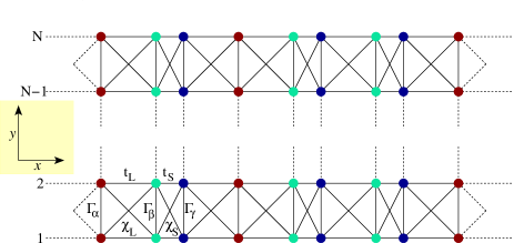
Figure 1: (Color online) An $N$-strand Fibonacci ladder made up by stacking identical Fibonacci lattices, infinitely long in the $x$-direction. The three kinds of vertices, viz., $\alpha$, $\beta$ and $\gamma$ are depicted by three different colors red, cyan and blue respectively. The second neighbor hoppings $\chi_{L}$ and $\chi_{S}$ are marked distinctly.

such as in the case of the RDM dunlap is absent here, and the spectral properties are solely controlled by the interplay of quasiperiodic order along the horizontal direction, and the translational invariance (as the system grows in the $y$-direction) in the transverse direction. Working out a condition for resonance or creation of bands of eigenvalues populated by extended Bloch-like states only in such quasi one dimensional systems thus turns out to be non-trivial. The ‘deterministic’ growth rule of a Fibonacci chain kohmoto allows for an analytical attack on the problem. We take advantage of that, obtain the exact mathematical criteria for generating absolutely continuous bands of extended single particle states, and substantiate our findings by numerically evaluating the density of states in several cases using a real space renormalization group (RSRG) decimation method.

In addition to this, we examine the effect of a line defect in the form of a linear

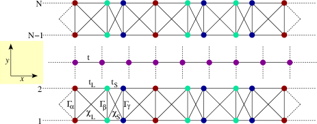
Figure 2: (Color online) An $N$-strand Fibonacci strip with an embedded periodic chain of atoms (magenta colored). All the atomic sites in the defect chain have the same on-site potential $\epsilon$ and hopping $t$.

periodic chain in the bulk of a Fibonacci stack, such as shown in Fig. 2. The system can be treated in the same mathematical footing as the previous one, and gives us a flavor of what influence can a single line defect have on the overall energy spectrum of such a quasi-periodic stack.

The backbone of our analytical attempt is an exact mapping of a coupled, quasi-one dimensional multi-strand ladder network into a set of totally decoupled linear chains describing the quantum mechanics of a class of pseudoparticles. Such an exact mapping has previously been described in the literature in the context of de-localization of single particle states in a ladder-like geometry sil ; rudo6 modelling a DNA-like double chain sil or a quasi-two dimensional mesh with correlated disorder rudo6 .

We find interesting results. For an $N$-strand Fibonacci mesh, it is possible to generate absolutely continuous subbands of eigenfunctions by introducing appropriate correlation between the numerical values of the parameters of the Hamiltonian. For an $N$ strand ladder with $N$ being an odd number, there can be just one continuous subband populated by extended states only, at a time. There can be $N-1$ different choices for this of course, each choice requiring a different correlation between the values of the on-site potentials and the nearest and next nearest neighbor hopping integrals. For even values of $N$, there can be $N$ such different conditions. The spectrum, in all the cases, loses the natural three-subband structure of a linear Fibonacci lattice kohmoto . The inter-strand coupling plays an important role. We have examined the correlation between the intra-strand ($t_{S}$) and inter-strand ($\Gamma$) hopping integrals. The distribution of the allowed combinations of these two displays an interesting three subband, self-similar pattern in the $(t_{S},\Gamma)$ subspace.

In the latter part of the work we show that the incorporation of a linear periodic chain of atoms in the bulk of such a quasiperiodic mesh has remarkable influence on the gross spectral behavior. For weak to moderate coupling this minimal heterogeneity introduced in the form of such single line defect generates regions of absolutely continuous bands. The wave functions populating such regions are found to be of extended character, as verified by the RSRG recursion relations.

In what follows, we describe the working methodology and the results. In section II, we discuss the Hamiltonian and the basic scheme to engineer the continuous subbands in a quasiperiodic mesh. In section III, the density of states of finite (in $y$-direction) mesh structures are presented, which exhibit the continuous bands or subbands. Section IV deals with the modulation of the spectrum as the defect chain is introduced, and in section V we draw conclusions.

II The Model and the method

II.1 The Hamiltonian and the Fibonacci mesh

A prototype geometry representing the kind of system we are interested in, is shown in Fig. 1. A single Fibonacci chain is composed of two kinds of ‘bonds’, viz., ‘long’ ($L$) and ‘short’ ($S$), and grows following the rule kohmoto , $L\rightarrow LS$, and $S\rightarrow L$. A quasi-periodic Fibonacci string in an $i$-th generation grows as, $G_{1}=L$, $G_{2}=LS$, $G_{3}=LSL$, $G_{4}=LSLLS$ and so on. In principle, an indefinite number of such arrays can be transversely coupled in the $y$-direction periodically or even without periodicity. We address the case of a $y$-periodic mesh, consisting of $N$ such linear Fibonacci chains.

The array is modeled by the standard tight binding Hamiltonian written in the Wannier basis as,

$$H=\sum_{i,k}\epsilon_{i}^{k}{{c_{i}}^{k}}^{\dagger}{c_{i}}^{k}+\sum_{\langle ij\rangle,k}t_{ij}^{k}{c_{i}}^{{k}^{\dagger}}{c_{j}}^{k}+\sum_{i,\langle kl\rangle}\Gamma_{i}{c_{i}}^{{k}^{\dagger}}{c_{i}}^{l}+\sum_{\langle ij\rangle,k}{\chi_{ij}}^{k,k+1}{c_{i}}^{{k}^{\dagger}}{c_{j}}^{k+1}+\sum_{\langle ij\rangle,k}{\chi_{ij}}^{k,k-1}{c_{i}}^{{k}^{\dagger}}{c_{j}}^{k-1}$$ (1)

The pairs of indices $(i,j)$ are associated with nearest neighbor atomic sites on any particular strand, while $k$ and $l$ index represent different strands in the mesh. There are three kinds of atomic vertices in each strand, viz., $\alpha$ (red circle), $\beta$ (cyan circle) and $\gamma$ (blue circle), depending on whether they are flanked by pairs of bonds $L-L$, $L-S$ or $S-L$ respectively. The on-site potentials associated with these are $\epsilon_{\alpha}$, $\epsilon_{\beta}$ and $\epsilon_{\gamma}$ respectively. The nearest neighbor hopping integrals in any strand are assigned values $t_{L}$, $t_{S}$, across the $L$ and the $S$ bonds respectively. We incorporate second neighbor hopping between pairs of strands across the diagonals in the bigger and the smaller rectangular plaquettes as shown, and denote them by ${\chi_{ij}}^{k,k\pm 1}=\chi_{L}$ or $\chi_{S}$ respectively according to the geometry. The inter-strand tunnel hopping, connecting the $i$-th site in the $k$-th strand with the $i$-th site in the $l$-th strand ($l=k\pm 1$) is $\Gamma_{i}=\Gamma_{\alpha}$, $\Gamma_{\beta}$ or $\Gamma_{\gamma}$ depending on whether it connects $\alpha$, $\beta$ or $\gamma$ sites of the neighboring strands along the $y$-direction. The provision of variation in the values of $\Gamma_{i}$ ($i=\alpha$, $\beta$ or $\gamma$) implies that one can, in principle, discuss the case of quasiperiodically distorted ladder networks as well, bringing in a flavor of geometrical disorder and its effect on the energy spectrum of such systems within the same formalism.

The Schrödinger equation for the multi-strand network is easily written, in an equivalent form using a set of $3N$ difference equations for an $N$ strand ladder. There are $N$-equations corresponding to each vertical rung with $\alpha$, $\beta$ or $\gamma$ sites residing on it. To avoid complicated equations in the most general form, we explicitly write down such difference equations for a three strand ladder network. This is enough to bring out the central spirit of the calculations, and a generalization to the case of arbitrary $N$ is trivial.

For a three-strand network, the difference equations for an $\alpha$-rung read,

$$(E-\epsilon_{\alpha})\psi_{i,3} = t_{L}\psi_{i+1,3}+t_{L}\psi_{i-1,3}+\chi_{L}\psi_{i+1,2}+\chi_{L}\psi_{i-1,2}+\Gamma_{\alpha}\psi_{i,2}$$

$$(E-\epsilon_{\alpha})\psi_{i,2} = t_{L}\psi_{i+1,2}+t_{L}\psi_{i-1,2}+\chi_{L}\psi_{i+1,3}+\chi_{L}\psi_{i-1,3}+\chi_{L}\psi_{i+1,1}+\chi_{L}\psi_{i-1,1}+\Gamma_{\alpha}\psi_{i,3}+\Gamma_{\alpha}\psi_{i,1}$$

$$(E-\epsilon_{\alpha})\psi_{i,1} = t_{L}\psi_{i+1,1}+t_{L}\psi_{i-1,1}+\chi_{L}\psi_{i+1,2}+\chi_{L}\psi_{i-1,2}+\Gamma_{\alpha}\psi_{i,2}$$

Equations for the rungs with $\beta$ - and the $\gamma$ sites are,

$$(E-\epsilon_{\beta})\psi_{i,3} = t_{S}\psi_{i+1,3}+t_{L}\psi_{i-1,3}+\chi_{S}\psi_{i+1,2}+\chi_{L}\psi_{i-1,2}+\Gamma_{\beta}\psi_{i,2}$$

$$(E-\epsilon_{\beta})\psi_{i,2} = t_{S}\psi_{i+1,2}+t_{L}\psi_{i-1,2}+\chi_{S}\psi_{i+1,3}+\chi_{L}\psi_{i-1,3}+\chi_{S}\psi_{i+1,1}+\chi_{L}\psi_{i-1,1}+\Gamma_{\beta}\psi_{i,3}+\Gamma_{\beta}\psi_{i,1}$$

$$(E-\epsilon_{\beta})\psi_{i,1} = t_{S}\psi_{i+1,1}+t_{L}\psi_{i-1,1}+\chi_{S}\psi_{i+1,2}+\chi_{L}\psi_{i-1,2}+\Gamma_{\beta}\psi_{i,2}$$

and,

$$(E-\epsilon_{\gamma})\psi_{i,3} = t_{L}\psi_{i+1,3}+t_{S}\psi_{i-1,3}+\chi_{L}\psi_{i+1,2}+\chi_{S}\psi_{i-1,2}+\Gamma_{\gamma}\psi_{i,2}$$

$$(E-\epsilon_{\gamma})\psi_{i,2} = t_{L}\psi_{i+1,2}+t_{S}\psi_{i-1,2}+\chi_{L}\psi_{i+1,3}+\chi_{S}\psi_{i-1,3}+\chi_{L}\psi_{i+1,1}+\chi_{S}\psi_{i-1,1}+\Gamma_{\gamma}\psi_{i,3}+\Gamma_{\gamma}\psi_{i,1}$$

$$(E-\epsilon_{\gamma})\psi_{i,1} = t_{L}\psi_{i+1,1}+t_{S}\psi_{i-1,1}+\chi_{L}\psi_{i+1,2}+\chi_{S}\psi_{i-1,2}+\Gamma_{\gamma}\psi_{i,2}$$

respectively.

II.2 Decoupling of the difference equations

It is simple to recast each of the Eq. (LABEL:diff3str) to Eq. (LABEL:diff5str) in a matrix form, viz.,

$$\left[\left(\begin{array}[]{cccc}E&0&0\\ 0&E&0\\ 0&0&E\end{array}\right)-\left(\begin{array}[]{cccc}\epsilon_{i,3}&\Gamma_{32}&0\\ \Gamma_{23}&\epsilon_{i,2}&\Gamma_{21}\\ 0&\Gamma_{12}&\epsilon_{i,1}\end{array}\right)\right]\left(\begin{array}[]{c}\psi_{i,3}\\ \psi_{i,2}\\ \psi_{i,1}\end{array}\right)=\left(\begin{array}[]{cccc}t_{i,i+1}^{3}&\chi_{i,i+1}^{32}&0\\ \chi_{i,i+1}^{23}&t_{i,i+1}^{2}&\chi_{i,i+1}^{21}\\ 0&\chi_{i,i+1}^{12}&t_{i,i+1}^{1}\end{array}\right)\left(\begin{array}[]{c}\psi_{i+1,3}\\ \psi_{i+1,2}\\ \psi_{i+1,1}\end{array}\right)+\left(\begin{array}[]{cccc}t_{i,i-1}^{3}&\chi_{i,i-1}^{32}&0\\ \chi_{i,i-1}^{23}&t_{i,i-1}^{2}&\chi_{i,i-1}^{21}\\ 0&\chi_{i,i-1}^{12}&t_{i,i-1}^{1}\end{array}\right)\left(\begin{array}[]{c}\psi_{i-1,3}\\ \psi_{i-1,2}\\ \psi_{i-1,1}\end{array}\right)$$ (5)

Here, $\epsilon_{i}$ in the three arms, and along a particular rung are $\epsilon_{\alpha}$, $\epsilon_{\beta}$ or $\epsilon_{\gamma}$ depending on its status. $t_{i,i\pm 1}^{k}$ with $k=1$, $2$ and $3$ will be $t_{L}$ or $t_{S}$ depending on the bond in the $k$-th arm, $\Gamma_{kl}=\Gamma_{lk}$ are $\Gamma_{\alpha}$, $\Gamma_{\beta}$ or $\Gamma_{\gamma}$ depending on the sites $\alpha$, $\beta$ or $\gamma$, that are tunnel coupled along a vertical rung, and $\chi_{i,i\pm 1}^{kl}$ will be $\chi_{L}$ or $\chi_{S}$ depending on the diagonal that couples the $i$-th site of the $k$-th arm ($k=1$, $2$ and $3$) with the $i\pm 1$-th site of the $l$-th one $l$ being the arm(s) in the immediate neighborhood of $k$ in the $y$-direction.

It is interesting to observe that, with the on-site potentials and the nearest and next-nearest neighbor (diagonal) hopping integrals, viz., $t_{L}$, $t_{S}$, $\chi_{L}$ and $\chi_{S}$, the commutator of the potential matrix and the hopping matrix $[\tilde{\epsilon_{i}},\tilde{t_{ij}}]=0$, where,

$$\tilde{\epsilon_{i}}=\left(\begin{array}[]{cccc}\epsilon_{i,3}&\Gamma_{32}&0\\ \Gamma_{23}&\epsilon_{i,2}&\Gamma_{21}\\ 0&\Gamma_{12}&\epsilon_{i,1}\end{array}\right)$$

and,

$$\tilde{t_{ij}}=\left(\begin{array}[]{cccc}t_{i,i+1}^{3}&\chi_{i,i+1}^{32}&0\\ \chi_{i,i+1}^{23}&t_{i,i+1}^{2}&\chi_{i,i+1}^{21}\\ 0&\chi_{i,i+1}^{12}&t_{i,i+1}^{1}\end{array}\right)$$

Taking advantage of this commutation, we can make a change of basis sil , by using the relation

$$\left(\begin{array}[]{c}\phi_{3}\\ \phi_{2}\\ \phi_{1}\end{array}\right)=M^{-1}\left(\begin{array}[]{c}\psi_{3}\\ \psi_{2}\\ \psi_{1}\end{array}\right)$$ (6)

The matrix $M$ simultaneously diagonalizes both the potential and the hopping matrices $\tilde{\epsilon}_{i}$ and $\tilde{t_{ij}}$ through a similarity transformation. In the new basis $\Phi\equiv(\phi_{3}$, $\phi_{2}$, $\phi_{1})$ the difference equations Eq. (LABEL:diff3str) to Eq. (LABEL:diff5str) get decoupled and yield three independent sets of difference equations, each of which represents Fibonacci chains, describing a kind of pseudoparticles with states that are linear combinations of the old Wannier orbitals $\psi_{i}$, viz,

$$\phi_{3} = (-1/2)\psi_{3}+(1/2)\psi_{1}$$

$$\phi_{2} = (1/4)\psi_{3}-(1/2\sqrt{2})\psi_{2}+(1/4)\psi_{1}$$

$$\phi_{1} = (1/4)\psi_{3}+(1/2\sqrt{2})\psi_{2}+(1/4)\psi_{1}$$ (7)

The decoupled, independent, linear equations are:

$$\left[E-(\epsilon_{\alpha}-\sqrt{2}\Gamma_{\alpha})\right]\phi_{i,3}=(t_{L}-\sqrt{2}\chi_{L})\phi_{i+1,3}+$$

$$\qquad\qquad\qquad\qquad\qquad\qquad(t_{L}-\sqrt{2}\chi_{L})\phi_{i-1,3}$$

$$\left[E-(\epsilon_{\beta}-\sqrt{2}\Gamma_{\beta})\right]\phi_{i,3}=(t_{S}-\sqrt{2}\chi_{S})\phi_{i+1,3}+$$

$$\qquad\qquad\qquad\qquad\qquad\qquad(t_{L}-\sqrt{2}\chi_{L})\phi_{i-1,3}$$

$$\left[E-(\epsilon_{\gamma}-\sqrt{2}\Gamma_{\gamma})\right]\phi_{i,3}=(t_{L}-\sqrt{2}\chi_{L})\phi_{i+1,3}+$$

$$\qquad\qquad\qquad\qquad\qquad\qquad(t_{S}-\sqrt{2}\chi_{S})\phi_{i-1,3}$$ (8)

$$\left(E-\epsilon_{\alpha}\right)\phi_{i,2} = t_{L}\phi_{i+1,2}+t_{L}\phi_{i-1,2}$$

$$\left(E-\epsilon_{\beta}\right)\phi_{i,2} = t_{S}\phi_{i+1,2}+t_{L}\phi_{i-1,2}$$

$$\left(E-\epsilon_{\gamma}\right)\phi_{i,2} = t_{L}\phi_{i+1,2}+t_{S}\phi_{i-1,2}$$ (9)

$$\left[E-(\epsilon_{\alpha}+\sqrt{2}\Gamma_{\alpha})\right]\phi_{i,1}=(t_{L}+\sqrt{2}\chi_{L})\phi_{i+1,1}+$$

$$\qquad\qquad\qquad\qquad\qquad\qquad(t_{L}+\sqrt{2}\chi_{L})\phi_{i-1,1}$$

$$\left[E-(\epsilon_{\beta}+\sqrt{2}\Gamma_{\beta})\right]\phi_{i,1}=(t_{S}+\sqrt{2}\chi_{S})\phi_{i+1,1}+$$

$$\qquad\qquad\qquad\qquad\qquad\qquad(t_{L}+\sqrt{2}\chi_{L})\phi_{i-1,1}$$

$$\left[E-(\epsilon_{\gamma}+\sqrt{2}\Gamma_{\gamma})\right]\phi_{i,1}=(t_{L}+\sqrt{2}\chi_{L})\phi_{i+1,1}+$$

$$\qquad\qquad\qquad\qquad\qquad\qquad(t_{S}+\sqrt{2}\chi_{S})\phi_{i-1,1}$$ (10)

A look at the equations Eq. (8) $-$ Eq. (10)

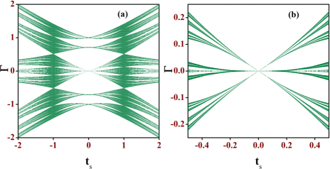
Figure 3: (Color online) (a) The self similar distribution of the inter-strand hopping against varying intra-strand hopping integral $t_{S}$ for a three strand ladder network and (b) magnified version of the original spectrum around the central zone. We have set $\epsilon_{i}=0$, $t_{L}=1$ and, $\chi_{L}=\chi_{S}=0$. Also, all the vertical couplings $\Gamma_{\alpha}$, $\Gamma_{\beta}$ and $\Gamma_{\gamma}$ are set equal to $\Gamma$ for numerical calculation.

reveals that, we now have three independent Fibonacci chains with effective on site potentials [ $(\epsilon_{\alpha}\pm\sqrt{2}\Gamma_{\alpha})$, $(\epsilon_{\beta}\pm\sqrt{2}\Gamma_{\beta})$, $(\epsilon_{\gamma}\pm\sqrt{2}\Gamma_{\gamma})$ ], and [$\epsilon_{\alpha},\epsilon_{\beta},\epsilon_{\gamma}$]. Corresponding effective hopping integrals are $t_{L}\pm\sqrt{2}\chi_{L}$, $t_{S}\pm\sqrt{2}\chi_{S}$, and $t_{L}$ and $t_{S}$. Needless to say that, when considered individually, each set gives rise to the usual fragmented, Cantor set energy spectrum, typical of a one dimensional Fibonacci chain. The actual spectrum of the three strand ladder is then obtained by convolving the individual spectra.

Before we end this section we draw the attention of the reader to one pertinent issue regarding the nature of the eigenstates of the full Fibonacci mesh that one can guess from the decoupled equations. We should note that, as the wave functions $\phi_{i}$’s in the new basis are each a linear combination of the earlier amplitudes $\psi_{i}$, localized character of any of the $\phi_{i}$’s will prevail only when every individual $\psi_{i}$ contributing to that particular $\phi_{i}$ will be localized. On the other hand, if, by certain correlation, one can make at least one of the $\psi_{i}$’s extended in character, it will render the entire linear combination, $\phi_{i}=\sum_{j}\psi_{j}$ extended. that is, at least one of the independent ‘channels’ will contribute totally transparent states.

III Density of states using the RSRG method

For an arbitrary $N$-strand Fibonacci strip we use the standard RSRG decimation using the potential matrices $\tilde{\epsilon_{i}}$ and the hopping matrices $\tilde{t_{ij}}$. The decimation is implemented by ‘folding’ the multi-strand strip using the growth rule in the reverse direction, viz., $LS\rightarrow L^{\prime}$ and $L\rightarrow S^{\prime}$. The RSRG recursion relations are easily obtained as,

$$\tilde{\epsilon}_{\alpha,n+1} = \tilde{\epsilon}_{\gamma,n}+\tilde{t}_{S,n}^{T}(E.I-\tilde{\epsilon}_{\beta,n})^{-1}\tilde{t}_{S,n}+\tilde{t}_{L,n}(E.I-\tilde{\epsilon}_{\beta,n})^{-1}\tilde{t}_{L,n}^{T}$$

$$\tilde{\epsilon}_{\beta,n+1} = \tilde{\epsilon}_{\gamma,n}+\tilde{t}_{S,n}^{T}(E.I-\tilde{\epsilon}_{\beta,n})^{-1}\tilde{t}_{S,n}$$

$$\tilde{\epsilon}_{\gamma,n+1} = \tilde{\epsilon}_{\alpha,n}+\tilde{t}_{L,n}(E.I-\tilde{\epsilon}_{\beta,n})^{-1}\tilde{t}_{L,n}^{T}$$

$$\tilde{t}_{L,n+1} = \tilde{t}_{L,n}(E.I-\tilde{\epsilon}_{\beta,n})^{-1}\tilde{t}_{S,n}$$

$$\tilde{t}_{S,n+1} = \tilde{t}_{L,n}$$ (11)

With a small imaginary part added to the energy $E$, the matrix elements of the hopping matrix $\tilde{t_{L}}$ and $\tilde{t_{S}}$ flow to zero after a finite number of iterations. The Green’s function matrix $\tilde{G}(E)$ is then obtained from the equation $\tilde{G}(E+i\eta)=[(E+i\eta).I-\epsilon_{i}^{*}]^{-1}$, where the subscript $i=\alpha$, $\beta$ or $\gamma$, and the ‘asterix’ denotes the fixed point value of the corresponding on-site potential. The diagonal elements of the Green’s function matrix provide the density of states at the vertices on an $\alpha$, $\beta$ or a $\gamma$ strand.

III.0.1 The role of interstrand coupling

We make an interesting observation to begin with. We fix $t_{L}=1$, and look for the nature of distribution of the mutual values of the intra-strand hopping $t_{S}$ and the inter-strand one, that is $\Gamma_{i}$, with $\chi_{L}=\chi_{S}=0$ for the time being. For simplicity we set $\Gamma_{\alpha}=\Gamma_{\beta}=\Gamma_{\gamma}=\Gamma$, and vary both $t_{S}$ and $\Gamma_{i}$ within $[-2,2]$ in units of $t_{L}$. The changing values of $\Gamma$, in a naive way, correspond to the proximity of the strands of the ladder.

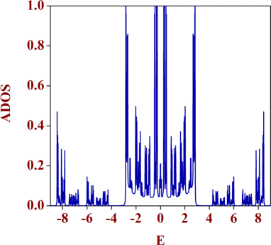
Figure 4: (Color online) Average density of states of a $3$-strand Fibonacci strip with correlated parameters. $\chi_{L}=1+1/\sqrt{2}$ and $\chi_{S}=1+\sqrt{2}$. We have chosen $\epsilon_{i}=0$ for $i=\alpha$, $\beta$, $\gamma$ and $\delta$, and $t_{L}=1$ and $t_{S}=2$. Energy is measured in units of $t_{L}$.

The plot in Fig. 3 depicts the $(\Gamma$, $t_{S})$ parameter subspace for which we get a non-zero density of states of the full three-strand Fibonacci ladder. The density of states has been obtained by using the recursion relations Eq. 11. It is interesting to observe that the distribution of the inter-strand tunnel hopping displays a three subband, self similar, fractal character. In Fig. 3(b) we have blown up an area around the origin to highlight the trifurcating character of the distribution.

III.0.2 Engineering absolutely continuous bands and extended wavefunctions

The strength of the decoupling scheme lies in its ability to engineer absolutely continuous energy bands even in such a system which doesn’t have any translational invariance. We justify the claim by pointing out to the fact that, for example, in Eq. (8), if one sets $\epsilon_{\alpha}-\sqrt{2}\Gamma_{\alpha}=\epsilon_{\beta}-\sqrt{2}\Gamma_{\beta}=\epsilon_{\gamma}-\sqrt{2}\Gamma_{\gamma}$, and $t_{L}-\sqrt{2}\chi_{L}=t_{S}-\sqrt{2}\chi_{S}$, then the set of Eq, (8) represents a perfectly ordered lattice. The energy eigenvalues of this effectively periodic chain form an absolutely continuous band with the pseudoparticle states extended, Bloch-like. The band is centered at $E=\epsilon_{\alpha}-\sqrt{2}\Gamma_{L}$, and extends from $E=\epsilon_{\alpha}-\sqrt{2}\Gamma_{L}-2(t_{L}-\sqrt{2}\chi_{L})$ to $E=\epsilon_{\alpha}-\sqrt{2}\Gamma_{L}+2(t_{L}-\sqrt{2}\chi_{L})$. It is to be noted that, such a correlation does not restrict the individual values of the potentials $\epsilon_{i}$, and the inter-strand hopping integrals $\Gamma_{i}$ from being chosen from any desired distribution. We are only demanding that the difference $\epsilon_{i}-\sqrt{2}\Gamma_{i}$ be kept constant. Similar is the case with the difference $t^{k}_{ij}-\sqrt{2}\chi^{k,k\pm 1}_{ij}$. Similar observation is made with respect to Eq. (10), where the correlations needed for the creation of an absolutely continuous band are, $\epsilon_{\alpha}+\sqrt{2}\Gamma_{\alpha}=\epsilon_{\beta}+\sqrt{2}\Gamma_{\beta}=$ $\epsilon_{\gamma}+\sqrt{2}\Gamma_{\gamma}$, and $t_{L}+\sqrt{2}\chi_{L}=t_{S}+\sqrt{2}\chi_{S}$.

In Fig. 4 we show the density of states of a three-strand Fibonacci strip with $\epsilon_{i}=0$, and with the above correlations respectively. We have taken, without any loss of generality, $\Gamma_{\alpha}=\Gamma_{\beta}=\Gamma_{\gamma}=0$, just to set the center of the spectrum at $E=0$, and the inter-strand coupling survives through the diagonal hopping integrals alone. It is easily understood that at a time only one of the two equations, viz., Eq. (8) or Eq. (10) can be made to contribute an absolutely continuous band populated by extended Bloch like states only. The remaining two equations will populate the spectrum with critical eigenstates, characteristic of a Fibonacci chain. However, if some of the critical states happen to be occupying part of the spectrum that falls within the band of extended wave functions, then they will lose their critical identity and become a part of the extended family.

Figure 5: (Color online) Average density of states of a $4$-strand Fibonacci strip with correlated parameters. $\chi_{L}=1+2/(\sqrt{5}+1)$ and $\chi_{S}=1+4/(\sqrt{5}+1)$. We have chosen $\epsilon_{i}=0$ for $i=\alpha$, $\beta$, $\gamma$ and $\delta$, and $t_{L}=1$ and $t_{S}=2$. Energy is measured in units of $t_{L}$.

This is precisely what happens in Fig. 4. We have set the correlation between the nearest and next nearest neighbor (along the diagonals) hopping integrals as, $t_{L}-\sqrt{2}\chi_{L}=t_{S}-\sqrt{2}\chi_{S}$. With $t_{L}=1$, $t_{S}=2$, $\chi_{L}=1+1/\sqrt{2}$ and $\chi_{S}=1+\sqrt{2}$, Eq. (8) represents a periodic chain of atomic sites with absolutely continuous band of extended states lying between $-2\sqrt{2}\leq E\leq 2\sqrt{2}$. Needless to say that, the two other equations, viz. Eq. (9) and Eq. (10) still represent two independent Fibonacci chains giving rise to ‘critical’ eigenstates. The full spectrum, as obtained from the RSRG recursion relations and the Green’s functions reproduce the absolute

Figure 6: (Color online) Density of states of a $5$-strand Fibonacci strip with an embedded periodic chain in the $3$rd strand. The values of the parameters are $\epsilon_{i}=0,i=\alpha$, $\beta$ and $\gamma$, $t_{L}=1$, $t_{S}=2$, $\chi_{L}=0=\chi_{S}$. The vertical couplings are (a) $\Gamma_{\alpha}=\Gamma_{\beta}=\Gamma_{\gamma}=0.2$, (b) $\Gamma_{\alpha}=\Gamma_{\beta}=\Gamma_{\gamma}=1$, (c) $\Gamma_{\alpha}=0.2$, $\Gamma_{\beta}=\Gamma_{\gamma}=0.5$ and (d) $\Gamma_{\alpha}=1$, $\Gamma_{\beta}=\Gamma_{\gamma}=0.5$. All the atomic sites of the extended defect chain have the same on-site potential $\epsilon=0$ and same hopping integral $t=1$.

continuum exactly over the energy regime, as extracted from the decoupled Eq. (8).

The ‘extendedness’ of the states has been verified by picking up arbitrary energy eigenvalues from inside the central portion ($-3<E<3$) in Fig. 4, and observing the flow of the hopping integrals under successive RSRG iteration steps, with the imaginary part of the energy set equal to zero. For all such energy eigenvalues the hopping integrals kept on oscillating without converging to zero for an arbitrary number of loops. This is an indication that the corresponding Wannier orbitals have finite overlap over arbitrarily large distances - a distinct signature of the extended character of the eigenfunction.

A similar test has been carried out to examine the nature of eigenstates populating the subbands at the flanks. We have encountered a whole bunch of eigenvalues for which the hopping integrals ultimately flow to zero, but only after a large number of RSRG iterations. This is suggestive of the fact that the corresponding eigenfunctions at least have very large localization lengths, if not ‘extended’ (if we consider a practical situation). It should be mentioned that, we have used the decoupled equations only to extract the region of the central (in this case) continuous subband. The density of states presented in every figure is obtained by using the RSRG method on the full multi-strand Fibonacci mesh.

Using the same set of values for the on-site potentials $\epsilon_{i}$ and the inter-strand vertical hopping $\Gamma_{i}$, $i=\alpha$, $\beta$, and $\gamma$, we present the DOS spectrum for the $4$-strand Fibonacci ladder in Fig. 5. Following the prescription laid out above, it is now straightforward to understand that the change of basis decouples this relatively complicated system into four independent linear chains, each representing the difference equation for the ‘mixed’ states, viz., $\phi_{i}=\sum_{N}\psi_{i,N}$. Each individual equation represents, as before, ‘pure’ Fibonacci quasiperiodic chains with both the effective on-site potentials and the hopping integrals arranged in Fibonacci sequence, and the spectrum offered by each one of them is a fragmented Cantor set, with the wave functions ‘critical’ in general, exhibiting a power-law localization and the usual multifractality. In Fig. 5 the spectrum is a mixed one, the central part being composed of an absolutely continuous band populated by extended eigenstates only. This continuum is a result of the correlation between $t_{L}$, $\chi_{L}$ and $t_{S}$, $\chi_{S}$ in a manner similar to the case of a three-strand ladder. The central part is flanked by fragmented subbands populated by localized eigenfunctions.

We have tested the extendedness of the wavefunctions in this case also in regions which appear to be continuous by observing the flow of the hopping integrals under the RSRG steps. The conclusions are the same as in the three-strand case discussed earlier.

IV The role of an ‘extended impurity’

We now examine the effect of an extended impurity segment, in the shape of an infinitely long periodically ordered chain embedded in the bulk of a multi-strand Fibonacci ladder. We refer to Fig. 2. No special correlations between the numerical values of the hopping integrals is introduced. This is an interesting situation when heterogeneity in the system is introduced at the minimal level. The influence of coupling transport channels which exhibit completely different localization properties has already provided exciting results  markus , and the present study draws inspiration out of this.

We present the results of the DOS for a five-strand ladder network where the central strand is an ordered chain, extending up to infinity along the $x$-direction. We have not gone for any special correlation between the hopping integrals as in the earlier situations. Yet, for weak (compared to $t_{S}$) tunnel hopping $\Gamma_{i}$, the panel (a) in Fig. 6 brings out the presence of a broad continua in segments in the DOS spectrum. Such zones turn out to be populated by extended eigenfunctions only, as we have tested by observing the flow of the hopping integrals under successive steps of renormalization. The flanks of the central continuum are populated by localized states, for which the hopping integrals, under RSRG iteration, flow to zero after a finite (in some cases a remarkably large number even) number of iterations. With increasing values of $\Gamma_{i}$ the feature still persists, unless, for a large enough value, the spectrum fragments into sharply localized subclusters with the hopping integrals flowing to zero after a nominal number of RSRG iteration. However, the typical trifurcating pattern observed in the DOS of a one dimensional Fibonacci chain (transfer model) is absent.

V Concluding remarks

We have studied the electronic properties of a quasi-one dimensional quasiperiodic lattice in the form of a multi-strand ladder network. We have specifically chosen a Fibonacci seqeunce to generate such a structure and have investigated the spectral characters by evaluating the densities of states using a real space renormalization group formalism. A commutation relation between the potential and the hopping matrices has been exploited to work out special correlations between the numerical values of various hopping integrals by virtue of which one can create absolutely continuous subbands of extended eigenstates only. This aspect provides a non-trivial variation over the canonical case of Anderson localization. Finally, the insertion of a line impurity is shown to lead to a gross change in the spectral character, leading to the generation of extended eigenfunctions as well.

- (1) P. W. Anderson, Phys. Rev. 109, 1492 (1958).
- (2) B. Kramer and A. MacKinnon, Rep. Prog. Phys. 56, 1469 (1993).
- (3) E. Abrahams, P. W. Anderson, D. C. Licciardello, and T. V. Ramakrishnan, Phys. Rev. Lett. 42, 673 (1979).
- (4) A. Christ, Y. Ekinci, H. H. Solak, N. A. Gippius, S. G. Tikhodeev, and O. J. F. Martin, Phys. Rev. B 76, 201405(R) (2007).
- (5) F. Rüting, Phys. Rev. B 83, 115447 (2011).
- (6) J. O. Vasseur, P. A. Deymier, G. Frantziskonis, G. Hong, B. Djafari-Rouhani, and L. Dobrzynski, J. Phys.: Condens. Matter 10, 6051 (1998).
- (7) I. O. Barinov, A. P. Alodzhants, and S. M. Arakelyan, Quantum Electron. 39, 685 (2009).
- (8) E. Yablonovitch, Phys. Rev. Lett. 58, 2059 (1987).
- (9) S. John, Phys. Rev. Lett. 58, 2486 (1987).
- (10) Y. Gilead, M. Verbin, and Y. Silberberg, Phys. Rev. Lett. 115, 133602 (2015).
- (11) J. Svozilík, J. Peřina, Jr., and J. P. Torres, Phys. Rev. A 89, 053808 (2014).
- (12) D. H. Dunlap, H-L. Wu, and P. W. Phillips, Phys. Rev. Lett. 65, 88 (1990).
- (13) W. Zhang and S. E. Ulloa, Phys. Rev. B 69, 153203 (2004).
- (14) S. Sil, S. K. Maiti, and A. Chakrabarti, Phys. Rev. B 78, 113103 (2008).
- (15) A. Rodriguez, A. Chakrabarti, and R. A. Römer, Phys. Rev. B 86, 085119 (2012).
- (16) B. Pal, S. K. Maiti, and A. Chakrabarti, Europhys. Lett. 102, 17004 (2013).
- (17) B. Pal and A. Chakrabarti, Eur. Phys. J. B 85, 307 (2012).
- (18) A. Chakrabarti, S. N. Karmakar, and R. K. Moitra, Phys. Rev. B 39, 9730 (1989).
- (19) M. Kohmoto, B. Sutherland, and C. Tang, Phys. Rev. B 35, 1020 (1987).
- (20) H. -Y. Xie, V. E. Kravtsov, and M. Müller, Phys. Rev. B 86, 014205 (2012).