On the Irregularity of Some Molecular Structures

Abstract

Measures of the irregularity of chemical graphs could be helpful for QSAR/QSPR studies and for the descriptive purposes of biological and chemical properties, such as melting and boiling points, toxicity and resistance. Here we consider the following four established irregularity measures: the irregularity index by Albertson, the total irregularity, the variance of vertex degrees and the Collatz-Sinogowitz index. Through the means of graph structural analysis and derivation, we study the above-mentioned irregularity measures of several chemical molecular graphs which frequently appear in chemical, medical and material engineering, as well as the nanotubes: $TUC_{4}C_{8}(S)$, $TUC_{4}C_{8}(R)$, Zig-Zag $TUHC_{6}$, $TUC_{4}$, Armchair $TUVC_{6}$, then dendrimers $T_{k,d}$ and the circumcoronene series of benzenoid $H_{k}$. In addition, the irregularities of Mycielski’s constructions of cycle and path graphs are analyzed.

Keywords: Irregularity indices, molecular structures, nanotube, dendrimer, circumcoronene of benzenoid

1 Introduction

Nowadays, due to the increasing need of engineering applications in the fields of transportation, aerospace, military and other various industrial fields, there has been an accelerating demand for high performance materials. The deterioration of the global environment makes the original virus mutate at a greater pace, causing new diseases to emerge, which increase mankind’s demand for new drugs. It is with the continuous improvements on chemical technology that the new materials and new drugs are discovered. Each year, these ever-increasing supply of new drugs and materials meets the human needs in the industrial and medical fields. However, with the new chemical substances there is a real necessity for a lot of chemical experiments to test their properties, which would require a lot of researchers, material and financial resources. On the other hand, in Southeast Asia, Latin America, Africa among other developing countries and regions, their governments cannot invest enough money to organize people, purchase equipment and reagents to detect the properties of these new compounds, which is one of the main reasons why these countries fall behind in the fundamental industrial and medical fields. Fortunately, early studies have shown that properties of the compound and its molecular structure are inextricably linked. By studying the corresponding molecular structure of the material and drug, we can understand the chemical and pharmacological properties of the compound. This discovery makes theoretical chemistry an important branch of chemistry that attracts more and more attention.

In standard theoretical chemistry, the chemical molecular structure is expressed as a graph: each vertex denotes an atom of a molecule and each edge between the corresponding vertices expresses covalent bounds between the atoms. This graph obtained from a chemical molecular structure is often called the molecular graph. A topological chemical index defined on molecular graph $G$ can be regarded as a real-valued function $f:G\to\mathbb{R}$ which assigns each molecular structure to a real number. In the past four decades, researchers in chemical and mathematical science have introduced several important indices, such as the Zagreb index, the PI index, the eccentric index, the atom-bond connectivity index, the forgotten index and the Wiener index e.g, to predict the characteristics of drugs, nanomaterials and other chemical compounds. There were several articles contributing to manifest these topological indices of special molecular structures in nanomaterials, chemical, biological and pharmaceutical engineering and in extremal molecular structures [3, 15, 16, 17, 18].

Let $G$ be a simple undirected graph with $|V(G)|=n$ vertices and $|E(G)|=m$ edges. The degree of a vertex $v$ in $G$ is the number of edges incident with $v$ and it is denoted by $d_{G}(v)$. A graph $G$ is regular if all its vertices have the same degree, otherwise it is irregular. In many applications and problems in chemistry and pharmacy, it is of great importance to know how irregular a given graph is.

There are many ways to define a regularity of a graph. Let ${{\rm imb}}(e)=\left|d_{G}(u)-d_{G}(v)\right|$ be the imbalance of an edge $e=uv\in E$. In [7], Albertson defined the irregularity of $G$ as

$${{\rm irr}}(G)=\sum_{e\in E(G)}{{\rm imb}}(e)=\sum_{uv\in E(G)}|d_{G}(u)-d_{G}(v)|.$$ (1)

It is shown in [7] that for a graph $G$, ${{\rm irr}}(G)<4n^{3}/27$ and that this bound can be approached arbitrarily close. This bound was slightly improved in [1]. Albertson also presented upper bounds on irregularity for bipartite graphs, triangle-free graphs and a sharp upper bound for trees. Some claims about bipartite graphs given in Albertson [7] have been formally proved in Henning and Rautenbach [22]. Related to Albertson’s work is the work of Hansen and Mélot [21], who characterized the graphs with $n$ vertices and $m$ edges with maximal irregularity.

In [2], a new measure of irregularity of a graph, so-called the total irregularity of a graph, was defined as

$${{\rm irr}_{t}}(G)=\frac{1}{2}\sum_{u,v\in V(G)}\left|d_{G}(u)-d_{G}(v)\right|.$$ (2)

Moreover, in [2] a sharp upper bound of the total irregularity ${{\rm irr}_{t}}$ was given and the graphs of small and maximal total irregularity were characterized. The comparison between the irregularity ${{\rm irr}}$ and the total irregularity ${{\rm irr}_{t}}$ of a graph was studied in [14].

Two other most frequently used graph topological indices that measure how irregular a graph is, are the variance of degrees and the Collatz-Sinogowitz index [12]. For graph $G$ let $\lambda_{1}$ be the largest eigenvalue of the adjacency matrix $A=(a_{ij})$ (with $a_{ij}=1$ if vertices $i$ and $j$ are joined by an edge and $0$ otherwise). A sequence of non-negative integers $d_{1},...,d_{n}$ is a graphic sequence, or a degree sequence, if there exists a graph $G$ with $V(G)=\{v_{1},...,v_{n}\}$ such that $d(v_{i})=d_{i}$. By $n_{i}$ we denote the number of vertices of degree $i$ for $i=1,2,\dots,n-1$ and by $d_{1},...,d_{n}$ the degree sequence of the graph $G$, where $n_{i}$ is the number of vertices of degree $i$ for $i=1,2,\cdots,n-1$. The variance ${\rm Var}({\it G})$ of the vertex degrees of the graph $G$ is

$${\rm Var}({\it G}) = \frac{1}{n}\sum^{n}_{i=1}d^{2}_{i}-\frac{1}{n^{2}}(\sum^{n}_{i=1}d_{i})^{2}=\frac{1}{n}\sum_{i=1}^{n-1}n_{i}\left(i-\frac{2m}{n}\right)^{2}.$$ (3)

The graph $G=(V,E)$ of order $n=|V(G)|$, size $m=|E(G)|$, maximum degree $\Delta$ and a real $(0,1)-$adjacency matrix $A(G)=(a_{ij})$, where $a_{ij}=1$ if the vertices $i$ and $j$ are adjacent otherwise $a_{ij}=0$. Since $A$ is symmetric, its eigenvalues $\lambda_{1},\cdots,\lambda_{n}$ are real and we assume that $\lambda_{1}\geq\lambda_{2}\geq\dots\ \geq\lambda_{n}$. Accordingly we write $\lambda_{i}(G)=\lambda_{i}(A)=\lambda_{i}$, $(i=1,\cdots,n)$. The eigenvalues $\lambda_{1},\cdots,\lambda_{n}$ refers to the spectrum of $G$. The largest eigenvalue $\lambda_{1}$ is called the spectral radius of $A$. For the connected graph $G$, the adjacency matrix $A$ is irreducible and so there exists a unique positive unit eigenvector corresponding to $\lambda_{1}$ (i.e., $\lambda_{1}$ has multiplicity $1$).

The Cartesian product $G\,\Box\,H$ of two simple undirected graphs $G$ and $H$ is the graph with the vertex set $V(G\,\Box\,H)=V(G)\times V(H)$ and the edge set $E(G\,\Box\,H)=\{(u_{i},v_{k})(u_{j},v_{l}):[(u_{i}u_{j}\in E(G))\wedge$ $(v_{k}=v_{l})]\vee[(v_{k}v_{l}\in E(H))\wedge(u_{i}=u_{j})]\}$.

Collatz and Sinogowitz  [12] introduced an irregularity index ${\rm CS}(G)$ and defined it as

$${\rm CS}(\it{G}) = \lambda_{1}(G)-\overline{d}(G)=\lambda_{1}(G)-\frac{2m}{n},$$ (4)

where $\overline{d}(G)=\sum^{n}_{i=1}d_{i}/n=2m/n$ denotes the average degree of the graph $G$. Results of comparing ${{\rm irr}}$, ${\rm CS}$ and ${\rm Var}$ are presented in [8, 13, 19].

Mukwembi [24, 25] introduced an irregularity index ${\rm t}(\it{G})$ of the graph $G$, as the number of distinctive terms in the degree sequence of $G$. Clearly, for any connected graph $G$ with maximum degree $\Delta$, the irregularity index ${\rm t}((\it{G})$ satisfies ${\rm t}(\it{G})\leq\Delta(\it{G})$. Other attempts to determine how irregular graph are [4, 5, 6, 9, 10, 11, 20, 23].

Although there have been several contributions on degree-based and distance-based indices chemical molecular graphs, the studies on irregularity related indices for certain special chemical structures are still largely limited. In [26] the irregularity of chemical trees with respect to the variance of vertex degrees and the Collatz-Sinogowitz index was investigated. The aim of the research presented in this paper is to extend that work by computing and comparing the irregularities of some relevant chemical graphs by the four, above metionied, irregularity measures. Specifically, the contribution of our paper is three-fold. First, we present the irregularities of five kinds of nanostructure: $TUC_{4}C_{8}(S)$, $TUC_{4}C_{8}(R)$, Zig-Zag $TUHC6$, $TUC_{4}$, Armchair $TUVC6$ nanotubes. Then, the irregularities of dendrimer $T_{k,d}$ and circumcoronene series of benzenoid $H_{k}$ are deduced. At last, we anylize the irregularities of Mycielski’s constructors $M(C_{n})$ and $M(P_{n})$.

2 Irregularities of some chemical graphs

2.1 $TUC_{4}C_{8}(S)[p,q]$ and $TUC_{4}C_{8}(R)[p,q]$ nanotubes

A $TUC_{4}C_{8}(S)$ nanotube can be constructed by rolling a lattice of carbon atoms as it is depicted in Figure 1. The two-dimensional lattice (Figure 1(b)) is made by alternating squares $C_{4}$ and octagons $C_{8}$. We denote the number of squares in each row by $p$ and the number of rows by $q$.

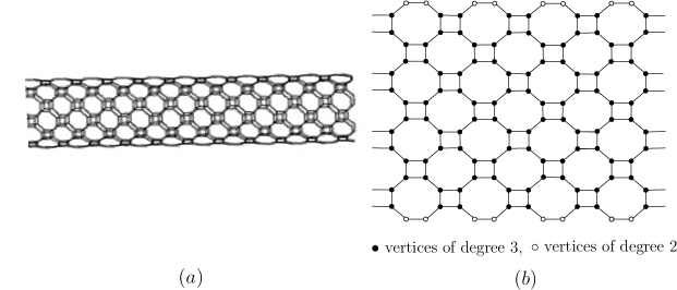
Figure 1: $(a)$ $3$D nanotube $TUC_{4}C_{8}(S)$, $(b)$ $2$D lattice of a $TUC_{4}C_{8}(S)[4,4]$.

Theorem 2.1.

Let $G=TUC_{4}C_{8}(S)[p,q]$ be a general $TUC_{4}C_{8}(S)$ nanotube. Then,

$${{\rm Var}}(G)=\frac{q-1}{q^{2}},\quad{{\rm CS}}(G)=\displaystyle{\lambda}_{1}(G)-3-\frac{1}{q},\quad{{\rm irr}}(G)=4p,\quad{{\rm irr}}_{t}(G)=8\,p^{2}(q-1).$$

Proof.

It holds that $|V(G)|=4pq$ and $|E(G)|=2p(3q-1)$. Let

$$V_{1}(G) = \{v\in V(G):d_{G}(v)=2\},$$

$$V_{2}(G) = \{u\in V(G):d_{G}(u)=3\},$$

$$E_{1}(G) = \{e=uv\in E(G):d_{G}(u)\neq d_{G}(v)\},$$

$$E_{2}(G) = \{e=uv\in E(G):d_{G}(u)=d_{G}(v)=2\},$$

$$E_{3}(G) = \{e=uv\in E(G):d_{G}(u)=d_{G}(v)=3\}.$$

Then,

$$|V_{1}(G)|=4p,$$

$$|V_{2}(G)|=4p(q-1),$$

$$|E_{1}(G)|=4p\mbox{ with }{\rm imb}(e)=1,$$

$$|E_{2}(G)|=2p\mbox{ with }{\rm imb}(e)=0,$$

$$|E_{3}(G)|=2p(3q-4)\mbox{ with }{\rm imb}(e)=0.$$

Hence, the variance ${\rm Var}(G)$, the Collatz-Sinogowitz index ${\rm CS}(G)$, the irregularity ${\rm irr}(G)$, and the total irregularity ${\rm irr}_{t}(G)$ of the nanotubes $TUC_{4}C_{8}(S)[p,q]$ are

$${\rm Var}(G) = \,\frac{1}{n}\,\sum\limits_{v\in V(G)}d^{2}_{G}(v)-\,\frac{1}{n^{2}}\,(\sum\limits_{v\in V(G)}d_{G}(v))^{2}$$

$$= \frac{1}{n}(\sum\limits_{v\in V_{1}(G)}d^{2}_{G}(v)+\sum\limits_{v\in V_{2}(G)}d^{2}_{G}(v))-\frac{1}{n^{2}}(\,\sum\limits_{v\in V_{1}(G)}d_{G}(v)+\,\sum\limits_{v\in V_{2}(G)}d_{G}(v)\,)^{2}$$

$$= \frac{1}{4pq}(16p+36\,p(q-1)\,)-\frac{1}{16p^{2}q^{2}}(8p+12p\,(q-1)\,)^{2}=\frac{q-1}{q^{2}}.$$

$${\rm CS}(G) = \lambda_{1}(G)-\overline{d}(G)=\lambda_{1}(G)-\frac{2m}{n}=\lambda_{1}(G)-\frac{2(2p(3q-1))}{4pq}=\lambda_{1}(G)-3-\frac{1}{q},$$

$${\rm irr}(G) = \sum\limits_{uv\in E(G)}\left|d_{G}(u)-d_{G}(v)\right|=\left(\sum\limits_{uv\in E_{1}(G)}+\sum\limits_{uv\in E_{2}(G)}+\sum\limits_{uv\in E_{3}(G)}\right)\left|d_{G}(u)-d_{G}(v)\right|=4p,$$

$${\rm irr}_{t}(G) = \,\frac{1}{2}\,\sum\limits_{u,v\in V(G)}\left|d_{G}(u)-d_{G}(v)\right|=\,\frac{1}{2}\,4p\,(q-1)(4p)=8\,p^{2}(q-1).$$

∎

A $TUC_{4}C_{8}(R)$ nanotube is depicted in Figure 2 and its two-dimensional lattice is illustrated in Figure 2(b).

Figure 2: $(a)$ $3$D nanotube $TUC_{4}C_{8}(R)$, $(b)$ $2$D lattice of a $TUC_{4}C_{8}(R)[4,4]$.

Theorem 2.2.

Let $G=TUC_{4}C_{8}(R)[p,q]$ be a general $TUC_{4}C_{8}(R)$ nanotube. Then,

$${{\rm Var}}(G)=\frac{2q-1}{4q^{2}},\quad{{\rm CS}}(G)=\lambda_{1}(G)-3-\frac{1}{2q},\quad{\rm irr}(G)=4p,\quad{\rm irr}_{t}(G)=2\,p^{2}(2q-1).$$

Proof.

We have that that $|V(G)|=4pq$ and $|E(G)|=p(6q-1)$.For

$$V_{1}(G) = \{v\in V(G):d_{G}(v)=2\},$$

$$V_{2}(G) = \{u\in V(G):d_{G}(u)=3\},$$

$$E_{1}(G) = \{e=uv\in E(G):d_{G}(u)\neq d_{G}(v)\},$$

$$E_{2}(G) = \{e=uv\in E(G):d_{G}(u)=d_{G}(v)=3\},$$

we have that

$$|V_{1}(G)|=2p,$$

$$|V_{2}(G)|=2p(2q-1),$$

$$|E_{1}(G)|=4p\mbox{ with }{\rm imb}(e)=1,$$

$$|E_{2}(G)|=p(6q-5)\mbox{ with }{\rm imb}(e)=0.$$

The four considered irregularity measures of the nanotubes $TUC_{4}C_{8}(R)[p,q]$ are

$${\rm Var}(G) = \,\frac{1}{n}\,\sum\limits_{v\in V(G)}d^{2}_{G}(v)-\,\frac{1}{n^{2}}\,(\sum\limits_{v\in V(G)}d_{G}(v))^{2}$$

$$= \frac{1}{n}(\sum\limits_{v\in V_{1}(G)}d^{2}_{G}(v)+\sum\limits_{v\in V_{2}(G)}d^{2}_{G}(v))-\frac{1}{n^{2}}(\,\sum\limits_{v\in V_{1}(G)}d_{G}(v)+\,\sum\limits_{v\in V_{2}(G)}d_{G}(v)\,)^{2}$$

$$= \frac{1}{4pq}(2^{2}(2p)+3^{2}(2p(2q-1)))-\frac{1}{16p^{2}q^{2}}(4p+3(2p(2q-1)))^{2}=\frac{2q-1}{4q^{2}}.$$

$${\rm CS}(G) = \lambda_{1}(G)-\overline{d}(G)=\lambda_{1}(G)-\frac{2m}{n}=\lambda_{1}(G)-\frac{2(p(6q-1))}{4pq}=\lambda_{1}(G)-3-\frac{1}{2q},$$

$${\rm irr}(G) = \sum\limits_{uv\in E(G)}\left|d_{G}(u)-d_{G}(v)\right|=\left(\sum\limits_{uv\in E_{1}(G)}+\sum\limits_{uv\in E_{2}(G)}\right)\left|d_{G}(u)-d_{G}(v)\right|=4p,$$

$${\rm irr}_{t}(G) = \,\frac{1}{2}\,\sum\limits_{u,v\in V(G)}\left|d_{G}(u)-d_{G}(v)\right|=\,\frac{1}{2}\,2p\,(2q-1)(2p)=2\,p^{2}(2q-1).$$

∎

The computation of the adjacency matrices of $TUC_{4}C_{8}(S)$ and $TUC_{4}C_{8}(R)$ (and the rest of the molecular structures considered in this work) as well as the computation of their corresponding largest eigenvalues were done in Matlab. The source code for computing the adjacencies matrices is given in the appendix. A comparison between the variance and Collatz-Sinogowitz of $TUC_{4}C_{8}(S)$ and $TUC_{4}C_{8}(R)$ for different values of $q$ is given in Figure 3. The variance of the nanotube $TUC_{4}C_{8}$ depends only on the number of rows $q$ (as shown in Theorems 2.1 and 2.2). The computations show that the Collatz-Sinogowitz index of $TUC_{4}C_{8}$ depends only on the number of rows $q$, too. $\lambda_{1}(TUC_{4}C_{8})$.

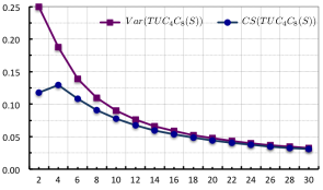
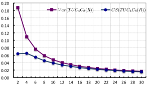
(a)	(b)

Figure 3: Comparison between ${\rm Var}$ and ${\rm CS}$ of $(a)$ $TUC_{4}C_{8}(S)$ and $(b)$ $TUC_{4}C_{8}(R)$.

2.2 $TUC_{4}(m,n)$ nanotube

$TUC_{4}(p,q)$ is a nanotube that can be obtained as Cartesian product of the $p-$path $P_{p}$ graph and the $q-$cycle graph $C_{q}$ (Figure 4). We denote the number of vertices in a row by $p$ and the number of vertices in a column by $q$.

Figure 4: $(a)$ Nanotubes $TUC_{4}[p,6]$, $(b)$ Nanotubes $TUC_{4}[8,4]$

Theorem 2.3.

Let $G=TUC_{4}(p,q)$. Then,

$${{\rm Var}}(G)=\frac{2(p-2)}{p^{2}},\quad{{\rm CS}}(G)=\lambda_{1}(G)-4+\frac{2}{p},\quad{\rm irr}(G)=2q,\quad{\rm irr}_{t}(G)=q^{2}(p-2).$$

Proof.

It holds that $|V(G)|=pq$ and $|E(G)|=q(2p-1)$. Let

$$V_{1}(G) = \{v\in V(G):d_{G}(v)=3\},$$

$$V_{2}(G) = \{u\in V(G):d_{G}(u)=4\},$$

$$E_{1}(G) = \{e=uv\in E(G):d_{G}(u)\neq d_{G}(v)\},$$

$$E_{2}(G) = \{e=uv\in E(G):d_{G}(u)=d_{G}(v)=3\},$$

$$E_{3}(G) = \{e=uv\in E(G):d_{G}(u)=d_{G}(v)=4\}.$$

Then,

$$|V_{1}(G)|=2q,$$

$$|V_{2}(G)|=(p-2)q,$$

$$|E_{1}(G)|=2q\mbox{ with }{\rm imb}(e)=1,$$

$$|E_{2}(G)|=2q\mbox{ with }{\rm imb}(e)=0,$$

$$|E_{3}(G)|=q(2p-5)\mbox{ with }{\rm imb}(e)=0.$$

Consequently, the four irregularity measures of the nanotubes $TUC_{4}(p,q)$ are

$${\rm Var}(G) = \,\frac{1}{n}\,\sum\limits_{v\in V(G)}d^{2}_{G}(v)-\,\frac{1}{n^{2}}\,(\sum\limits_{v\in V(G)}d_{G}(v))^{2}$$

$$= \frac{1}{n}(\sum\limits_{v\in V_{1}(G)}d^{2}_{G}(v)+\sum\limits_{v\in V_{2}(G)}d^{2}_{G}(v))-\frac{1}{n^{2}}(\,\sum\limits_{v\in V_{1}(G)}d_{G}(v)+\,\sum\limits_{v\in V_{2}(G)}d_{G}(v)\,)^{2}$$

$$= \frac{1}{pq}(3^{2}(2q)+4^{2}(p-2)q)-\frac{1}{p^{2}q^{2}}(3(2q)+4(p-2)q)^{2}=\frac{2(p-2)}{p^{2}}.$$

$${\rm CS}(G) = \lambda_{1}(G)-\overline{d}(G)=\lambda_{1}(G)-\frac{2m}{n}=\lambda_{1}(G)-\frac{2(q(2p-1))}{pq}=\lambda_{1}(G)-4+\frac{2}{p},$$

$${\rm irr}(G) = \sum\limits_{uv\in E(G)}\left|d_{G}(u)-d_{G}(v)\right|=\left(\sum\limits_{uv\in E_{1}(G)}+\sum\limits_{uv\in E_{2}(G)}+\sum\limits_{uv\in E_{3}(G)}\right)\left|d_{G}(u)-d_{G}(v)\right|=2q,$$

$${\rm irr}_{t}(G) = \,\frac{1}{2}\,\sum\limits_{u,v\in V(G)}\left|d_{G}(u)-d_{G}(v)\right|=\,\frac{1}{2}\,2q\,(p-2)q=q^{2}(p-2).$$

∎

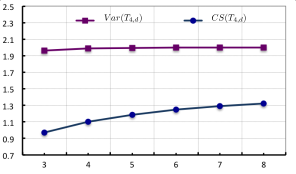
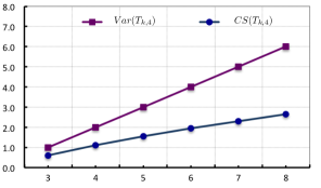
(a)	(b)
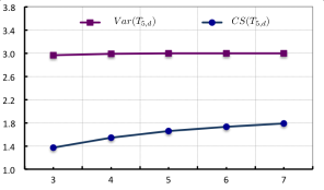
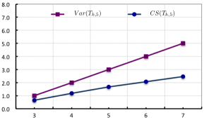
(c)	(d)

Figure 11: Comparison between ${\rm Var}$ and ${\rm CS}$ of $(a)$ $T_{4,d}$, $(b)$ $T_{k,4}$, $(c)$ $T_{5,d}$ and $(d)$ $T_{k,5}$.

A comparison between the variance and Collatz-Sinogowitz of $TUC_{4}$ for different values of $q$ is given in Figure 11. The variance of the nanotube $TUC_{4}$ depends only on the number of rows $p$ (as shown in Theorem 2.3).

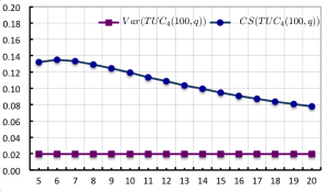
(a)	(b)

Figure 5: Comparison between ${\rm Var}$ and ${\rm CS}$ of $(a)$ $TUC_{4}(100,q)$ and $(b)$ $TUC_{4}(p,100)$.

Observe that ${\rm Var}(TUC_{4}(p,q))=2(p-2)/p^{2}$ and it is independent of $q$. Therefore, ${\rm Var}(TUC_{4}(100,q))$ has a constant value of $0.0196$. The calculations show that ${\rm CS}(TUC_{4}(p,100))$ is independent of $p$, respectively. However, the theoretical proof of this statement is missing.

2.3 Zig-Zag $TUHC_{6}$ nanotube

Let $G=TUHC_{6}[p,q]$ be a Zig-Zag polyhex nanotube, where $p$ is the number of hexagons in each row and $q$ is the number of Zig-Zag lines in the molecular graph of $G$, as it is depicted in Figure (6).

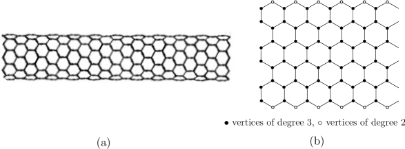
Figure 6: $(a)$ $3$D nanotube $TUHC6[p,q]$, $(b)$ $2$D lattice of a $TUHC6[6,6]$.

Theorem 2.4.

Let $G=TUHC_{6}[p,q]$ be a be a Zig-Zag polyhex nanotube. Then,

$${{\rm Var}}(G)=\frac{q-1}{q^{2}},\quad{{\rm CS}}(G)=\lambda_{1}(G)-3+\frac{1}{q},\quad{\rm irr}(G)=4p,\quad{\rm irr}_{t}(G)=4p^{2}(q-1).$$

Proof.

We have that $|V(G)|=2pq$ and $|E(G)|=p(3q-1)$. For

$$V_{1}(G) = \{v\in V(G):d_{G}(v)=2\},$$

$$V_{2}(G) = \{u\in V(G):d_{G}(u)=3\},$$

$$E_{1}(G) = \{e=uv\in E(G):d_{G}(u)\neq d_{G}(v)\},$$

$$E_{3}(G) = \{e=uv\in E(G):d_{G}(u)=d_{G}(v)=3\},$$

it follows that

$$|V_{1}(G)|=2p,$$

$$|V_{2}(G)|=2p(q-1),$$

$$|E_{1}(G)|=4p\mbox{ with }{\rm imb}(e)=1,$$

$$|E_{3}(G)|=p(3q-5)\mbox{ with }{\rm imb}(e)=0.$$

Thus, the variance ${\rm Var}(G)$, the Collatz-Sinogowitz index, the irregularity, and the total irregularity of the nanotubes $TUHC_{6}[p,q]$ are

$${\rm Var}(G) = \frac{1}{n}\,\sum\limits_{v\in V(G)}d^{2}_{G}(v)-\,\frac{1}{n^{2}}\,(\sum\limits_{v\in V(G)}d_{G}(v))^{2}$$

$$= \frac{1}{n}(\sum\limits_{v\in V_{1}(G)}d^{2}_{G}(v)+\sum\limits_{u\in V_{2}(G)}d^{2}_{G}(u))-\frac{1}{n^{2}}(\sum\limits_{v\in V_{1}(G)}d_{G}(v)+\sum\limits_{v\in V_{2}(G)}d_{G}(v)\,)^{2}$$

$$= \frac{1}{2pq}\,(2^{2}.2p+3^{2}.2p\,(q-1))-\frac{1}{4p^{2}\,q^{2}}\,(2.2p+3.2p(q-1))^{2}=\frac{q-1}{q^{2}}.$$

$${\rm CS}(G) = \lambda_{1}(G)-\overline{d}(G)=\lambda_{1}(G)-\frac{2m}{n}=\lambda_{1}(G)-\frac{2(p(3q-1))}{2pq}=\lambda_{1}(G)-3+\frac{1}{q},$$ (5)

$${\rm irr}(G) = \sum\limits_{e\in E(G)}\left|d_{G}(u)-d_{G}(v)\right|=\sum\limits_{e\in E^{\prime}(G)}\left|d_{G}(u)-d_{G}(v)\right|=4p.$$

$${\rm irr}_{t}(G) = \,\frac{1}{2}\,\sum\limits_{u\in V(G)}\sum\limits_{v\in V(G)}\left|d_{G}(u)-d_{G}(v)\right|=2p(2p(q-1))=4p^{2}(q-1).$$

∎

A comparison between the variance and Collatz-Sinogowitz of $TUHC_{6}[p,q]$ for different values of $q$ is given in Figure 7. The variance of the nanotube $TUHC_{6}$ depends only on the parameter $q$ (as shown in Theorem 2.4).

Figure 7: Comparison between ${\rm Var}$ and ${\rm CS}$ of $TUHC_{6}(100,q)$ .

2.4 $TUVC_{6}$ nanotube

Armchair $TUVC_{6}[p,q]$ nanotube can be constructed by rolling a lattice of carbon atoms comprised of $q$ columns and $p$ hexagons in each row (Figure 8).

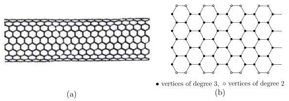
Figure 8: $(a)$ Armchair $3$D nanotube $TUVC6[p,q]$, $(b)$ $2$D lattice of a $TUVC6[4,9]$.

Theorem 2.5.

Let $G=TUVC_{6}[p,q]$ be an arbitrary armchair polyhex nanotube. Then,

$${{\rm Var}}(G)=\frac{2(q-2)}{q^{2}},\quad{{\rm CS}}(G)=\lambda_{1}(G)-3+\frac{2}{q},\quad{\rm irr}(G)=4p,\quad{\rm irr}_{t}(G)=4\,p^{2}(q-2).$$

Proof.

It holds that $|V(G)|=2pq$ and $|E(G)|=p(3q-2)$. Let,

$$V_{1}(G) = \{v\in V(G):d_{G}(v)=2\},$$

$$V_{2}(G) = \{u\in V(G):d_{G}(u)=3\},$$

$$E_{1}(G) = \{e=uv\in E(G):d_{G}(u)\neq d_{G}(v)\},$$

$$E_{2}(G) = \{e=uv\in E(G):d_{G}(u)=d_{G}(v)=2\},$$

$$E_{3}(G) = \{e=uv\in E(G):d_{G}(u)=d_{G}(v)=3\}.$$

Then,

$$|V_{1}(G)|=4p,$$

$$|V_{2}(G)|=2p(q-2),$$

$$|E_{1}(G)|=4p\mbox{ with }{\rm imb}(e)=1,$$

$$|E_{2}(G)|=2p\mbox{ with }{\rm imb}(e)=0,$$

$$|E_{3}(G)|=p(3q-8)\mbox{ with }{\rm imb}(e)=0.$$

Consequently, the all four irregularity measures: variance ${\rm Var}(G)$, Collatz-Sinogowitz index ${\rm CS}(G)$, irregularity ${\rm irr}(G)$, and the total irregularity ${\rm irr}_{t}(G)$ of the nanotubes $TUVC_{6}[p,q]$ are

$${\rm Var}(G) = \,\frac{1}{n}\,\sum\limits_{v\in V(G)}d^{2}_{G}(v)-\,\frac{1}{n^{2}}\,(\sum\limits_{v\in V(G)}d_{G}(v))^{2}$$

$$= \frac{1}{n}(\sum\limits_{v\in V_{1}(G)}d^{2}_{G}(v)+\sum\limits_{v\in V_{2}(G)}d^{2}_{G}(v))-\frac{1}{n^{2}}(\,\sum\limits_{v\in V_{1}(G)}d_{G}(v)+\,\sum\limits_{v\in V_{2}(G)}d_{G}(v)\,)^{2}$$

$$= \frac{1}{2pq}(16p+18\,p(q-2)\,)-\frac{1}{4p^{2}q^{2}}(8p+6p\,(q-2)\,)^{2}=\frac{2(q-2)}{q^{2}}.$$

$${\rm CS}(G) = \lambda_{1}(G)-\overline{d}(G)=\lambda_{1}(G)-\frac{2m}{n}=\lambda_{1}(G)-\frac{2(2p(3q-1))}{4pq}=\lambda_{1}(G)-3+\frac{2}{q},$$

$${\rm irr}(G) = \sum\limits_{uv\in E(G)}\left|d_{G}(u)-d_{G}(v)\right|=\left(\sum\limits_{uv\in E_{1}(G)}+\sum\limits_{uv\in E_{2}(G)}+\sum\limits_{uv\in E_{3}(G)}\right)\left|d_{G}(u)-d_{G}(v)\right|=4p,$$

$${\rm irr}_{t}(G) = \,\frac{1}{2}\,\sum\limits_{u,v\in V(G)}\left|d_{G}(u)-d_{G}(v)\right|=\,\frac{1}{2}\,4p\,(q-2)(2p)=4\,p^{2}(q-2).$$

∎

A comparison between the variance and Collatz-Sinogowitz of $TUVC_{6}[p,q]$ for different values of $q$ is given in Figure 9. The variance of the nanotube $TUVC_{4}$ depends only on the parameter $q$ (as shown in Theorem 2.5).

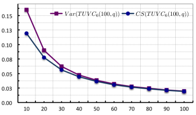
Figure 9: Comparison between ${\rm Var}$ and ${\rm CS}$ of $TUVC_{6}(100,q)$ .

2.5 $T_{k,d}$ dendrimer

A tree $T$ is a complete $k$-regular if every vertex has degree $1$ or $k$. A tree where all leaves are on the same distance to the root is called a balanced tree. By $T_{k,d}$, we denote a balanced $k$-regular tree whose leaves are at distance $d$ to the root of the tree. In chemical graph theory $T_{k,d}$ trees are also known as $T_{k,d}$ dendrimers. The $T_{k,d}$ dendrimers, for several different parameters of $k$ and $d$, are illustrated in Figure 10.

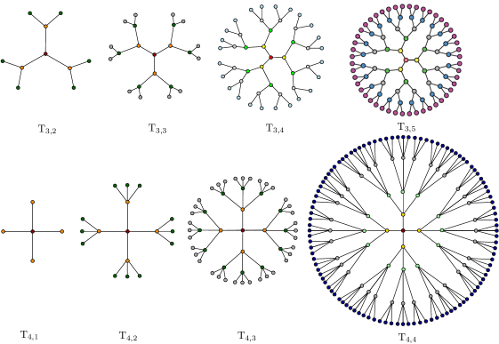
Figure 10: Molecular graphs of dendrimers $T_{3,0},\cdots,T_{3,3}$ and $T_{4,0},\cdots,T_{4,3}$.

Theorem 2.6.

Let $T_{k,d}$ be an a dendrimer. Then,

$$\begin{aligned} &{{\rm Var}}(T_{k,d})=\frac{k\,(k-2)\,(k-1)^{d}\,(k\,((k-1)^{d}-2)+2)}{(k(k-1)^{d}-2)^{2}},&&\quad{{\rm CS}}(T_{k,d})=\lambda_{1}(T_{k,d})-\frac{2k((k-1)^{d}-1)}{k(k-1)^{d}-2},\\ &{\rm irr}(T_{k,d})=k(k-1)^{d},&&\quad{\rm irr}_{t}(T_{k,d})=\frac{\,k^{2}\,(k-1)^{d}\,(\,(k-1)^{d-1}-2)}{2(k-2)}.\end{aligned}$$

Proof.

It can be easily computed that $|V(T_{k,d})|=(k(k-1)^{d}-2)/(k-2)$ and $|E(T_{k,d})|=k((k-1)^{d}-1)/(k-2)$. Let $V_{1}(T_{k,d})=$$\{v\in V(T_{k,d}):\;$$d_{T_{k,d}}(v)=1\}$, and $V_{2}(T_{k,d})=$$\{u\in V(T_{k,d}):\;$$d_{T_{k,d}}(u)=k\}$. Then $|V_{1}(T_{k,d})|=k(k-1)^{d-1}$ and $|V_{2}(T_{k,d})|=(k(k-1)^{d-1}-2)/(k-2)$. Let $E_{1}(T_{k,d})=$$\{uv\in E(T_{k,d}):\;$$d_{T_{k,d}}(u)\neq d_{T_{k,d}}(v)\}$. $|E_{1}({T_{k,d}})|=k(k-1)^{d-1}$, which is the number of leaves of $T_{k,d}$ with ${{\rm imb}(uv)}=k-1$ for all $uv\in E_{1}(G)$.

Thus, the variance, the Collatz-Sinogowitz index, the irregularity and total irregularity of $T_{k,d}$ are

$${\rm Var}(T_{k,d}) = \frac{1}{n}\,\sum\limits_{v\in V(T_{k,d})}d^{2}_{T_{k,d}}(v)-\,\frac{1}{n^{2}}\,(\sum\limits_{v\in V(T_{k,d})}d_{T_{k,d}}(v))^{2}$$

$$= \frac{1}{n}(\sum\limits_{v\in V_{1}(T_{k,d})}d^{2}_{T_{k,d}}(v)+\sum\limits_{u\in V_{2}(T_{k,d})}d^{2}_{T_{k,d}}(u))$$

$$-\frac{1}{n^{2}}(\sum\limits_{v\in V_{1}(T_{k,d})}d_{T_{k,d}}(v)+\sum\limits_{v\in V_{2}(T_{k,d})}d_{T_{k,d}}(v))^{2}$$

$$= \,\frac{k-2}{k(k-1)^{d}-2}\,\left(k\,(k-1)^{d-1}\,+\,k^{2}\,\frac{k\,(k-1)^{d-1}-2}{k-2}\right)$$

$$-\,\left(\,\frac{k-2}{k\,(k-1)^{d}-2}\right)^{2}\,\left(k\,(\,k-1)^{d-1}\,+\,k\,\frac{\,k\,(k-1)^{d-1}-2}{k-2}\,\right)^{2}$$

$$= \frac{k\,(k-2)\,(k-1)^{d}\,(k\,((k-1)^{d}-2)+2)}{(k(k-1)^{d}-2)^{2}}.$$

$${\rm CS}(T_{k,d}) = \lambda_{1}(T_{k,d})-\frac{2k((k-1)^{d}-1)}{k(k-1)^{d}-2}$$

$${\rm irr}(T_{k,d}) = \sum\limits_{e\in E(T_{k,d})}\left|d_{T_{k,d}}(u)-d_{T_{k,d}}(v)\right|=\sum\limits_{e\in E^{\prime}(T_{k,d})}\left|d_{T_{k,d}}(u)-d_{T_{k,d}}(v)\right|=k(k-1)^{d}.$$

$${\rm irr}_{t}(T_{k,d}) = \frac{1}{2}\,\sum\limits_{u,v\in V(T_{k,d})}\left|d_{T_{k,d}}(u)-d_{T_{k,d}}(v)\right|=\frac{\,k^{2}\,(k-1)^{d}\,(\,(k-1)^{d-1}-2)}{2(k-2)}.$$

∎

2.6 Circumcoronene series of benzenoid $H_{k}$

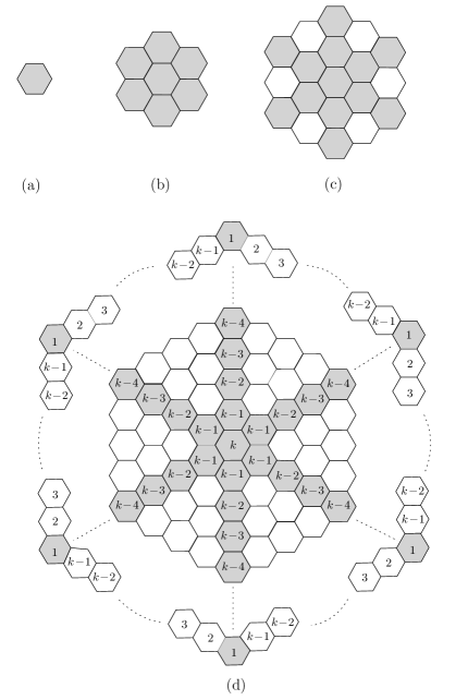
Figure 12: Circumcoronene series of benzenoid $H_{k}$. In $(a)$ Benzene $H_{1}=C_{6}$, $(B)$ Coronene $H_{2}=C_{6}(C_{6})$, $(c)$ Circumcoronene $H_{3}$ and (d) The circumcoronene series of benzenoid $H_{k}$.

In Figure (12) the circumcoronene series of benzenoid $H_{k}$, for $k=1,2,3$ and the circumcoronene series in the general case are depicted. The structures of this family of circumcoronene are presented as homologous series of benzenoid consisted several copy of benzene $C_{6}$ on circumference. Consider circumcoronene series of benzenoid $H_{k}$ for $k\geq 1$. It holds that $|V(H_{k})|=6k^{2}$ and $|E(H_{k})|=3k(3k-1)$.

Theorem 2.7.

Let $H_{k}$ be an a Circumcoronene. Then,

$${{\rm Var}}(H_{k})=\frac{k-1}{k^{2}},\quad{{\rm CS}}(H_{k},)=\lambda_{1}(T_{k,d})-\frac{3k-1}{k},\quad{\rm irr}(H_{k})=12(k-1),\quad{\rm irr}_{t}(H_{k})=36\,k^{2}\,(k-1).$$

Proof.

A direct calculations gives that $|V(H_{k})|=6k^{2}$ and $|E(H_{k})|=3k(3k-1)$. Let $V_{1}(H_{k})$$=\{v\in V(H_{k}):\;$$d_{H_{k}}(v)=2\}$, and $V_{2}(H_{k})=$$\{u\in V(H_{k}):\;$$d_{H_{k}}(u)=3\}$. Then $|V_{1}(H_{k})|=6k$ and $|V_{2}(H_{k})|=6k(k-1)$. Let $E_{1}(H_{k})=$$\{uv\in E(H_{k}):\;$$d_{H_{k}}(u)\neq d_{H_{k}}(v)\}$ with ${{\rm imb}(uv)}=1$ for all $uv\in E_{1}(H_{k})$, $E_{2}(H_{k})=$$\{uv\in E(H_{k}):\;$$d_{H_{k}}(u)=d_{H_{k}}(v)=2\}$ with ${{\rm imb}(uv)}=0$ for all $uv\in E_{2}(H_{k})$ and $E_{3}(H_{k})=$$\{uv\in E(H_{k}):\;$$d_{H_{k}}(u)=d_{H_{k}}(v)=3\}$ with ${{\rm imb}(uv)}=0$ for all $uv\in E_{3}(H_{k})$. Then $|E_{1}({H_{k}})|=12(k-1)$, $|E_{2}({H_{k}})|=6$ and $|E_{3}({H_{k}})|=3(3k-2)(k-1)$.

Thus, the variance, the Collatz-Sinogowitz index, the irregularity and total irregularity of $H_{k}$ are

$${\rm Var}(H_{k}) = \frac{1}{n}\,\sum\limits_{v\in V(H_{k})}d^{2}_{H_{k}}(v)-\,\frac{1}{n^{2}}\,(\sum\limits_{v\in V(H_{k})}d_{H_{k}}(v))^{2}$$

$$= \frac{1}{n}(\sum\limits_{v\in V_{1}(H_{k})}d^{2}_{H_{k}}(v)+\sum\limits_{u\in V_{2}(H_{k})}d^{2}_{H_{k}}(u))-\frac{1}{n^{2}}(\sum\limits_{v\in V_{1}(H_{k})}d_{H_{k}}(v)+\sum\limits_{v\in V_{2}(H_{k})}d_{H_{k}}(v))^{2}$$

$$= \,\frac{2^{2}(6k)+3^{2}(6k(k-1))}{6k^{2}}\,-\,\frac{(2(6k)+3(6k(k-1)))^{2}}{36k^{4}}$$

$$= \frac{9k-5}{k}-\frac{9k^{2}-6k+1}{k^{2}}$$

$$= \frac{k-1}{k^{2}}.$$

$${\rm CS}(H_{k}) = \lambda_{1}(H_{k})-\frac{2(3k(3k-1))}{6k^{2}}=\lambda_{1}(H_{k})-\frac{3k-1}{k}$$

$${\rm irr}(H_{k}) = \sum\limits_{e\in E(H_{k})}\left|d_{H_{k}}(u)-d_{H_{k}}(v)\right|=\sum\limits_{e\in E_{1}(H_{k})}\left|d_{H_{k}}(u)-d_{H_{k}}(v)\right|=12(k-1).$$

$${\rm irr}_{t}(H_{k}) = \frac{1}{2}\,\sum\limits_{u,v\in V(H_{k})}\left|d_{H_{k}}(u)-d_{H_{k}}(v)\right|=\frac{1}{2}\,\sum\limits_{u\in V_{1}(H_{k}),v\in V_{2}(H_{k})}\left|d_{H_{k}}(u)-d_{H_{k}}(v)\right|$$

$$= 36\,k^{2}\,(k-1).$$

∎

A comparison between the variance and Collatz-Sinogowitz of Circumcoronene series of benzenoid $H_{k}$ for different values of $k$ is given in Table 13.

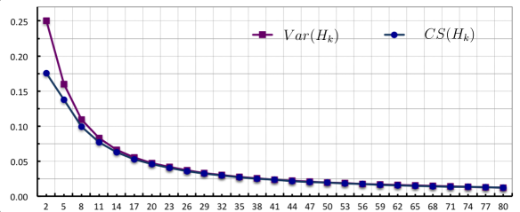
Figure 13: Comparison between ${\rm Var}$ and ${\rm CS}$ of Circumcoronene series of benzenoid $H_{k}$ for $k=2,5,\cdots,80$.

2.7 Mycielski’s construction $M(C_{n})$ and $M(P_{n})$

The Mycielski’s construction of a simple graph $G$ [27] produces a simple graph $M(G)$ containing $G$. Start with $G$ having vertex set $\{v_{1},v_{2},\cdots,v_{n}\}$, add vertices $U=\{u_{1},u_{2},\cdots,u_{n}\}$ and one more vertex $w$. Add edges to make $u_{i}$ adjacent to all $N_{G}(v_{i})$ and finally let $N(w)=U$. One iteration of Mycielski’s construction from the graph $C_{8}$ and $P_{8}$, where $C_{n}$, and $P_{n}$ are cycle and path of length $n$ respectively, yields the graph shown in Figure 14.

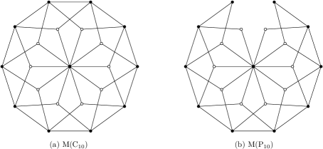
Figure 14: $(a)$ Mycielski’s graph $M(C_{8})$, $(b)$ Mycielski’s graph $M(P_{8})$.

Theorem 2.8.

Let $M(C_{n})$ and $M(P_{n})$ be Mycielski’s graph of cycle and path graphs with $n$ vertices. Then,

$$\begin{aligned} &{{\rm Var}}(M(C_{n}))=\frac{n(2\,n^{2}\,-13n+25)}{(2n+1)^{2}},&&\qquad{{\rm CS}}(M(C_{n}))=\lambda_{1}(M(C_{n}))-\frac{8n}{2n+1},\\ &{\rm irr}(M(C_{n}))=n(n-1),&&\qquad{\rm irr}_{t}(M(C_{n}))=n(3n-7),\\ &{{\rm Var}}(M(P_{n}))=\frac{(n-2)(2n^{2}-9n+35)}{(1+2n)^{2}},&&\qquad{{\rm CS}}(M(P_{n}))=\lambda_{1}(M(P_{n}))-\frac{2(4n-3)}{2n+1},\\ &{\rm irr}(M(P_{n}))=n^{2}-n+6,&&\qquad{\rm irr}_{t}(M(P_{n}))=(n-2)(3n+7).\end{aligned}$$

Straightforward calculations gives that $|V(M(C_{n}))|=2n+1$, $|E(M(C_{n}))|=4n$. Hence,

$${\rm Var}(M(C_{n})) = \frac{1}{2n+1}\sum\limits_{v\in V(M(C_{n}))}d^{2}_{M(C_{n})}(v)-\frac{1}{(2n+1)^{2}}\left(\sum\limits_{v\in V(M(C_{n}))}d_{M(C_{n})}(v)\right)^{2}$$

$$= \frac{1}{2n+1}\left(\sum\limits_{v\in V(M(C_{n}))}d^{2}_{M(C_{n})}(v)+\sum\limits_{u\in U}d^{2}_{M(C_{n})}(u)+n^{2}\right)$$

$$-\frac{1}{(2n+1)^{2}}\left(\sum\limits_{v\in V(M(C_{n}))}d_{M(C_{n})}(v)+\sum\limits_{u\in U}d_{M(C_{n})}(u)+n\right)^{2}$$

$$= \frac{4^{2}\,n+3^{2}\,n+n^{2}}{2n+1}-\left(\frac{4n+3n+n}{2n+1}\right)^{2}=\,\frac{n(2\,n^{2}\,-13n+25)}{(2n+1)^{2}}.$$

$${\rm CS}(M(C_{n})) = \lambda_{1}(M(C_{n}))-\frac{8n}{2n+1}$$

$${\rm irr}(M(C_{n})) = \sum\limits_{uv\in E(M(C_{n}))}\left|d_{M(C_{n})}(u)-d_{M(C_{n})}(v)\right|=n(n-3)+2n=n(n-1),$$

$${\rm irr}_{t}(M(C_{n})) = \,\frac{1}{2}\,\sum\limits_{u,\,v\in V(M(C_{n}))}\left|d_{M(C_{n})}(u)-d_{M(C_{n})}(v)\right|=n(n-4)+n(n-3)+n^{2}$$

$$= n(3n-7).$$

A direct calculations gives that $|V(M(P_{n}))|=2n+1$, $|E(M(P_{n}))|=4n-3$. The four considered irregularity measures have the following values:

$${\rm Var}(M(P_{n})) = \frac{1}{2n+1}\sum\limits_{v\in V(M(P_{n}))}d^{2}_{M(P_{n})}(v)-\frac{1}{(2n+1)^{2}}\left(\sum\limits_{v\in V(M(P_{n}))}d_{M(P_{n})}(v)\right)^{2}$$

$$= \frac{1}{2n+1}\left(\sum\limits_{v\in V(P_{n})}d^{2}_{M(P_{n})}(v)+\sum\limits_{u\in U}d^{2}_{M(P_{n})}(u)+n^{2}\right)$$

$$-\frac{1}{(2n+1)^{2}}\left(\sum\limits_{v\in V(P_{n})}d_{M(P_{n})}(v)+\sum\limits_{u\in U}d_{M(P_{n})}(u)+n\right)^{2}$$

$$= \frac{n^{2}+25n-34}{2n+1}-\left(\frac{8n-6}{2n+1}\right)^{2}=\frac{(n-2)(2n^{2}-9n+35)}{(2n+1)^{2}}.$$

$${\rm CS}(M(P_{n})) = \lambda_{1}(M(P_{n}))-\frac{2(4n-3)}{2n+1}$$

$${\rm irr}(M(P_{n})) = \sum\limits_{uv\in E(M(P_{n}))}\left|d_{M(P_{n})}(u)-d_{M(P_{n})}(v)\right|$$

$$= (n-2)(n-3)+2(n-2)+2(n-3)+8+2=n^{2}-n+6$$

$${\rm irr}_{t}(M(P_{n})) = \,\frac{1}{2}\,\sum\limits_{u\in V(M(P_{n}))}\sum\limits_{v\in V(M(P_{n}))}\left|d_{M(P_{n})}(u)-d_{M(P_{n})}(v)\right|$$

$$= (n-2)^{2}+(n-2)(n-3)+(n-2)(n-4)+(n-2)(4+4+4+2+2)$$

$$= (n-2)(3n+7).$$

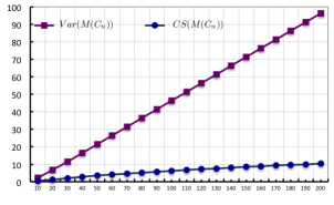
(a)	(b)

Figure 15: Comparison between ${\rm Var}$ and ${\rm CS}$ of Mycielski’s construction $(a)$ $M(C_{n})$ and $(b)$ $M(P_{n})$ for $n=10,20,\cdots,200$.

3 Concluding comments

With the rapid development of industry, including the medical field, a great deal of new chemical structures are being discovered and synthesized annually. This requires to spend more on detecting the characteristics of the many new drugs, materials and chemical compounds. Irregularity indices may help to measure the chemical, biological and nano properties which are widely popular in developing areas. In our article, in view of structure analysis and mathematical derivation, we report the irregularity related indices of certain molecular graphs which widely appear in nanoscience and drug structures.

To determine the CS index of the considered chemical structures, we have constructed the adjacency matrix of the underlying graph and then calculate its eigenvalues. Since the presented chemical compounds are very well structured, with repeating rules/patterns, we hope that it is possible to calculate the closed-form solutions of the CS index in those cases. This demanding task remains an open problem and could be considered for future work.

We conclude with the following conjecture that was deduced from the experimental part of this work.

Conjecture 3.1.

Let $G$ be a nanotube $TUC_{4}C_{8}(S)$, $TUC_{4}C_{8}(R)$, $TUHC_{6}$, $TUC_{4}$, $TUVC_{6}$ or circumcoronene series of benzenoid $H_{k}$, $k\geq 1$, and let $n$ be the order of $G$. Then,

$$\lim_{n\to\infty}({\rm Var}(G)-{\rm CS}(G))=0.$$

Appendix A Functions written in Matlab for computing the adjacency matrix of the considered molecular structures

A.1 A function for computing the adjacency matrix of $TUC_{4}C_{8}(S)[p,q]$ nanotube

• 01   function A = AdjMatrTUC4S4_S(p,q)
  02   n = 4*p*q;
  03   for i = 1 : n
  04       if rem(i , 4*p) == 0
  05           A(i , i - 4*p + 1) = 1;  A(i - 4*p + 1 , i) = 1;
  06       else
  07           A(i , i + 1) = 1;  A(i + 1 , i) = 1;
  08       end
  09       if (rem(i , 4) == 1 | rem(i , 4) == 2) && i < n - 4*p
  10           A(i , i + 4*p + 2) = 1;   A(i + 4*p + 2 , i) = 1;
  11       end
  12   end
  13   end
  

A.2 A function for computing the adjacency matrix of $TUC_{4}C_{8}(R)[p,q]$ nanotube

• 01   function A = AdjMatrTUC4S4_R(p,q)
  02   j = 3 ; k = 4; n = 4 * p * q;
  03   for i = 1 :  n
  04       if rem(i , 4) == 0
  05           A(i , i - 3) = 1; A(i - 3 , i) = 1;
  06           if i <= n - 4*p
  07               A(i , 4*p + i - 2) = 1;   A(4*p + i - 2 , i) = 1;
  08           end
  09       else
  10           A(i , i + 1) = 1;  A(i + 1 , i) = 1;
  11       end
  12       while j  <  n
  13           if j  ==  k*p  -  1
  14               A(j  ,  j - 4*p + 2) = 1;   A(j - 4*p + 2  ,  j) = 1;
  15               k = k + 4;
  16           else
  17               A(j  ,  j + 2)  =  1;   A(j + 2  ,  j)  =  1;
  18           end
  19           j = j + 4;
  20       end
  21   end
  

A.3 A function for computing the adjacency matrix of $TUC_{4}(m,n)$ nanotube

• 01   function A = AdjMatrTUC4(p,q)
  02   A  = [];
  03   for i = 1 :  p*(q - 1)
  04       A(i , i + p) = 1; A(i + p , i) = 1;
  05   end
  06   while i  <=  p*q  -  1
  07       for i = 1 :  p*q  - 1
  08           A(i , i + 1) = 1;  A(i + 1 , i) = 1;
  09           if rem(i,p) == 0
  10               A(i , i + 1) = 0;   A(i + 1 , i) = 0;
  11           end
  12       end
  13       i = i + 1;
  14   end
  15   for i = 1 : p : p*(q - 1) + 1
  16       A(i , i + p - 1) = 1;  A(i + p - 1 , i) = 1;
  17   end
  18   end
  

A.4 A function for computing the adjacency matrix of of Zig-Zag $TUHC_{6}$ nanotube

• 01   function A = AdjMatrTUHC(p,q)
  02   for j = 1 : 2*p*q
  03       if j == 2*p*q
  04           A(j , j - 1) = 1; A(j - 1 , j) = 1;
  05           A(j , j - 2*p + 1) = 1; A(j - 2*p + 1 , j) = 1;
  06       else
  07           A(j , j + 1) = 1;  A(j + 1 , j) = 1;
  08           if rem(j , 2*p) == 0
  09               A(j , j - 2*p + 1) = 1; A(j - 2*p + 1 , j) = 1;
  10               A(j , j + 1) = 0; A(j + 1 , j) = 0;
  11           end
  12       end
  13   end
  14   for j = 1 : q - 1
  15      if rem(j,2) ~= 0
  16          for i = 2*p*(j-1) + 1 :  2  :  2*p*j
  17               A(i , i + 2*p) = 1;  A(i + 2*p , i) = 1;
   18           end
  19       else
  20           for i = 2*p*(j-1) + 2  :  2  :  2*p*j
  21               A(i , i + 2*p) = 1;  A(i + 2*p , i) = 1;
  22           end
  23       end
  24   end
  25   end
  

A.5 A function for computing the adjacency matrix of Armchair $TUVC_{6}[p,q]$ nanotube

• 01   function A = AdjMatrTUVC(p,q)
  02   A = [ ];   j = 1;
  03   for i = 1 :  2*p*q - 2*p
  04       A(i , i+2*p) = 1;  A(i+2*p , i) = 1;
  05  end
  06   while j  <=  2*p*q - 1
  07       A(j , j+1) = 1;  A(j+1 , j) = 1;
  08       if rem(j+1 , 2*p) == 0 | rem(j+2 , 2*p) == 0
  09          if rem(j+2 , 4*p) == 0
  10              A(j+2 , j-2*p+3) = 1; A(j-2*p+3 , j+2) = 1;
  11           end
  12           j = j + 1;
  13       end
  14       j = j + 2;
  15    end
  16    end
  

A.6 A function for computing the adjacency matrix of dendrimers(k,d)

• 01   function A = AdjMatrDendrimers(k,d)
  02   Xsta = [];        Xend  = [];  A = [];
  03   Xsta(1) = 2;      Xend(1) = k+1;
  04   Xsta(2) = k + 2;  Xend(2) = k^2 + 1;
  05   A(1,2:k+1) = 1;    A(2:k+1,1) = 1;  %  -----   Distance = 1   -----
  06   t = 0;        %   -------------    Distance = 2    ----------------
  07   for i = 2 : k+1
  08       tt = k+2 + t*(k-1);
  09       A(i,tt:tt+(k-2)) = 1; A(tt:tt+(k-2),i) = 1;
  10       t = t +1;
  11   end
  12   for j = 3 : d   %   -------------  Distance >= 3    ---------------
  13       Xsta(j) = Xend(j-1) + 1;
  14       Xend(j) = Xend(j-1) + k * (k-1)^(j-1);
  15       i = 0;
  16       for k1 = Xsta(j-1) : Xend(j-1)
  17           k2 = Xsta(j) + (k-1)*i;
  18           A(k1, k2:k2+(k-2)) = 1; A(k2:k2+(k-2), k1) = 1;
  19           i = i + 1;
  20       end
  21   end
  22   end
  

A.7 A function for computing the adjacency matrix of Circumcoronene(k)

• 01   function A = AdjMatrCircumcoronene(k)
  02   A = []; X = [];  Xsta = [];  Xend  = [];
  03   Xsta(1) = 1;   Xend(1) = 6;
  04   A(Xsta(1) , Xend(1)) = 1; A(Xend(1), Xsta(1)) = 1;
  05   for t = 1 : 5
  06       A(t, t+1) = 1; A(t+1, t) =1;
  07   end
  08   for j = 2 : k
  09       Xsta(j) = 6*(j-1)^2+1;     Xend(j) = 6*j^2;
  10       A(Xsta(j) , Xend(j)) = 1;  A(Xend(j), Xsta(j)) = 1;
  11       for i = Xsta(j) : Xend(j)
  12           A(i,i-1) = 1;     A(i-1,i) = 1;
  13       end
  14   end
  15   for j = 2 : k
  16       if j == 2
  17           for i = Xsta(j) : Xend(j)
  18               for t = Xsta(j-1) : Xend(j-1) - 1
  19                   if i == Xsta(j) + 3 * t
  20                       A(i,t) = 1;    A(t,i) = 1;
  21                   end
  22               end
  23           end
  24       else
  25           constjj(1 :  j-1) = zeros(1, j-1);
  26           constj(1  :  j-1) = zeros(1, j-1);
  27           constjj(1 :  j-2) = [2 : 2 : 2*j-4];
  28           constj(1  :  j-2) = [1 : 2 : 2*j-5];
  29           constjj(j-1) = 2 * j - 1;
  30           constj(j-1)  = 2 * (j - 2);
  31           for i = 1 : 6
  32               for t = 1 : j-1
  33                   kjj(t) = Xsta(j) + (2*j - 1)*(i-1) + constjj(t);
  34                   kj(t)  = Xsta(j-1) + (2*j - 3)*(i-1) + constj(t);
  35                   if kjj(t) < Xend(j) && kj(t) < Xend(j-1)
  36                       A(kjj(t),kj(t)) = 1;    A(kj(t),kjj(t)) = 1;
  37                   end
  38               end
  39          end
  40       end
  41   end
  42  constjj = []; constj = [];
  43   end
  

A.8 A function for computing the adjacency matrix of Mycielski’s graph of cycle and path graphs

• 01   function [ACn, APn] = AdjMatrMycielCnPn(n)
  02   ACn= [];   APn= [];  ACn(1 , n) = 1;  ACn(n , 1) = 1;
  03   for i = 1 : n - 1
  04       ACn(i , i+1) = 1;  ACn(i+1 , i) = 1;
  05       APn(i , i+1) = 1;  APn(i+1 , i) = 1;
  06   end
  07   [n1,m1] = size(ACn);
  08   ACn=[ACn, ACn, zeros(n1,1);  ACn, zeros(n1,n1), ones(n1,1);  ...
  09                                               zeros(1,n1), ones(1,n1), 0];
  10   APn=[APn, APn, zeros(n1,1);  APn, zeros(n1,n1), ones(n1,1); ...
  10                                               zeros(1,n1), ones(1,n1), 0];
  12   end

References

- [1] H. Abdo, N. Cohen, D. Dimitrov, Graphs with maximal irregularity, Filomat 28 (2014) 1315–1322.
- [2] H. Abdo, S. Brandt, D. Dimitrov, The total irregularity of a graph, Discrete Math. Theor. Comput. Sci. 16 (2014) 201–206.
- [3] H. Abdo, D. Dimitrov, I. Gutman, Extremal trees with respect to the forgotten index, Kuwait Journal of Science, in press.
- [4] Y. Alavi, A. Boals, G. Chartrand, P. Erdős, O. R. Oellermann, -path irregular graphs, Congr. Numer. 65 (1988) 201–210.
- [5] Y. Alavi, G. Chartrand, F. R. K. Chung, P. Erdős, R. L. Graham, O. R. Oellermann, Highly irregular graphs, J. Graph Theory 11 (1987) 235–249.
- [6] Y. Alavi, J. Liu, J. Wang, Highly irregular digraphs, Discrete Math. 111 (1993) 3–10.
- [7] M. O. Albertson, The irregularity of a graph, Ars Comb. 46 (1997) 219–225.
- [8] F. K. Bell, A note on the irregularity of graphs, Linear Algebra Appl. 161 (1992) 45–54.
- [9] F. K. Bell, On the maximal index of connected graphs, Linear Algebra Appl. 144 (1991) 135–151.
- [10] G. Chartrand, P. Erdős, O. R. Oellermann, How to define an irregular graph, Coll. Math. J. 19 (1988) 36–42.
- [11] G. Chartrand, K. S. Holbert, O. R. Oellermann, H. C. Swart, -degrees in graphs, Ars Comb. 24 (1987) 133–148.
- [12] L. Collatz, U. Sinogowitz, Spektren endlicher Graphen, Abh. Math. Sem. Univ. Hamburg 21 (1957) 63–77.
- [13] D. Cvetković, P. Rowlinson, On connected graphs with maximal index, Publications de l’Institut Mathematique (Beograd) 44 (1988) 29–34.
- [14] D. Dimitrov, R. Škrekovski, Comparing the irregularity and the total irregularity of graphs, Ars Math. Contemp. 9 (2015) 25–30.
- [15] W. Gao, M. R. Farahani, Degree-based indices computation for special chemical molecular structures using edge dividing method, Appl. Math. Nonlinear Sci. 1 (2016) 94–117.
- [16] W. Gao, W. F. Wang, M. R. Farahani, Topological indices study of molecular structure in anticancer drugs, Journal of Chemistry, Volume 2016, Article ID 3216327, 8 pages, http://dx.doi.org/10.1155/2016/3216327.
- [17] W. Gao, M. R. Farahani, L. Shi, Forgotten topological index of some drug structures, Acta Med. Medit. 32 (2016) 579–585.
- [18] W. Gao, M. K. Siddiqui, M. Imran, M. K. Jamil, M. R. Farahani, Forgotten topological index of chemical structure in drugs, Saudi Pharm. J. 24 (2016) 258–264.
- [19] I. Gutman, P. Hansen, H. Mélot, Variable neighborhood search for extremal graphs. 10. Comparison of irregularity indices for chemical trees, J. Chem. Inf. Model. 45 (2005) 222–230.
- [20] A. Hamzeh, T. Reti, An analogue of Zagreb index inequality obtained from graph irregularity measures, Match-Commum. Math. Co. 72 (2014) 669–683.
- [21] P. Hansen, H. Mélot, Variable neighborhood search for extremal graphs. . Bounding the irregularity of a graph, DIMACS Ser. Discrete Math. Theoret. Comput. Sci. 69 (2005) 253–264.
- [22] M. A. Henning, D. Rautenbach, On the irregularity of bipartite graphs, Discrete Math. 307 (2007) 1467–1472.
- [23] D. E. Jackson, R. Entringer, Totally segregated graphs, Congress. Numer. 55 (1986) 159–165.
- [24] S. Mukwembi, On maximally irregular graphs, Bull. Malays. Math. Sci. Soc.2 36(3) (2013) 717–721.
- [25] S. Mukwembi, A note on diameter and the degree sequence of a graph, Appl. Math. Lett. 25 (2012) 175–178.
- [26] I. Gutman, P. Hansen, H. Mélot, Variable neighborhood search for extremal graphs. 10. Comparison of irregularity indices for chemical trees, J. Chem. Inf. Model. 45 (2005) 222–230.
- [27] D.B. West, Introduction to Graph Theory, Prentice Hall, (2001).