\preprintnumber

OU-HET-902, CTPU-16-20

1]Department of Physics, Graduate School of Science, Osaka University, Toyonaka, Osaka 560-0043, Japan 2]Center for Theoretical Physics of the Universe, Institute for Basic Science (IBS), Daejeon, 34051, Republic of Korea

New physics contributions in 𝑩𝝅𝝉𝝂¯bold-→𝑩𝝅𝝉bold-¯𝝂B\to\pi\tau\bar{\nu} and 𝑩𝝉𝝂¯bold-→𝑩𝝉bold-¯𝝂B\to\tau\bar{\nu}

Minoru TANAKA    Ryoutaro WATANABE These authors contributed equally to this work [ tanaka@phys.sci.osaka-u.ac.jp [ wryou1985@ibs.re.kr
Abstract

We study possible new physics contributions in Bπτν¯𝐵𝜋𝜏¯𝜈B\to\pi\tau\bar{\nu} and Bτν¯𝐵𝜏¯𝜈B\to\tau\bar{\nu} employing the model-independent effective Lagrangian that describes the quark-level transition buτν¯𝑏𝑢𝜏¯𝜈b\to u\tau\bar{\nu} at low energies. The decay rate of Bπτν¯𝐵𝜋𝜏¯𝜈B\to\pi\tau\bar{\nu} and its theoretical uncertainty are evaluated using the Bπ𝐵𝜋B\to\pi form factors given by recent lattice QCD studies. Comparing theoretical results with the current experimental data, (Bπτν¯)<2.5×10⁴𝐵𝜋𝜏¯𝜈2.5superscript104\mathcal{B}(B\to\pi\tau\bar{\nu})<2.5\times 10^{-4} and (Bτν¯τ)=(1.14±0.22)×104𝐵𝜏subscript¯𝜈𝜏plus-or-minus1.140.22superscript104\mathcal{B}(B\to\tau\bar{\nu}_{\tau})=(1.14\pm 0.22)\times 10^{-4}, we obtain constraints on the Wilson coefficients that quantify potential new physics. We also present the expected sensitivity of the SuperKEKB/Belle II experiment.

1 Introduction

Discrepancy of 4σsimilar-toabsent4𝜎\sim 4\sigma between experimental results and the standard model (SM) exists in the semitauonic B𝐵B meson decays, B¯D()τν¯τ¯𝐵superscript𝐷𝜏subscript¯𝜈𝜏\bar{B}\to D^{(*)}\tau\bar{\nu}_{\tau} Lees:2012xj ; Lees:2013uzd ; Aaij:2015yra ; Huschle:2015rga ; Abdesselam:2016cgx . This anomaly is interesting apart from its statistical significance in the sense that it suggests a manifestation of new physics beyond the SM in the tree-level charged current SM processes involving the third-generation quark and lepton.

Since the interaction of quarks and leptons in the third generation might be a clue to new physics, it is natural to search for a similar effect in the buτν¯𝑏𝑢𝜏¯𝜈b\to u\tau\bar{\nu} transition111The charge-conjugated mode is implicit in the present work. . The evidence of the purely tauonic decay, Bτν¯superscript𝐵superscript𝜏¯𝜈B^{-}\to\tau^{-}\bar{\nu}, has been found by both the BaBar and Belle collaborations and the combined value of their results of the branching fraction is (Bτν¯)=(1.14±0.22)×104superscript𝐵superscript𝜏¯𝜈plus-or-minus1.140.22superscript104\mathcal{B}(B^{-}\to\tau^{-}\bar{\nu})=(1.14\pm 0.22)\times 10^{-4} Amhis:2014hma , which is consistent with the SM prediction. Recently, the Belle collaboration reported on the semitauonic decay, B¯0π+τν¯superscript¯𝐵0superscript𝜋superscript𝜏¯𝜈\bar{B}^{0}\to\pi^{+}\tau^{-}\bar{\nu} Hamer:2015jsa . They observed no significant signal and obtained an upper limit of the branching fraction as (B¯0π+τν¯)<2.5×10⁴superscript¯𝐵0superscript𝜋superscript𝜏¯𝜈2.5superscript104\mathcal{B}(\bar{B}^{0}\to\pi^{+}\tau^{-}\bar{\nu})<2.5\times 10^{-4} at the 90% confidence level (CL). As given in Ref. Hamer:2015jsa , the observed signal strength is μ=1.52±0.72𝜇plus-or-minus1.520.72\mu=1.52\pm 0.72, where μ=1𝜇1\mu=1 corresponds to the branching fraction in units of 104superscript10410^{-4}, and thus one obtains

(B¯0π+τν¯)=(1.52±0.72±0.13)×104,superscript¯𝐵0superscript𝜋superscript𝜏¯𝜈plus-or-minus1.520.720.13superscript104\mathcal{B}(\bar{B}^{0}\to\pi^{+}\tau^{-}\bar{\nu})=(1.52\pm 0.72\pm 0.13)\times 10^{-4}\,, (1)

where the second error comes from the systematic uncertainty (8%). Since the SM predicts 0.7×10⁴similar-toabsent0.7superscript104\sim 0.7\times 10^{-4}, a new physics contribution of similar magnitude to the SM is allowed. We expect that the SuperKEKB/Belle II experiment will provide important information on possible new physics in B¯0π+τν¯superscript¯𝐵0superscript𝜋superscript𝜏¯𝜈\bar{B}^{0}\to\pi^{+}\tau^{-}\bar{\nu} as well as Bτν¯superscript𝐵superscript𝜏¯𝜈B^{-}\to\tau^{-}\bar{\nu}.

Sensitivity to new physics effects depends on the precision of theoretical predictions as well as experimental errors. The major uncertainty in the SM prediction of (B¯0π+τν¯)superscript¯𝐵0superscript𝜋superscript𝜏¯𝜈\mathcal{B}(\bar{B}^{0}\to\pi^{+}\tau^{-}\bar{\nu}) is ascribed to the Cabibbo-Kobayashi-Maskawa matrix element |Vub|subscript𝑉𝑢𝑏|V_{ub}| and the Bπ𝐵𝜋B\to\pi hadronic form factors. In order to reduce these uncertainties, it is useful to introduce the ratio of branching fractions Chen:2006nua ; Khodjamirian:2011ub ; Bernlochner:2015mya ,

Rπ=(B¯0π+τν¯)(B¯0π+ν¯),subscript𝑅𝜋superscript¯𝐵0superscript𝜋superscript𝜏¯𝜈superscript¯𝐵0superscript𝜋superscript¯𝜈\displaystyle R_{\pi}=\frac{\mathcal{B}(\bar{B}^{0}\to\pi^{+}\tau^{-}\bar{\nu})}{\mathcal{B}(\bar{B}^{0}\to\pi^{+}\ell^{-}\bar{\nu})}\,, (2)

as in the study of B¯D()τν¯τ¯𝐵superscript𝐷𝜏subscript¯𝜈𝜏\bar{B}\to D^{(*)}\tau\bar{\nu}_{\tau}. Although |Vub|subscript𝑉𝑢𝑏|V_{ub}| cancels out in this ratio, there remains the uncertainty due to the form factors. Using the result of the recent lattice QCD study Lattice:2015tia , in which the relevant form factors are obtained by fitting both the lattice amplitude and the experimental data of Bπν¯𝐵𝜋¯𝜈B\to\pi\ell\bar{\nu} delAmoSanchez:2010af ; Ha:2010rf ; Lees:2012vv ; Sibidanov:2013rkk , the SM prediction is obtained as RπSM=0.641±0.016superscriptsubscript𝑅𝜋SMplus-or-minus0.6410.016R_{\pi}^{\text{SM}}=0.641\pm 0.016 Bernlochner:2015mya ; Du:2015tda 222 Ref. Nandi:2016wlp gives a different SM prediction. Our evaluation below agrees with Refs. Bernlochner:2015mya ; Du:2015tda . . The experimental value is estimated as Rπexp1.05±0.51similar-to-or-equalssuperscriptsubscript𝑅𝜋expplus-or-minus1.050.51R_{\pi}^{\text{exp}}\simeq 1.05\pm 0.51, where (Bπν¯)=(1.45±0.02±0.04)×104𝐵𝜋¯𝜈plus-or-minus1.450.020.04superscript104\mathcal{B}(B\to\pi\ell\bar{\nu})=(1.45\pm 0.02\pm 0.04)\times 10^{-4} Amhis:2014hma is used333This is not the same way to obtain the experimental result of RD()=(B¯D()τν¯)/(B¯D()ν¯)subscript𝑅superscript𝐷¯𝐵superscript𝐷𝜏¯𝜈¯𝐵superscript𝐷¯𝜈R_{D^{(*)}}=\mathcal{B}(\bar{B}\to D^{(*)}\tau\bar{\nu})/\mathcal{B}(\bar{B}\to D^{(*)}\ell\bar{\nu}) Lees:2012xj ; Lees:2013uzd ; Aaij:2015yra ; Huschle:2015rga ; Abdesselam:2016cgx . The ratios RD()subscript𝑅superscript𝐷R_{D^{(*)}} are directly extracted with the signal events in the numerator and the normalization ones in the denominator both involved in the same event sample. . New physics effects in Rπsubscript𝑅𝜋R_{\pi} and related quantities are studied in the literature. The effect of charged Higgs boson, which appears in the supersymmetric extension of the SM, is studied in Refs. Chen:2006nua ; Khodjamirian:2011ub ; Bernlochner:2015mya . The supersymmetric SM without R𝑅R parity is also studied in bu𝑏𝑢b\to u (semi)leptonic processes Kim:2007uq .

In the present work, we study new physics effects in Bπτν¯𝐵𝜋𝜏¯𝜈B\to\pi\tau\bar{\nu} and Bτν¯𝐵𝜏¯𝜈B\to\tau\bar{\nu} using the model-independent effective Lagrangian that describes the buτν¯𝑏𝑢𝜏¯𝜈b\to u\tau\bar{\nu} transition at low energies. Comparing with the current experimental data, we obtain constraints on the Wilson coefficients that quantify potential new physics. The theoretical uncertainties of Rπsubscript𝑅𝜋R_{\pi} in both the SM and new physics contributions are examined with the lattice QCD results. We also discuss prospects of new physics search in Bπτν¯𝐵𝜋𝜏¯𝜈B\to\pi\tau\bar{\nu} and Bτν¯𝐵𝜏¯𝜈B\to\tau\bar{\nu} at SuperKEKB/Belle II.

This paper is organized as follows. In Sec. 2, we will introduce the buτν¯𝑏𝑢𝜏¯𝜈b\to u\tau\bar{\nu} effective Lagrangian that describes possible new physics contributions to B(π)τν¯𝐵𝜋𝜏¯𝜈B\to(\pi)\tau\bar{\nu}. We will also provide the relevant rate formulae and theoretical uncertainties derived from errors of form factor parameters given by lattice studies. In Sec. 3, we will present current constraints on new physics from Bπτν¯𝐵𝜋𝜏¯𝜈B\to\pi\tau\bar{\nu} and Bτν¯𝐵𝜏¯𝜈B\to\tau\bar{\nu}, and discuss future prospects at SuperKEKB/Belle II. A summary will be given in Sec. 4.

2 Formulae of new physics effects

2.1 Effective Lagrangian

In order to represent possible new physics effects at low energies, we adopt the model-independent approach with use of an effective Lagrangian Tanaka:2012nw ; Dutta:2013qaa . As in our previous work Tanaka:2012nw , we assume that buτν¯τ𝑏𝑢𝜏subscript¯𝜈𝜏b\to u\tau\bar{\nu}_{\tau} is affected by new physics while buν¯𝑏𝑢¯𝜈b\to u\ell\bar{\nu} (=e,μ𝑒𝜇\ell=e,\mu) is practically described by the SM. The effective Lagrangian used in this work is given by

eff=22GFVub[(1+CV1)𝒪V1+CV2𝒪V2+CS1𝒪S1+CS2𝒪S2+CT𝒪T],subscripteff22subscript𝐺𝐹subscript𝑉𝑢𝑏delimited-[]1subscript𝐶subscript𝑉1subscript𝒪subscript𝑉1subscript𝐶subscript𝑉2subscript𝒪subscript𝑉2subscript𝐶subscript𝑆1subscript𝒪subscript𝑆1subscript𝐶subscript𝑆2subscript𝒪subscript𝑆2subscript𝐶𝑇subscript𝒪𝑇-\mathcal{L}_{\text{eff}}=2\sqrt{2}G_{F}V_{ub}\Big{[}(1+C_{V_{1}})\mathcal{O}_{V_{1}}+C_{V_{2}}\mathcal{O}_{V_{2}}+C_{S_{1}}\mathcal{O}_{S_{1}}+C_{S_{2}}\mathcal{O}_{S_{2}}+C_{T}\mathcal{O}_{T}\Big{]}, (3)

where the four-fermion operators are defined as

𝒪V1=(u¯γμPLb)(τ¯γμPLντ),subscript𝒪subscript𝑉1¯𝑢superscript𝛾𝜇subscript𝑃𝐿𝑏¯𝜏subscript𝛾𝜇subscript𝑃𝐿subscript𝜈𝜏\displaystyle\mathcal{O}_{V_{1}}=(\bar{u}\gamma^{\mu}P_{L}b)(\bar{\tau}\gamma_{\mu}P_{L}\nu_{\tau})\,, (4)
𝒪V2=(u¯γμPRb)(τ¯γμPLντ),subscript𝒪subscript𝑉2¯𝑢superscript𝛾𝜇subscript𝑃𝑅𝑏¯𝜏subscript𝛾𝜇subscript𝑃𝐿subscript𝜈𝜏\displaystyle\mathcal{O}_{V_{2}}=(\bar{u}\gamma^{\mu}P_{R}b)(\bar{\tau}\gamma_{\mu}P_{L}\nu_{\tau})\,, (5)
𝒪S1=(u¯PRb)(τ¯PLντ),subscript𝒪subscript𝑆1¯𝑢subscript𝑃𝑅𝑏¯𝜏subscript𝑃𝐿subscript𝜈𝜏\displaystyle\mathcal{O}_{S_{1}}=(\bar{u}P_{R}b)(\bar{\tau}P_{L}\nu_{\tau})\,, (6)
𝒪S2=(u¯PLb)(τ¯PLντ),subscript𝒪subscript𝑆2¯𝑢subscript𝑃𝐿𝑏¯𝜏subscript𝑃𝐿subscript𝜈𝜏\displaystyle\mathcal{O}_{S_{2}}=(\bar{u}P_{L}b)(\bar{\tau}P_{L}\nu_{\tau})\,, (7)
𝒪T=(u¯σμνPLb)(τ¯σμνPLντ),subscript𝒪𝑇¯𝑢superscript𝜎𝜇𝜈subscript𝑃𝐿𝑏¯𝜏subscript𝜎𝜇𝜈subscript𝑃𝐿subscript𝜈𝜏\displaystyle\mathcal{O}_{T}=(\bar{u}\sigma^{\mu\nu}P_{L}b)(\bar{\tau}\sigma_{\mu\nu}P_{L}\nu_{\tau})\,, (8)

and CXsubscript𝐶𝑋C_{X} (X=V1,2,S1,2,T𝑋subscript𝑉12subscript𝑆12𝑇X=V_{1,2},S_{1,2},T) denotes the Wilson coefficient of 𝒪Xsubscript𝒪𝑋\mathcal{O}_{X} normalized by 22GFVub22subscript𝐺𝐹subscript𝑉𝑢𝑏2\sqrt{2}G_{F}V_{ub}. We only consider τ𝜏\tau-ντsubscript𝜈𝜏\nu_{\tau} currents for simplicity though the neutrino flavor could be the first or second generation in some new physics models. One may translate the following result of CXsubscript𝐶𝑋C_{X} for ν=τsubscript𝜈𝜏\nu_{\ell=\tau} into that for ντsubscript𝜈𝜏\nu_{\ell\neq\tau} by replacing CXi|CX|subscript𝐶𝑋𝑖subscript𝐶𝑋C_{X}\to i|C_{X}|. Since (u¯σμνPRb)(τ¯σμνPLν)=0¯𝑢superscript𝜎𝜇𝜈subscript𝑃𝑅𝑏¯𝜏subscript𝜎𝜇𝜈subscript𝑃𝐿subscript𝜈0(\bar{u}\sigma^{\mu\nu}P_{R}b)(\bar{\tau}\sigma_{\mu\nu}P_{L}\nu_{\ell})=0, there is only one possible tensor operator unless right-handed neutrinos are included in the low energy particle spectrum. The SM contribution is represented by the unit coefficient of 𝒪V1subscript𝒪subscript𝑉1\mathcal{O}_{V_{1}}, namely putting CX=0subscript𝐶𝑋0C_{X}=0 for all X𝑋X’s gives the SM.

In this paper, we focus on new physics effects in Bπτν¯τ𝐵𝜋𝜏subscript¯𝜈𝜏B\to\pi\tau\bar{\nu}_{\tau} and Bτν¯τ𝐵𝜏subscript¯𝜈𝜏B\to\tau\bar{\nu}_{\tau}. Other processes such as BVτν¯τ𝐵𝑉𝜏subscript¯𝜈𝜏B\to V\tau\bar{\nu}_{\tau} for V=ρ,ω𝑉𝜌𝜔V=\rho,\omega might become useful in future, but for now no experimental data are available.

2.2 B¯0π+τν¯τsuperscript¯𝐵0superscript𝜋superscript𝜏subscript¯𝜈𝜏\bar{B}^{0}\to\pi^{+}\tau^{-}\bar{\nu}_{\tau}

The Bπ𝐵𝜋B\to\pi transition caused by the effective Lagrangian in Eq. (3) is described by the hadronic matrix elements of the quark currents involved in the four-fermion operators:

π(pπ)|u¯γμb|B¯(pB)=f+(q2)[(pB+pπ)μmB2mπ2q2qμ]+f0(q2)mB2mπ2q2qμ,quantum-operator-product𝜋subscript𝑝𝜋¯𝑢superscript𝛾𝜇𝑏¯𝐵subscript𝑝𝐵subscript𝑓superscript𝑞2delimited-[]superscriptsubscript𝑝𝐵subscript𝑝𝜋𝜇superscriptsubscript𝑚𝐵2superscriptsubscript𝑚𝜋2superscript𝑞2superscript𝑞𝜇subscript𝑓0superscript𝑞2superscriptsubscript𝑚𝐵2superscriptsubscript𝑚𝜋2superscript𝑞2superscript𝑞𝜇\displaystyle\langle\pi(p_{\pi})|\bar{u}\gamma^{\mu}b|\bar{B}(p_{B})\rangle=f_{+}(q^{2})\left[(p_{B}+p_{\pi})^{\mu}-\frac{m_{B}^{2}-m_{\pi}^{2}}{q^{2}}q^{\mu}\right]+f_{0}(q^{2})\frac{m_{B}^{2}-m_{\pi}^{2}}{q^{2}}q^{\mu}\,, (9)
π(pπ)|u¯b|B¯(pB)=(mB+mπ)fS(q2),quantum-operator-product𝜋subscript𝑝𝜋¯𝑢𝑏¯𝐵subscript𝑝𝐵subscript𝑚𝐵subscript𝑚𝜋subscript𝑓𝑆superscript𝑞2\displaystyle\langle\pi(p_{\pi})|\bar{u}b|\bar{B}(p_{B})\rangle=(m_{B}+m_{\pi})f_{S}(q^{2})\,, (10)
π(pπ)|u¯iσμνb|B(pB)=2mB+mπfT(q2)[pBμpπνpBνpπμ],quantum-operator-product𝜋subscript𝑝𝜋¯𝑢𝑖superscript𝜎𝜇𝜈𝑏𝐵subscript𝑝𝐵2subscript𝑚𝐵subscript𝑚𝜋subscript𝑓𝑇superscript𝑞2delimited-[]superscriptsubscript𝑝𝐵𝜇superscriptsubscript𝑝𝜋𝜈superscriptsubscript𝑝𝐵𝜈superscriptsubscript𝑝𝜋𝜇\displaystyle\langle\pi(p_{\pi})|\bar{u}\,i\sigma^{\mu\nu}\,b|B(p_{B})\rangle=\frac{2}{m_{B}+m_{\pi}}f_{T}(q^{2})\left[p_{B}^{\mu}p_{\pi}^{\nu}-p_{B}^{\nu}p_{\pi}^{\mu}\right]\,, (11)

where qμ=(pBpπ)μ=(pτ+pν)μsuperscript𝑞𝜇superscriptsubscript𝑝𝐵subscript𝑝𝜋𝜇superscriptsubscript𝑝𝜏subscript𝑝𝜈𝜇q^{\mu}=(p_{B}-p_{\pi})^{\mu}=(p_{\tau}+p_{\nu})^{\mu}, and f+,0,S,T(q2)subscript𝑓0𝑆𝑇superscript𝑞2f_{+,0,S,T}(q^{2}) are form factors. We note that the axial-vector (pseudoscalar) part of V1,2subscript𝑉12V_{1,2} (S1,2subscript𝑆12S_{1,2}), u¯γμγ5b¯𝑢superscript𝛾𝜇superscript𝛾5𝑏\bar{u}\gamma^{\mu}\gamma^{5}b (u¯γ5b¯𝑢superscript𝛾5𝑏\bar{u}\gamma^{5}b), does not contribute to the transition, and π(pπ)|u¯σμνγ5b|B(pB)quantum-operator-product𝜋subscript𝑝𝜋¯𝑢superscript𝜎𝜇𝜈superscript𝛾5𝑏𝐵subscript𝑝𝐵\langle\pi(p_{\pi})|\bar{u}\sigma^{\mu\nu}\gamma^{5}b|B(p_{B})\rangle is expressed by fT(q2)subscript𝑓𝑇superscript𝑞2f_{T}(q^{2}) with σμνγ5=i2εμναβσαβsuperscript𝜎𝜇𝜈superscript𝛾5𝑖2superscript𝜀𝜇𝜈𝛼𝛽subscript𝜎𝛼𝛽\sigma^{\mu\nu}\gamma^{5}=-\frac{i}{2}\varepsilon^{\mu\nu\alpha\beta}\sigma_{\alpha\beta}444 We take ε0123=1superscript𝜀01231\varepsilon^{0123}=-1.. We employ the vector and tensor form factors f+,0,Tsubscript𝑓0𝑇f_{+,0,T} given by recent lattice QCD studies Lattice:2015tia ; Bailey:2015nbd . As for the scalar form factor fSsubscript𝑓𝑆f_{S}, since no lattice evaluation is available at present, we utilize the quark equation of motion to relate fSsubscript𝑓𝑆f_{S} to f0subscript𝑓0f_{0}, namely fS(q2)=f0(q2)(mBmπ)/(mbmu)subscript𝑓𝑆superscript𝑞2subscript𝑓0superscript𝑞2subscript𝑚𝐵subscript𝑚𝜋subscript𝑚𝑏subscript𝑚𝑢f_{S}(q^{2})=f_{0}(q^{2})(m_{B}-m_{\pi})/(m_{b}-m_{u}).

The differential branching fractions of Bπτν¯τ𝐵𝜋𝜏subscript¯𝜈𝜏B\to\pi\tau\bar{\nu}_{\tau} for given τ𝜏\tau helicities, defined in the rest frame of the lepton pair, are written as

dτdq2=NB|(1+CV1+CV2)q2HV++4CTmτHT|2,𝑑superscriptsubscript𝜏𝑑superscript𝑞2subscript𝑁𝐵superscript1subscript𝐶subscript𝑉1subscript𝐶subscript𝑉2superscript𝑞2subscript𝐻subscript𝑉4subscript𝐶𝑇subscript𝑚𝜏subscript𝐻𝑇2\displaystyle\frac{d\mathcal{B}_{\tau}^{-}}{dq^{2}}=N_{B}\Big{|}(1+C_{V_{1}}+C_{V_{2}})\sqrt{q^{2}}H_{V_{+}}+4C_{T}m_{\tau}H_{T}\Big{|}^{2}\,, (12)

for λτ=1/2subscript𝜆𝜏12\lambda_{\tau}=-1/2, and

dτ+dq2=NB2[\displaystyle\frac{d\mathcal{B}_{\tau}^{+}}{dq^{2}}=\frac{N_{B}}{2}\bigg{[} |(1+CV1+CV2)mτHV++4CTq2HT|2superscript1subscript𝐶subscript𝑉1subscript𝐶subscript𝑉2subscript𝑚𝜏subscript𝐻subscript𝑉4subscript𝐶𝑇superscript𝑞2subscript𝐻𝑇2\displaystyle\Big{|}(1+C_{V_{1}}+C_{V_{2}})m_{\tau}H_{V_{+}}+4C_{T}\sqrt{q^{2}}H_{T}\Big{|}^{2}
+3|(1+CV1+CV2)mτHV0+(CS1+CS2)q2HS|2],\displaystyle+3\Big{|}(1+C_{V_{1}}+C_{V_{2}})m_{\tau}H_{V_{0}}+(C_{S_{1}}+C_{S_{2}})\sqrt{q^{2}}H_{S}\Big{|}^{2}\bigg{]}\,, (13)

for λτ=+1/2subscript𝜆𝜏12\lambda_{\tau}=+1/2, with

NB=τB0GF2|Vub|2192π3mB3Q+Q(1mτ2q2)2,subscript𝑁𝐵subscript𝜏superscript𝐵0superscriptsubscript𝐺𝐹2superscriptsubscript𝑉𝑢𝑏2192superscript𝜋3superscriptsubscript𝑚𝐵3subscript𝑄subscript𝑄superscript1superscriptsubscript𝑚𝜏2superscript𝑞22\displaystyle N_{B}=\frac{\tau_{B^{0}}G_{F}^{2}|V_{ub}|^{2}}{192\pi^{3}m_{B}^{3}}\sqrt{Q_{+}Q_{-}}\left(1-\frac{m_{\tau}^{2}}{q^{2}}\right)^{2}\,, (14)

where τB0subscript𝜏superscript𝐵0\tau_{B^{0}} is the neutral B𝐵B meson lifetime and Q±=(mB±mπ)2q2subscript𝑄plus-or-minussuperscriptplus-or-minussubscript𝑚𝐵subscript𝑚𝜋2superscript𝑞2Q_{\pm}=(m_{B}\pm m_{\pi})^{2}-q^{2}. The hadronic amplitudes H𝐻H’s are given by

HV+subscript𝐻subscript𝑉\displaystyle H_{V_{+}} =Q+Qq2f+(q2),absentsubscript𝑄subscript𝑄superscript𝑞2subscript𝑓superscript𝑞2\displaystyle=\frac{\sqrt{Q_{+}Q_{-}}}{\sqrt{q^{2}}}f_{+}(q^{2})\,, (15)
HV0subscript𝐻subscript𝑉0\displaystyle H_{V_{0}} =mB2mπ2q2f0(q2),absentsuperscriptsubscript𝑚𝐵2superscriptsubscript𝑚𝜋2superscript𝑞2subscript𝑓0superscript𝑞2\displaystyle=\frac{m_{B}^{2}-m_{\pi}^{2}}{\sqrt{q^{2}}}f_{0}(q^{2})\,, (16)
HSsubscript𝐻𝑆\displaystyle H_{S} =(mB+mπ)fS(q2)=mB2mπ2mbmuf0(q2),absentsubscript𝑚𝐵subscript𝑚𝜋subscript𝑓𝑆superscript𝑞2superscriptsubscript𝑚𝐵2superscriptsubscript𝑚𝜋2subscript𝑚𝑏subscript𝑚𝑢subscript𝑓0superscript𝑞2\displaystyle=(m_{B}+m_{\pi})f_{S}(q^{2})=\frac{m_{B}^{2}-m_{\pi}^{2}}{m_{b}-m_{u}}f_{0}(q^{2})\,, (17)
HTsubscript𝐻𝑇\displaystyle H_{T} =Q+QmB+mπfT(q2),absentsubscript𝑄subscript𝑄subscript𝑚𝐵subscript𝑚𝜋subscript𝑓𝑇superscript𝑞2\displaystyle=\frac{\sqrt{Q_{+}Q_{-}}}{m_{B}+m_{\pi}}f_{T}(q^{2})\,, (18)

where the bottom and up quark masses are taken as mb=4.2GeVsubscript𝑚𝑏4.2GeVm_{b}=4.2\ \text{GeV} and mu=0subscript𝑚𝑢0m_{u}=0 in the following numerical calculation. The differential branching fractions of Bπν¯𝐵𝜋subscript¯𝜈B\to\pi\ell\bar{\nu}_{\ell} (for m=0subscript𝑚0m_{\ell}=0) are obtained as

ddq2=dτdq2|mτ0,CX=0,𝑑superscriptsubscript𝑑superscript𝑞2evaluated-at𝑑superscriptsubscript𝜏𝑑superscript𝑞2formulae-sequencesubscript𝑚𝜏0subscript𝐶𝑋0\displaystyle\frac{d\mathcal{B}_{\ell}^{-}}{dq^{2}}=\left.\frac{d\mathcal{B}_{\tau}^{-}}{dq^{2}}\right|_{m_{\tau}\to 0,\,C_{X}=0}\,, (19)
d+dq2=0.𝑑superscriptsubscript𝑑superscript𝑞20\displaystyle\frac{d\mathcal{B}_{\ell}^{+}}{dq^{2}}=0\,. (20)

In the following, the ratio of the branching fractions, Rπsubscript𝑅𝜋R_{\pi} in Eq. (2), is numerically calculated by

Rπ=mτ2(mB+mπ)2𝑑q2dτ++dτdq20(mB+mπ)2𝑑q2ddq2.subscript𝑅𝜋superscriptsubscriptsuperscriptsubscript𝑚𝜏2superscriptsubscript𝑚𝐵subscript𝑚𝜋2differential-dsuperscript𝑞2𝑑superscriptsubscript𝜏𝑑superscriptsubscript𝜏𝑑superscript𝑞2superscriptsubscript0superscriptsubscript𝑚𝐵subscript𝑚𝜋2differential-dsuperscript𝑞2𝑑superscriptsubscript𝑑superscript𝑞2\displaystyle R_{\pi}=\frac{\displaystyle\int_{m_{\tau}^{2}}^{(m_{B}+m_{\pi})^{2}}dq^{2}~{}\frac{d\mathcal{B}_{\tau}^{+}+d\mathcal{B}_{\tau}^{-}}{dq^{2}}}{\displaystyle\int_{0}^{(m_{B}+m_{\pi})^{2}}dq^{2}~{}\frac{d\mathcal{B}_{\ell}^{-}}{dq^{2}}}\,. (21)

As mentioned above, |Vub|subscript𝑉𝑢𝑏|V_{ub}| cancels out in this ratio, but errors in the form factors cause the theoretical uncertainty in Rπsubscript𝑅𝜋R_{\pi}.

The form factors f+subscript𝑓f_{+}, f0subscript𝑓0f_{0} and fTsubscript𝑓𝑇f_{T} are parametrized with the use of the Bourrely-Caprini-Lellouch expansion as Lattice:2015tia ; Bailey:2015nbd ; Bourrely:2008za

fj(q2)=11q2/mB2n=0Nz1bnj[zn(1)nNznNzzNz],subscript𝑓𝑗superscript𝑞211superscript𝑞2superscriptsubscript𝑚superscript𝐵2superscriptsubscript𝑛0subscript𝑁𝑧1superscriptsubscript𝑏𝑛𝑗delimited-[]superscript𝑧𝑛superscript1𝑛subscript𝑁𝑧𝑛subscript𝑁𝑧superscript𝑧subscript𝑁𝑧\displaystyle f_{j}(q^{2})=\frac{1}{1-q^{2}/m_{B^{*}}^{2}}\sum_{n=0}^{N_{z}-1}b_{n}^{j}\left[z^{n}-(-1)^{n-N_{z}}\frac{n}{N_{z}}z^{N_{z}}\right]\,, (22)
f0(q2)=n=0Nz1bn0zn,subscript𝑓0superscript𝑞2superscriptsubscript𝑛0subscript𝑁𝑧1superscriptsubscript𝑏𝑛0superscript𝑧𝑛\displaystyle f_{0}(q^{2})=\sum_{n=0}^{N_{z}-1}b_{n}^{0}z^{n}\,, (23)

where j=+,T𝑗𝑇j=+,T, mB=5.325GeVsubscript𝑚superscript𝐵5.325GeVm_{B^{*}}=5.325\,\text{GeV} is the Bsuperscript𝐵B^{*} meson mass, bn+,0,Tsuperscriptsubscript𝑏𝑛0𝑇b_{n}^{+,0,T} are expansion coefficients, and Nz=4subscript𝑁𝑧4N_{z}=4 is the expansion order. The expansion parameter z𝑧z is defined as

zz(q2)=t+q2t+t0t+q2+t+t0,𝑧𝑧superscript𝑞2subscript𝑡superscript𝑞2subscript𝑡subscript𝑡0subscript𝑡superscript𝑞2subscript𝑡subscript𝑡0\displaystyle z\equiv z(q^{2})=\frac{\sqrt{t_{+}-q^{2}}-\sqrt{t_{+}-t_{0}}}{\sqrt{t_{+}-q^{2}}+\sqrt{t_{+}-t_{0}}}\,, (24)

where t+=(mB+mπ)2subscript𝑡superscriptsubscript𝑚𝐵subscript𝑚𝜋2t_{+}=(m_{B}+m_{\pi})^{2} and t0=(mB+mπ)(mBmπ)2subscript𝑡0subscript𝑚𝐵subscript𝑚𝜋superscriptsubscript𝑚𝐵subscript𝑚𝜋2t_{0}=(m_{B}+m_{\pi})(\sqrt{m_{B}}-\sqrt{m_{\pi}})^{2}. The combined fit to the experimental data of the q2superscript𝑞2q^{2} distribution of Bπν¯𝐵𝜋subscript¯𝜈B\to\pi\ell\bar{\nu}_{\ell} and the lattice computation for the relevant amplitudes provides the “lattice+experiments” fitted values of bn+,0,Tsuperscriptsubscript𝑏𝑛0𝑇b_{n}^{+,0,T} with errors and their correlations. According to Refs. Lattice:2015tia ; Bailey:2015nbd , the result of the expansion coefficients b=(b0+,b1+,b2+,b3+,b00,b10,b20,b30,b0T,b1T,b2T,b3T)𝑏superscriptsubscriptsuperscript𝑏0subscriptsuperscript𝑏1subscriptsuperscript𝑏2subscriptsuperscript𝑏3subscriptsuperscript𝑏00subscriptsuperscript𝑏01subscriptsuperscript𝑏02subscriptsuperscript𝑏03subscriptsuperscript𝑏𝑇0subscriptsuperscript𝑏𝑇1subscriptsuperscript𝑏𝑇2subscriptsuperscript𝑏𝑇3\vec{b}=(b^{+}_{0},b^{+}_{1},b^{+}_{2},b^{+}_{3},b^{0}_{0},b^{0}_{1},b^{0}_{2},b^{0}_{3},b^{T}_{0},b^{T}_{1},b^{T}_{2},b^{T}_{3})^{\intercal} is summarized as

blat.+exp.b0±δb,subscript𝑏lat.+exp.plus-or-minussubscript𝑏0𝛿𝑏\displaystyle\vec{b}_{\text{lat.+exp.}}\equiv\vec{b}_{0}\pm\delta\vec{b}\,, (25)

where

b0=(0.419,0.495,0.43,0.22,0.510,1.700,1.53,4.52,0.393,0.65,0.6,0.1),subscript𝑏0superscript0.4190.4950.430.220.5101.7001.534.520.3930.650.60.1\displaystyle\vec{b}_{0}=(0.419,-\!0.495,-\!0.43,0.22,0.510,-\!1.700,1.53,4.52,0.393,-\!0.65,-\!0.6,0.1)^{\intercal}\,, (26)
δb=(0.013,0.054,0.13,0.31,0.019,0.082,0.19,0.83,0.017,0.23,1.5,2.8).𝛿𝑏superscript0.0130.0540.130.310.0190.0820.190.830.0170.231.52.8\displaystyle\delta\vec{b}=(0.013,0.054,0.13,0.31,0.019,0.082,0.19,0.83,0.017,0.23,1.5,2.8)^{\intercal}\,. (27)

We note that only bn+superscriptsubscript𝑏𝑛b_{n}^{+}’s are directly constrained by the experimental data because only f+(q2)subscript𝑓superscript𝑞2f_{+}(q^{2}) contributes to Bπν¯𝐵𝜋subscript¯𝜈B\to\pi\ell\bar{\nu}_{\ell} as seen in Eqs. (12), (15), (19) and (20). In addition, bn0superscriptsubscript𝑏𝑛0b_{n}^{0}’s are indirectly constrained through the relation f0(0)=f+(0)subscript𝑓00subscript𝑓0f_{0}(0)=f_{+}(0). The tensor form factor fT(q2)subscript𝑓𝑇superscript𝑞2f_{T}(q^{2}) is determined thoroughly by the lattice simulation and this explains the relatively large errors of bnTsuperscriptsubscript𝑏𝑛𝑇b_{n}^{T}’s.

The covariance matrix is given by Vij=ρijδbiδbjsubscript𝑉𝑖𝑗subscript𝜌𝑖𝑗𝛿subscript𝑏𝑖𝛿subscript𝑏𝑗V_{ij}=\rho_{ij}\delta b_{i}\delta b_{j} with

ρlat.+exp.=(ρ+,0𝟎8×4𝟎4×8ρT),subscript𝜌lat.+exp.matrixsubscript𝜌0subscript084subscript048subscript𝜌𝑇\displaystyle\rho_{\text{lat.+exp.}}=\begin{pmatrix}\rho_{+,0}&{\bm{0}}_{8\times 4}\\ {\bm{0}}_{4\times 8}&\rho_{T}\end{pmatrix}\,, (28)
ρ+,0=(10.140.4550.3420.2240.1740.0470.03310.7890.8740.0680.1420.0250.00710.8790.0510.2530.0980.23410.0760.0380.0180.210.0430.6040.38810.4080.75810.4571),subscript𝜌0matrix10.140.4550.3420.2240.1740.0470.033missing-subexpression10.7890.8740.0680.1420.0250.007missing-subexpressionmissing-subexpression10.8790.0510.2530.0980.234missing-subexpressionmissing-subexpressionmissing-subexpression10.0760.0380.0180.2missing-subexpressionmissing-subexpressionmissing-subexpressionmissing-subexpression10.0430.6040.388missing-subexpressionmissing-subexpressionmissing-subexpressionmissing-subexpressionmissing-subexpression10.4080.758missing-subexpressionmissing-subexpressionmissing-subexpressionmissing-subexpressionmissing-subexpressionmissing-subexpression10.457missing-subexpressionmissing-subexpressionmissing-subexpressionmissing-subexpressionmissing-subexpressionmissing-subexpressionmissing-subexpression1\displaystyle\rho_{+,0}=\begin{pmatrix}1&0.14&-0.455&-0.342&0.224&0.174&0.047&-0.033\\ &1&-0.789&-0.874&-0.068&0.142&0.025&-0.007\\ &&1&0.879&-0.051&-0.253&0.098&0.234\\ &&&1&0.076&0.038&0.018&-0.2\\ &&&&1&-0.043&-0.604&-0.388\\ &&&&&1&-0.408&-0.758\\ &&&&&&1&0.457\\ &&&&&&&1\end{pmatrix}\,, (29)
ρT=(10.40.2040.16610.8620.80610.9891),subscript𝜌𝑇matrix10.40.2040.166missing-subexpression10.8620.806missing-subexpressionmissing-subexpression10.989missing-subexpressionmissing-subexpressionmissing-subexpression1\displaystyle\rho_{T}=\begin{pmatrix}1&0.4&0.204&0.166\\ &1&0.862&0.806\\ &&1&0.989\\ &&&1\end{pmatrix}\,, (30)

where ρ𝜌\rho’s are symmetric correlation matrices. Here, we have omitted the correlations between the +,00+,0 sector and the T𝑇T sector, because the covariance matrix turns out not to be positive semidefinite if all the correlations reported in Refs. Lattice:2015tia ; Bailey:2015nbd are taken. Negative eigenvalues of a covariance matrix may arise due to the fluctuation of eigenvalues. In such a case, the correlation is less significant and could be neglected.

The error of b𝑏\vec{b} induces the uncertainty in both the SM and new physics contributions in the observable Rπsubscript𝑅𝜋R_{\pi}. To estimate the uncertainty of Rπsubscript𝑅𝜋R_{\pi}, we calculate its variance V(Rπ)𝑉subscript𝑅𝜋V(R_{\pi}) assuming the Gaussian distribution:

V(Rπ)=𝑑b(Rπ(b)Rπ(b0))2exp[12χ2(b)],𝑉subscript𝑅𝜋differential-d𝑏superscriptsubscript𝑅𝜋𝑏subscript𝑅𝜋subscript𝑏0212superscript𝜒2𝑏\displaystyle V(R_{\pi})=\int d\vec{b}\left(R_{\pi}(\vec{b})-R_{\pi}(\vec{b}_{0})\right)^{2}\exp\left[-\frac{1}{2}\chi^{2}(\vec{b})\right]\,, (31)
χ2(b)=(bb0)V(b)1(bb0).superscript𝜒2𝑏superscript𝑏subscript𝑏0𝑉superscript𝑏1𝑏subscript𝑏0\displaystyle\chi^{2}(\vec{b})=\left(\vec{b}-\vec{b}_{0}\right)^{\intercal}V(\vec{b})^{-1}\left(\vec{b}-\vec{b}_{0}\right)\,. (32)

The theoretical uncertainty of Rπsubscript𝑅𝜋R_{\pi} is thus given by δRπ=V(Rπ)𝛿subscript𝑅𝜋𝑉subscript𝑅𝜋\delta R_{\pi}=\sqrt{V(R_{\pi})}.

2.3 Bτν¯τsuperscript𝐵superscript𝜏subscript¯𝜈𝜏B^{-}\to\tau^{-}\bar{\nu}_{\tau}

The branching fraction of Bτν¯τsuperscript𝐵superscript𝜏subscript¯𝜈𝜏B^{-}\to\tau^{-}\bar{\nu}_{\tau} in the effective Lagrangian in Eq. (3) is expressed as

(Bτν¯τ)=τBGF2|Vub|2fB28πmBmτ2(1mτ2mB2)2|1+rNP|2,𝐵𝜏subscript¯𝜈𝜏subscript𝜏superscript𝐵superscriptsubscript𝐺𝐹2superscriptsubscript𝑉𝑢𝑏2superscriptsubscript𝑓𝐵28𝜋subscript𝑚𝐵superscriptsubscript𝑚𝜏2superscript1superscriptsubscript𝑚𝜏2superscriptsubscript𝑚𝐵22superscript1subscript𝑟NP2\displaystyle\mathcal{B}(B\to\tau\bar{\nu}_{\tau})=\frac{\tau_{B^{-}}G_{F}^{2}|V_{ub}|^{2}f_{B}^{2}}{8\pi}m_{B}m_{\tau}^{2}\left(1-\frac{m_{\tau}^{2}}{m_{B}^{2}}\right)^{2}\left|1+r_{\text{NP}}\right|^{2}\,, (33)

where τBsubscript𝜏superscript𝐵\tau_{B^{-}} is the charged B𝐵B meson lifetime, fBsubscript𝑓𝐵f_{B} is the B𝐵B meson decay constant, and rNPsubscript𝑟NPr_{\text{NP}} represents the new physics effect,

rNP=CV1CV2+mB2mbmτ(CS1CS2).subscript𝑟NPsubscript𝐶subscript𝑉1subscript𝐶subscript𝑉2superscriptsubscript𝑚𝐵2subscript𝑚𝑏subscript𝑚𝜏subscript𝐶subscript𝑆1subscript𝐶subscript𝑆2\displaystyle r_{\text{NP}}=C_{V_{1}}-C_{V_{2}}+\frac{m_{B}^{2}}{m_{b}m_{\tau}}\left(C_{S_{1}}-C_{S_{2}}\right)\,. (34)

We note that the tensor operator 𝒪Tsubscript𝒪𝑇\mathcal{O}_{T} does not contribute to this decay mode.

The dominant sources of theoretical uncertainty in (Bτν¯τ)𝐵𝜏subscript¯𝜈𝜏\mathcal{B}(B\to\tau\bar{\nu}_{\tau}) are fBsubscript𝑓𝐵f_{B} and |Vub|subscript𝑉𝑢𝑏|V_{ub}|. The FLAG working group gives an average of lattice QCD results McNeile:2011ng ; Bazavov:2011aa ; Na:2012kp ; Christ:2014uea ; Aoki:2014nga as fB=(192.0±4.3)MeVsubscript𝑓𝐵plus-or-minus192.04.3MeVf_{B}=(192.0\pm 4.3)\ \text{MeV} Aoki:2016frl , which is consistent with another average Rosner:2015wva . As for |Vub|subscript𝑉𝑢𝑏|V_{ub}|, the tension among the values determined from Bπν¯𝐵𝜋subscript¯𝜈B\to\pi\ell\bar{\nu}_{\ell} (exclusive), BXuν¯𝐵subscript𝑋𝑢subscript¯𝜈B\to X_{u}\ell\bar{\nu}_{\ell} (inclusive) and the fit of the unitarity triangle is still unsolved. To avoid the uncertainty due to |Vub|subscript𝑉𝑢𝑏|V_{ub}|, the following ratio of pure- and semi- leptonic decay rates is defined as Fajfer:2012jt

Rps=Γ(Bτν¯τ)Γ(B¯0π+ν¯)=τB0τB(Bτν¯τ)(B¯0π+ν¯).subscript𝑅psΓsuperscript𝐵superscript𝜏subscript¯𝜈𝜏Γsuperscript¯𝐵0superscript𝜋superscriptsubscript¯𝜈subscript𝜏superscript𝐵0subscript𝜏superscript𝐵superscript𝐵superscript𝜏subscript¯𝜈𝜏superscript¯𝐵0superscript𝜋superscriptsubscript¯𝜈\displaystyle R_{\text{ps}}=\frac{\Gamma(B^{-}\to\tau^{-}\bar{\nu}_{\tau})}{\Gamma(\bar{B}^{0}\to\pi^{+}\ell^{-}\bar{\nu}_{\ell})}=\frac{\tau_{B^{0}}}{\tau_{B^{-}}}\frac{\mathcal{B}(B^{-}\to\tau^{-}\bar{\nu}_{\tau})}{\mathcal{B}(\bar{B}^{0}\to\pi^{+}\ell^{-}\bar{\nu}_{\ell})}\,. (35)

The remaining sources of theoretical uncertainty in Rpssubscript𝑅psR_{\text{ps}} are fBsubscript𝑓𝐵f_{B} and the form factor f+(q2)subscript𝑓superscript𝑞2f_{+}(q^{2}) involved in the denominator. For the latter, we use the lattice result described above.

3 Numerical results

3.1 New physics scenarios

We consider new physics scenarios such that only one of the operators 𝒪Xsubscript𝒪𝑋\mathcal{O}_{X} (X=V1,V2,S1,S2,T𝑋subscript𝑉1subscript𝑉2subscript𝑆1subscript𝑆2𝑇X=V_{1},V_{2},S_{1},S_{2},T) is dominant in the new physics sector. These scenarios are constrained by both Bπτν¯τ𝐵𝜋𝜏subscript¯𝜈𝜏B\to\pi\tau\bar{\nu}_{\tau} and Bτν¯τ𝐵𝜏subscript¯𝜈𝜏B\to\tau\bar{\nu}_{\tau} except the tensor operator scenario, in which Bτν¯τ𝐵𝜏subscript¯𝜈𝜏B\to\tau\bar{\nu}_{\tau} is not altered.

First, we present numerical formulae of the theoretical uncertainties δRπ𝛿subscript𝑅𝜋\delta R_{\pi} obtained by computing the variance in Eq. (31) for each scenario:

δRπ(CVi,CXVi=0)δRπSM|1+CVi|2,similar-to-or-equals𝛿subscript𝑅𝜋subscript𝐶subscript𝑉𝑖subscript𝐶𝑋subscript𝑉𝑖0𝛿superscriptsubscript𝑅𝜋SMsuperscript1subscript𝐶subscript𝑉𝑖2\displaystyle\delta R_{\pi}(C_{V_{i}},C_{X\neq V_{i}}=0)\simeq\delta R_{\pi}^{\text{SM}}\left|1+C_{V_{i}}\right|^{2}\,, (36)
δRπ(CSi,CXSi=0)δRπSM(1+7(ReCSi)+15(ReCSi)2+9|CSi|2\displaystyle\delta R_{\pi}(C_{S_{i}},C_{X\neq S_{i}}=0)\simeq\delta R_{\pi}^{\text{SM}}\,\Big{(}1+7\,(\text{Re}C_{S_{i}})+15\,(\text{Re}C_{S_{i}})^{2}+9\,|C_{S_{i}}|^{2}
+35(ReCSi)|CSi|2+21|CSi|4)1/2,\displaystyle~{}~{}~{}~{}~{}~{}~{}~{}~{}~{}~{}~{}~{}~{}~{}~{}~{}~{}~{}~{}~{}~{}~{}~{}~{}~{}~{}~{}~{}~{}~{}~{}~{}~{}~{}~{}~{}~{}~{}~{}~{}~{}+35\,(\text{Re}C_{S_{i}})|C_{S_{i}}|^{2}+21\,|C_{S_{i}}|^{4}\Big{)}^{1/2}\,, (37)
δRπ(CT,CXT=0)δRπSM(1+4(ReCT)+350(ReCT)2+11|CT|2\displaystyle\delta R_{\pi}(C_{T},C_{X\neq T}=0)\simeq\delta R_{\pi}^{\text{SM}}\,\Big{(}1+4\,(\text{Re}C_{T})+350\,(\text{Re}C_{T})^{2}+11\,|C_{T}|^{2}
+1372(ReCT)|CT|2+1484|CT|4)1/2,\displaystyle~{}~{}~{}~{}~{}~{}~{}~{}~{}~{}~{}~{}~{}~{}~{}~{}~{}~{}~{}~{}~{}~{}~{}~{}~{}~{}~{}~{}~{}~{}~{}~{}~{}~{}~{}~{}~{}~{}~{}~{}~{}~{}+1372\,(\text{Re}C_{T})|C_{T}|^{2}+1484\,|C_{T}|^{4}\Big{)}^{1/2}\,, (38)

where δRπSM0.016similar-to-or-equals𝛿superscriptsubscript𝑅𝜋SM0.016\delta R_{\pi}^{\text{SM}}\simeq 0.016 represents the uncertainty in the SM, which is consistent with the value in Refs. Bernlochner:2015mya ; Du:2015tda . We observe that the contribution of the tensor operator is rather uncertain because of the less-determined form factor fT(q2)subscript𝑓𝑇superscript𝑞2f_{T}(q^{2}) as mentioned above.

Refer to caption
Refer to caption
Refer to caption
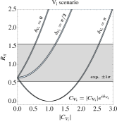
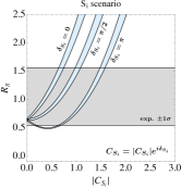
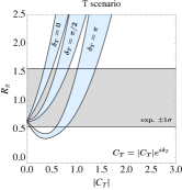
Figure 1: New physics effects on Rπsubscript𝑅𝜋R_{\pi} in the Visubscript𝑉𝑖V_{i}, Sisubscript𝑆𝑖S_{i}, and T𝑇T scenarios. Three values of the complex phase, δX=0subscript𝛿𝑋0\delta_{X}=0, π/2𝜋2\pi/2 and π𝜋\pi, are chosen. The blue regions represent the theoretical predictions on Rπsubscript𝑅𝜋R_{\pi} taking the theoretical uncertainty (±1σplus-or-minus1𝜎\pm 1\sigma) into account. The gray regions show the current experimental bound, Rπexp.1.05±0.51similar-to-or-equalssuperscriptsubscript𝑅𝜋exp.plus-or-minus1.050.51R_{\pi}^{\text{exp.}}\simeq 1.05\pm 0.51.

In Fig. 1, we show Rπsubscript𝑅𝜋R_{\pi} in our new physics scenarios as functions of |CX|subscript𝐶𝑋|C_{X}| for three representative values of the complex phase (defined by CX=|CX|eiδXsubscript𝐶𝑋subscript𝐶𝑋superscript𝑒𝑖subscript𝛿𝑋C_{X}=|C_{X}|e^{i\delta_{X}}) as indicated. The light blue regions are the theoretical predictions with the ±1σplus-or-minus1𝜎\pm 1\sigma uncertainties evaluated with Eqs. (36)-(3.1). The gray region expresses the present experimental bound at the 1σ1𝜎1\sigma level as is estimated in Sec. 1. One finds that the theoretical uncertainty in the vector scenarios is fairly small compared with the experimental error, whereas that in the tensor scenario is significant555The uncertainty in the bottom quark mass, which is fixed in the present work, increases the theoretical uncertainties in the scalar scenarios. Varying mbsubscript𝑚𝑏m_{b} by ±200plus-or-minus200\pm 200 MeV changes at most (Bπτν¯τ)𝐵𝜋𝜏subscript¯𝜈𝜏\mathcal{B}(B\to\pi\tau\bar{\nu}_{\tau}) and (Bτν¯τ)𝐵𝜏subscript¯𝜈𝜏\mathcal{B}(B\to\tau\bar{\nu}_{\tau}) by ±6%plus-or-minuspercent6\pm 6\% and ±7%plus-or-minuspercent7\pm 7\% respectively for |CSi|<1subscript𝐶subscript𝑆𝑖1|C_{S_{i}}|<1. .

One may observe in Eqs. (12), (13) and (34) that 𝒪V1subscript𝒪subscript𝑉1\mathcal{O}_{V_{1}} and 𝒪V2subscript𝒪subscript𝑉2\mathcal{O}_{V_{2}} have the same contribution to Bπτν¯τ𝐵𝜋𝜏subscript¯𝜈𝜏B\to\pi\tau\bar{\nu}_{\tau} whereas their contributions to Bτν¯τ𝐵𝜏subscript¯𝜈𝜏B\to\tau\bar{\nu}_{\tau} posses opposite sign with each other. This is simply because the (axial-)vector current u¯γμb¯𝑢superscript𝛾𝜇𝑏\bar{u}\gamma^{\mu}b (u¯γμγ5b¯𝑢superscript𝛾𝜇superscript𝛾5𝑏\bar{u}\gamma^{\mu}\gamma^{5}b) contributes only to Bπ𝐵𝜋B\to\pi transition (B𝐵B annihilation). Thus, the vector and the axial vector parts of new physics, namely CV=(CV1+CV2)/2subscript𝐶𝑉subscript𝐶subscript𝑉1subscript𝐶subscript𝑉22C_{V}=(C_{V_{1}}+C_{V_{2}})/2 and CA=(CV2CV1)/2subscript𝐶𝐴subscript𝐶subscript𝑉2subscript𝐶subscript𝑉12C_{A}=(C_{V_{2}}-C_{V_{1}})/2 are separately constrained by Bπτν¯τ𝐵𝜋𝜏subscript¯𝜈𝜏B\to\pi\tau\bar{\nu}_{\tau} and Bτν¯τ𝐵𝜏subscript¯𝜈𝜏B\to\tau\bar{\nu}_{\tau} respectively. The same argument applies to 𝒪S1subscript𝒪subscript𝑆1\mathcal{O}_{S_{1}} and 𝒪S2subscript𝒪subscript𝑆2\mathcal{O}_{S_{2}}. The (pseudo)scalar part, CS=(CS1+CS2)/2subscript𝐶𝑆subscript𝐶subscript𝑆1subscript𝐶subscript𝑆22C_{S}=(C_{S_{1}}+C_{S_{2}})/2 (CP=(CS1CS2)/2subscript𝐶𝑃subscript𝐶subscript𝑆1subscript𝐶subscript𝑆22C_{P}=(C_{S_{1}}-C_{S_{2}})/2) is constrained by Bπτν¯τ𝐵𝜋𝜏subscript¯𝜈𝜏B\to\pi\tau\bar{\nu}_{\tau} (Bτν¯τ𝐵𝜏subscript¯𝜈𝜏B\to\tau\bar{\nu}_{\tau}). As stressed above, the tensor operator 𝒪Tsubscript𝒪𝑇\mathcal{O}_{T} contributes only to Bπτν¯τ𝐵𝜋𝜏subscript¯𝜈𝜏B\to\pi\tau\bar{\nu}_{\tau}.

3.2 Present constraints

Refer to caption
Refer to caption
Refer to caption
Refer to caption
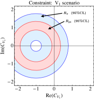
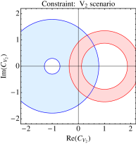
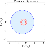
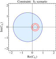
Figure 2: Allowed regions from Rπsubscript𝑅𝜋R_{\pi} and Rpssubscript𝑅psR_{\text{ps}} for V1subscript𝑉1V_{1}, V2subscript𝑉2V_{2}, S1subscript𝑆1S_{1}, and S2subscript𝑆2S_{2} scenarios. The light blue region is allowed from the value of Rπsubscript𝑅𝜋R_{\pi} derived from the Belle experiment at 95% CL, where the theoretical uncertainty is also taken for the evaluation. The light red region is consistent with the experimental value of Rpssubscript𝑅psR_{\text{ps}} taking into account the theoretical uncertainty described in the main text.

The current experimental result for Rπsubscript𝑅𝜋R_{\pi} is given in Sec. 1, Rπexp.1.05±0.51similar-to-or-equalssuperscriptsubscript𝑅𝜋exp.plus-or-minus1.050.51R_{\pi}^{\text{exp.}}\simeq 1.05\pm 0.51. As for Rpssubscript𝑅psR_{\text{ps}}, we obtain Rpsexp.=0.73±0.14superscriptsubscript𝑅psexp.plus-or-minus0.730.14R_{\text{ps}}^{\text{exp.}}=0.73\pm 0.14, while the SM prediction is RpsSM=0.574±0.046superscriptsubscript𝑅psSMplus-or-minus0.5740.046R_{\text{ps}}^{\text{SM}}=0.574\pm 0.046 including the uncertainties of fBsubscript𝑓𝐵f_{B} and f+(q2)subscript𝑓superscript𝑞2f_{+}(q^{2}). Given these experimental data, we present constraints on the Wilson coefficients CXsubscript𝐶𝑋C_{X}’s for V1subscript𝑉1V_{1}, V2subscript𝑉2V_{2}, S1subscript𝑆1S_{1}, and S2subscript𝑆2S_{2} scenarios in Fig. 2, in which the 95% CL allowed regions by Rπsubscript𝑅𝜋R_{\pi} and Rpssubscript𝑅psR_{\text{ps}} for each scenario are shown. The light blue and red regions are allowed by Rπsubscript𝑅𝜋R_{\pi} and Rpssubscript𝑅psR_{\text{ps}}, respectively, taking both the theoretical and experimental uncertainties into account.

The current data of Rπsubscript𝑅𝜋R_{\pi} excludes part of the region of |CX|O(1)similar-tosubscript𝐶𝑋𝑂1|C_{X}|\sim O(1), which is roughly the same order of magnitude as the SM contribution. The excluded region by Rπsubscript𝑅𝜋R_{\pi} does not exceed the one by Rpssubscript𝑅psR_{\text{ps}} in the V1subscript𝑉1V_{1} scenario, but their difference is not so significant. As for the V2subscript𝑉2V_{2} scenario, Rπsubscript𝑅𝜋R_{\pi} and Rpssubscript𝑅psR_{\text{ps}} are complementary because the signs of the new physics contributions relative to the SM ones are opposite in these observables as seen in Eqs. (12), (13) and (34). The S1subscript𝑆1S_{1} and S2subscript𝑆2S_{2} scenarios are constrained more tightly by Rpssubscript𝑅psR_{\text{ps}} because of the chiral enhancement of the pseudoscalar contribution in the purely leptonic decay.
Refer to caption
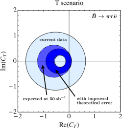
Figure 3: Allowed regions of the tensor scenario for the recent experimental data of Rπsubscript𝑅𝜋R_{\pi} and expected improvements in future. The present allowed region at the 95% CL is depicted in light blue. The (dark) blue region enclosed by the dashed (dotted) curves shows the allowed region expected at SuperKEKB/Belle II with 50ab150superscriptab150\,\text{ab}^{-1} data (and a theoretical uncertainty reduced by a factor of 2).

In Fig. 3, we show the Rπsubscript𝑅𝜋R_{\pi} constraint on CTsubscript𝐶𝑇C_{T}. The light blue region represents the 95% CL allowed region. (The darker blue regions will be explained below.) We see that the present constraint is nontrivial and comparable to the other scenarios even though the theoretical uncertainty are considerably larger. This is because the tensor operator (as normalized in Eq. (3)) tends to give a larger contribution to Rπsubscript𝑅𝜋R_{\pi}. The tensor contribution is expected to be more significant in the BV𝐵𝑉B\to V transitions, such as B¯ρ¯𝐵𝜌\bar{B}\to\rho as in the case of B¯Dτν¯τ¯𝐵superscript𝐷𝜏subscript¯𝜈𝜏\bar{B}\to D^{*}\tau\bar{\nu}_{\tau}.

3.3 Future prospect

From now on, we discuss expected data of the relevant observables at SuperKEKB/Belle II and estimate the possible sensitivity to the new physics scenarios. The current experimental value of Rπsubscript𝑅𝜋R_{\pi} given in Eq. (1) is obtained with 1ab1similar-toabsent1superscriptab1\sim 1\ \text{ab}^{-1} data. We expect 50ab1similar-toabsent50superscriptab1\sim 50\ \text{ab}^{-1} at the SuperKEKB/Belle II experiment. To evaluate the expected sensitivity of Rπsubscript𝑅𝜋R_{\pi} to the new physics scenarios at SuperKEKB/Belle II, we assume that both the statistical and systematic errors in the experiment are reduced with increasing luminosity as 1/11/\sqrt{\mathcal{L}} and that the central value coincides with the SM prediction. Namely, we employ RπBelle II=0.641±0.071superscriptsubscript𝑅𝜋Belle IIplus-or-minus0.6410.071R_{\pi}^{\text{Belle II}}=0.641\pm 0.071. Applying a similar argument to Bτν𝐵𝜏𝜈B\to\tau\nu and Bπν𝐵𝜋𝜈B\to\pi\ell\nu gives RpsBelle II=0.574±0.020superscriptsubscript𝑅psBelle IIplus-or-minus0.5740.020R_{\text{ps}}^{\text{Belle II}}=0.574\pm 0.020666The expected Belle II sensitivity for (Bτν¯)superscript𝐵superscript𝜏¯𝜈\mathcal{B}(B^{-}\to\tau^{-}\bar{\nu}) has been recently studied in Ref. B2sensitivity:Btaunu with Monte-Carlo simulation assuming 0.5ab10.5superscriptab10.5\,\text{ab}^{-1}. Our estimation and their result of the experimental uncertainty scaled to at 50ab150superscriptab150\,\text{ab}^{-1} are consistent. .

Refer to caption
Refer to caption
Refer to caption
Refer to caption
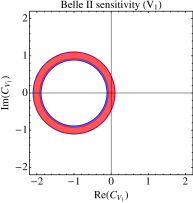
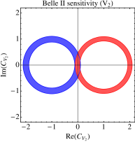
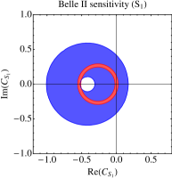
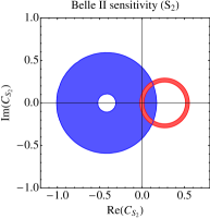
Figure 4: Sensitivity to the new physics scenarios in terms of the 95% CL allowed range of CXsubscript𝐶𝑋C_{X} expected at the SuperKEKB/Belle II with 50ab150superscriptab150\,\text{ab}^{-1} of accumulated data. The “future” experimental data are given as explained in the main text. A new physics contribution for the outside regions of the blue and red colors can be probed by Rπsubscript𝑅𝜋R_{\pi} and Rpssubscript𝑅psR_{\text{ps}}, respectively, at 50ab150superscriptab150\,\text{ab}^{-1} of Belle II.

The 95% CL expected constraints on the Wilson coefficients with these “future” experimental data are shown in Fig. 4 for the V1subscript𝑉1V_{1}, V2subscript𝑉2V_{2}, S1subscript𝑆1S_{1}, and S2subscript𝑆2S_{2} scenarios. A new physics contribution beyond the blue and red regions can be probed by measuring Rπsubscript𝑅𝜋R_{\pi} and Rpssubscript𝑅psR_{\text{ps}}, respectively at Belle II. Each allowed region is annulus-like in the complex plane of CXsubscript𝐶𝑋C_{X}. For the V1subscript𝑉1V_{1} scenario, the new physics sensitivities of Rπsubscript𝑅𝜋R_{\pi} and Rpssubscript𝑅psR_{\text{ps}} are almost degenerate and the region around CV12similar-tosubscript𝐶subscript𝑉12C_{V_{1}}\sim-2 of large negative interference with the SM contribution is allowed by both of them. On the other hand, in the V2subscript𝑉2V_{2} scenario, such regions of CV22similar-tosubscript𝐶subscript𝑉22C_{V_{2}}\sim-2 for Rπsubscript𝑅𝜋R_{\pi} and CV2+2similar-tosubscript𝐶subscript𝑉22C_{V_{2}}\sim+2 for Rpssubscript𝑅psR_{\text{ps}} are incompatible with each other, as is already seen in the current constraint shown in Fig. 2. For the scalar scenarios, the regions of CS1=CS20.8subscript𝐶subscript𝑆1subscript𝐶subscript𝑆2similar-to0.8C_{S_{1}}=C_{S_{2}}\sim-0.8 in Rπsubscript𝑅𝜋R_{\pi} and CS1=CS20.5subscript𝐶subscript𝑆1subscript𝐶subscript𝑆2similar-to0.5C_{S_{1}}=-C_{S_{2}}\sim-0.5 in Rpssubscript𝑅psR_{\text{ps}} are of large negative interference. As is seen in the figures, we can test such a region for the S2subscript𝑆2S_{2} scenario by combining Rπsubscript𝑅𝜋R_{\pi} and Rpssubscript𝑅psR_{\text{ps}} while the sensitivity is relatively weak in the S1subscript𝑆1S_{1} scenario. Therefore, the constraints from Rπsubscript𝑅𝜋R_{\pi} and Rpssubscript𝑅psR_{\text{ps}} are complimentary and measuring both of them at SuperKEKB/Belle II is meaningful to reduce allowed parameter regions, in particular for the V2subscript𝑉2V_{2} and S2subscript𝑆2S_{2} scenarios.

As for the tensor scenario, we also show the expected allowed region for CTsubscript𝐶𝑇C_{T} in Fig. 3. The blue region with the dashed boundary indicates the one that can be tested with 50ab150superscriptab150\,\text{ab}^{-1}, and the darker blue region with the dotted curve corresponds to the result for the case that the theoretical uncertainty in Eq. (3.1) is reduced by a factor of 2. As is explained in Sec. 3.1, the tensor scenario suffers from the larger theoretical uncertainty in Rπsubscript𝑅𝜋R_{\pi} so that we can see the significant effect of the reduction of the theoretical uncertainty. We also find that the present theoretical uncertainties for the vector and scalar scenarios are sufficiently smaller than the future (expected) experimental uncertainties777The reduction of the theoretical error by factor 2, for example, gives only 0.1%percent0.10.1\% and 1%percent11\% differences in the expected allowed regions for the vector and scalar scenarios, respectively. . We note that another observable such as (Bρτν¯)𝐵𝜌𝜏¯𝜈\mathcal{B}(B\to\rho\tau\bar{\nu}) is necessary to exclude the region of large negative interference of CT0.7similar-tosubscript𝐶𝑇0.7C_{T}\sim-0.7.

In Table 1, we present the combined limits of the allowed ranges for CXsubscript𝐶𝑋C_{X} (taken real) in order to quantify the expected sensitivities at SuperKEKB/Belle II. It turns out that, focusing on the vicinity of the origin, the region of |CX|0.03greater-than-or-equivalent-tosubscript𝐶𝑋0.03|C_{X}|\gtrsim 0.03 can be probed in the scalar scenarios. As for the vector and tensor scenarios, the Belle II sensitivity is |CX|0.1similar-tosubscript𝐶𝑋0.1|C_{X}|\sim 0.1.

NP scenario   RπBelle II=0.641±0.071superscriptsubscript𝑅𝜋Belle IIplus-or-minus0.6410.071R_{\pi}^{\text{Belle II}}=0.641\pm 0.071 and RpsBelle II=0.574±0.020superscriptsubscript𝑅psBelle IIplus-or-minus0.5740.020R_{\text{ps}}^{\text{Belle II}}=0.574\pm 0.020   RplBelle II=222±47superscriptsubscript𝑅plBelle IIplus-or-minus22247R_{\text{pl}}^{\text{Belle II}}=222\pm 47
CV1subscript𝐶subscript𝑉1C_{V_{1}} [0.08,0.09];[2.09,1.92]0.080.092.091.92[-0.08,0.09];[-2.09,-1.92] [0.23,0.19];[2.19,1.77]0.230.192.191.77[-0.23,0.19];[-2.19,-1.77]
CV2subscript𝐶subscript𝑉2C_{V_{2}} [0.09,0.08]0.090.08[-0.09,0.08]~{}~{}~{}~{}~{}~{}~{}~{}~{}~{}~{}~{}~{}~{}~{}~{}~{}~{}~{}~{} [0.19,0.23];[1.77,2.19]0.190.231.772.19[-0.19,0.23];~{}~{}~{}~{}~{}[1.77,2.19]
CS1subscript𝐶subscript𝑆1C_{S_{1}} [0.03,0.03];[0.55,0.52]0.030.030.550.52[-0.03,0.03];[-0.55,-0.52] [0.06,0.05];[0.58,0.47]0.060.050.580.47[-0.06,0.05];[-0.58,-0.47]
CS2subscript𝐶subscript𝑆2C_{S_{2}} [0.03,0.03]0.030.03[-0.03,0.03]~{}~{}~{}~{}~{}~{}~{}~{}~{}~{}~{}~{}~{}~{}~{}~{}~{}~{}~{}~{} [0.05,0.06];[0.47,0.58]0.050.060.470.58[-0.05,0.06];~{}~{}~{}~{}~{}[0.47,0.58]
CTsubscript𝐶𝑇C_{T} [0.13,0.10];[1.23,0.56]0.130.101.230.56[-0.13,0.10];[-1.23,-0.56] -
Table 1: Sensitivity to the new physics scenarios in terms of the 95% CL allowed range of CXsubscript𝐶𝑋C_{X} expected at the SuperKEKB/Belle II with 50ab150superscriptab150\,\text{ab}^{-1} of accumulated data. The “future” experimental data are given as explained in the main text. The coefficient CXsubscript𝐶𝑋C_{X} is assumed to be real.

The muonic mode Bμν¯μ𝐵𝜇subscript¯𝜈𝜇B\to\mu\bar{\nu}_{\mu} may also play an important role at SuperKEKB/Belle II. At present, this process has not yet been observed and the current upper limit on the branching ratio is reported as (Bμν¯μ)exp.<1×10⁶superscript𝐵𝜇subscript¯𝜈𝜇exp.1superscript106\mathcal{B}(B\to\mu\bar{\nu}_{\mu})^{\text{exp.}}<1\times 10^{-6} at 90% CL Agashe:2014kda ; Satoyama:2006xn ; Aubert:2009ar . This result may be compared with the SM prediction (Bμν¯μ)SM=(0.41±0.05)×106superscript𝐵𝜇subscript¯𝜈𝜇SMplus-or-minus0.410.05superscript106\mathcal{B}(B\to\mu\bar{\nu}_{\mu})^{\text{SM}}=(0.41\pm 0.05)\times 10^{-6} and thus, we expect that Bμν¯μ𝐵𝜇subscript¯𝜈𝜇B\to\mu\bar{\nu}_{\mu} will be observed with a meaningful statistical significance at SuperKEKB/Belle II. Accordingly, we introduce the pure-leptonic ratio

Rpl=(Bτν¯τ)(Bμν¯μ),subscript𝑅pl𝐵𝜏subscript¯𝜈𝜏𝐵𝜇subscript¯𝜈𝜇\displaystyle R_{\text{pl}}=\frac{\mathcal{B}(B\to\tau\bar{\nu}_{\tau})}{\mathcal{B}(B\to\mu\bar{\nu}_{\mu})}\,, (39)

as we defined Rπsubscript𝑅𝜋R_{\pi}. In this paper, we assume contributions other than the SM do not exist in Bμν¯μ𝐵𝜇subscript¯𝜈𝜇B\to\mu\bar{\nu}_{\mu} as well as Bπν¯𝐵𝜋¯𝜈B\to\pi\ell\bar{\nu}. From the theory side, Rplsubscript𝑅plR_{\text{pl}} is precisely evaluated as

Rpl=mτ2mμ2(1mτ2/mB2)2(1mμ2/mB2)2|1+rNP|2222|1+rNP|2.subscript𝑅plsuperscriptsubscript𝑚𝜏2superscriptsubscript𝑚𝜇2superscript1superscriptsubscript𝑚𝜏2superscriptsubscript𝑚𝐵22superscript1superscriptsubscript𝑚𝜇2superscriptsubscript𝑚𝐵22superscript1subscript𝑟NP2similar-to-or-equals222superscript1subscript𝑟NP2\displaystyle R_{\text{pl}}=\frac{m_{\tau}^{2}}{m_{\mu}^{2}}\frac{(1-m_{\tau}^{2}/m_{B}^{2})^{2}}{(1-m_{\mu}^{2}/m_{B}^{2})^{2}}|1+r_{\text{NP}}|^{2}\simeq 222\,|1+r_{\text{NP}}|^{2}\,. (40)

The dominant source of uncertainty fB|Vub|subscript𝑓𝐵subscript𝑉𝑢𝑏f_{B}|V_{ub}| in the leptonic decay rates cancels out and hence it is free from the |Vub|subscript𝑉𝑢𝑏|V_{ub}| determinations, in which some discrepancies might still remain in the Belle II era.

Following Ref. Satoyama:2006xn , the 1σ1𝜎1\sigma range of the error in (Bμν¯μ)exp.superscript𝐵𝜇subscript¯𝜈𝜇exp.\mathcal{B}(B\to\mu\bar{\nu}_{\mu})^{\text{exp.}} is obtained as ±0.6×10⁶plus-or-minus0.6superscript106\pm 0.6\times 10^{-6} at present. This is expected to be reduced as ±0.08×10⁶plus-or-minus0.08superscript106\pm 0.08\times 10^{-6} with 50ab150superscriptab150\,\text{ab}^{-1} at SuperKEKB/Belle II. Applying the same procedure with Rπsubscript𝑅𝜋R_{\pi}, namely with the expected “future” data being given as RplBelle II=222±47superscriptsubscript𝑅plBelle IIplus-or-minus22247R_{\text{pl}}^{\text{Belle II}}=222\pm 47, we have evaluated the future sensitivity of the ratio Rplsubscript𝑅plR_{\text{pl}} to the new physics scenarios as shown in Table 1. One finds that the sensitivity of Rplsubscript𝑅plR_{\text{pl}} is rather (similar-to\sim factor 2) weaker than that of Rpssubscript𝑅psR_{\text{ps}}. Although Rpssubscript𝑅psR_{\text{ps}} has better performance, the ratio Rplsubscript𝑅plR_{\text{pl}} is still a good observable in the sense that it has the very accurate theoretical prediction and could be used as a consistency check.

4 Summary

We have studied possible new physics in the semi- and pure- tauonic B𝐵B decays, Bπτν¯τ𝐵𝜋𝜏subscript¯𝜈𝜏B\to\pi\tau\bar{\nu}_{\tau} and Bτν¯τ𝐵𝜏subscript¯𝜈𝜏B\to\tau\bar{\nu}_{\tau}, using the model-independent effective Lagrangian including the vector (V1,2subscript𝑉12V_{1,2}), scalar (S1,2subscript𝑆12S_{1,2}), and tensor (T𝑇T) types of interaction. The formulae of the differential branching fractions in the presence of new physics described by the effective Lagrangian are presented with a brief summary of the hadronic form factors in the Bπ𝐵𝜋B\to\pi transition.

We have examined the ratio of the branching fraction of Bπτν¯τ𝐵𝜋𝜏subscript¯𝜈𝜏B\to\pi\tau\bar{\nu}_{\tau} to that of Bπν¯𝐵𝜋subscript¯𝜈B\to\pi\ell\bar{\nu}_{\ell}, Rπsubscript𝑅𝜋R_{\pi} defined in Eq. (2), in order to reduce uncertainties in theoretical calculations in analogy with BD()τν¯τ𝐵superscript𝐷𝜏subscript¯𝜈𝜏B\to D^{(*)}\tau\bar{\nu}_{\tau}. Using the recent results of lattice QCD studies on the relevant form factors, we have evaluated the effects of new physics in Rπsubscript𝑅𝜋R_{\pi} along with its theoretical uncertainty. The theoretical uncertainties in the V1,2subscript𝑉12V_{1,2} scenarios are negligible compared to the present experimental error, and those in the S1,2subscript𝑆12S_{1,2} scenarios are sizable, but sufficiently small. In contrast, the new physics contribution in the T𝑇T scenario is rather uncertain as shown in Fig. 1.

We have obtained the present constraints on the Wilson coefficients that describe possible new physics contributions, CXsubscript𝐶𝑋C_{X} (X=V1,2,S1,2,T𝑋subscript𝑉12subscript𝑆12𝑇X=V_{1,2},S_{1,2},T), comparing the theoretical predictions (with uncertainties mentioned above) of Rπsubscript𝑅𝜋R_{\pi} and Rpssubscript𝑅psR_{\text{ps}} with the experimental data. As shown in Fig. 2, some of regions of |CX|O(1)greater-than-or-equivalent-tosubscript𝐶𝑋𝑂1|C_{X}|\gtrsim O(1) are disfavored by the current data. The sensitivity of Rπsubscript𝑅𝜋R_{\pi} in the V1subscript𝑉1V_{1} scenario is less than that of Rpssubscript𝑅psR_{\text{ps}}, but their difference is not so significant. In the V2subscript𝑉2V_{2} scenario, these two observables probe different regions of CV2subscript𝐶subscript𝑉2C_{V_{2}} and are complementary. As for the S1,2subscript𝑆12S_{1,2} scenarios, Rpssubscript𝑅psR_{\text{ps}} is more sensitive owing to the chiral enhancement. Since the tensor operator does not contribute to Bτν¯τ𝐵𝜏subscript¯𝜈𝜏B\to\tau\bar{\nu}_{\tau}, the T𝑇T scenario is constrained solely by Rπsubscript𝑅𝜋R_{\pi}.

Furthermore, we have discussed the future prospect at the SuperKEKB/Belle II experiment and shown its sensitivity to new physics in terms of expected constraints on CXsubscript𝐶𝑋C_{X}. Assuming that both the statistical and systematic uncertainties in the experiment are reduced as the integrated luminosity is increased to 50ab150superscriptab150\ \text{ab}^{-1} and the central values are given by the SM, we have estimated the expected allowed ranges of CXsubscript𝐶𝑋C_{X} from Rπsubscript𝑅𝜋R_{\pi} and Rpssubscript𝑅psR_{\text{ps}}.

It turns out that the allowed regions of CXsubscript𝐶𝑋C_{X} are significantly reduced in all the scenarios and the region of large negative interference with the SM can be excluded by combining Rπsubscript𝑅𝜋R_{\pi} and Rpssubscript𝑅psR_{\text{ps}} in the V2subscript𝑉2V_{2} and S2subscript𝑆2S_{2} scenarios as shown in Figs. 3 and 4. The SuperKEKB/Belle II experiment can probe the new physics contribution of |CX|subscript𝐶𝑋|C_{X}| as small as 0.030.030.03 in the scalar scenarios and 0.1similar-toabsent0.1\sim 0.1 in the vector and tensor scenarios as seen in Table 1.

Further improvement of sensitivity may be achieved if Rπsubscript𝑅𝜋R_{\pi} and Rplsubscript𝑅plR_{\text{pl}} are measured by a similar method adopted to measure RD()subscript𝑅superscript𝐷R_{D^{(*)}}, namely not separate measurements of the numerator and denominator but direct measurements of the ratios. It is also desired to improve the precision of the tensor form factor as well as to evaluate the scalar form factor by lattice simulation. The latter is useful to eliminate the potential uncertainty in the bottom quark mass arising from the equation of motion. Supplemental observables such as (Bρτν¯)𝐵𝜌𝜏¯𝜈\mathcal{B}(B\to\rho\tau\bar{\nu}) and the q2superscript𝑞2q^{2} distribution of Bπτν¯𝐵𝜋𝜏¯𝜈B\to\pi\tau\bar{\nu} are also helpful to further squeeze CXsubscript𝐶𝑋C_{X} as well as to probe or exclude the region of negative interference in the S1subscript𝑆1S_{1} and T𝑇T scenarios.

Acknowledgment

We are grateful to Florian Bernlochner for his useful comments on the Bπτν¯τ𝐵𝜋𝜏subscript¯𝜈𝜏B\to\pi\tau\bar{\nu}_{\tau} data and Hidenori Fukaya for his suggestion on the lattice QCD result. We also thank Tetsuya Enomoto for discussions in the early stage of this study. This work is supported in part by JSPS KAKENHI Grant Numbers JP25400257 and JP16H03993 (MT), and IBS-R018-D1 (RW).

References

  • (1) J. P. Lees et al., Phys. Rev. Lett., 109, 101802 (2012), arXiv:1205.5442.
  • (2) J. P. Lees et al., Phys. Rev., D88(7), 072012 (2013), arXiv:1303.0571.
  • (3) R. Aaij et al., Phys. Rev. Lett., 115(11), 111803, [Addendum: Phys. Rev. Lett.115,no.15,159901(2015)] (2015), arXiv:1506.08614.
  • (4) M. Huschle et al., Phys. Rev., D92(7), 072014 (2015), arXiv:1507.03233.
  • (5) A. Abdesselam et al. (2016), arXiv:1603.06711.
  • (6) Y. Amhis et al. (2014), arXiv:1412.7515.
  • (7) P. Hamer et al., Phys. Rev., D93(3), 032007 (2016), arXiv:1509.06521.
  • (8) C.-H. Chen and C.-Q. Geng, JHEP, 10, 053 (2006), arXiv:hep-ph/0608166.
  • (9) A. Khodjamirian, Th. Mannel, N. Offen, and Y. M. Wang, Phys. Rev., D83, 094031 (2011), arXiv:1103.2655.
  • (10) F. U. Bernlochner, Phys. Rev., D92(11), 115019 (2015), arXiv:1509.06938.
  • (11) J. A. Bailey et al., Phys. Rev., D92(1), 014024 (2015), arXiv:1503.07839.
  • (12) P. del Amo Sanchez et al., Phys. Rev., D83, 032007 (2011), arXiv:1005.3288.
  • (13) H. Ha et al., Phys. Rev., D83, 071101 (2011), arXiv:1012.0090.
  • (14) J. P. Lees et al., Phys. Rev., D86, 092004 (2012), arXiv:1208.1253.
  • (15) A. Sibidanov et al., Phys. Rev., D88(3), 032005 (2013), arXiv:1306.2781.
  • (16) D. Du et al., Phys. Rev., D93(3), 034005 (2016), arXiv:1510.02349.
  • (17) S. Nandi, S.  K. Patra, and A. Soni (2016), arXiv:1605.07191.
  • (18) C. S. Kim and Ru-Min Wang, Phys. Rev., D77, 094006 (2008), arXiv:0712.2954.
  • (19) M. Tanaka and R. Watanabe, Phys. Rev., D87(3), 034028 (2013), arXiv:1212.1878.
  • (20) R. Dutta, A. Bhol, and A. K. Giri, Phys. Rev., D88(11), 114023 (2013), arXiv:1307.6653.
  • (21) J. A. Bailey et al., Phys. Rev. Lett., 115(15), 152002 (2015), arXiv:1507.01618.
  • (22) C. Bourrely, I. Caprini, and L. Lellouch, Phys. Rev., D79, 013008, [Erratum: Phys. Rev.D82,099902(2010)] (2009), arXiv:0807.2722.
  • (23) C. McNeile, C. T. H. Davies, E. Follana, K. Hornbostel, and G. P. Lepage, Phys. Rev., D85, 031503 (2012), arXiv:1110.4510.
  • (24) A. Bazavov et al., Phys. Rev., D85, 114506 (2012), arXiv:1112.3051.
  • (25) H. Na et al., Phys. Rev., D86, 034506 (2012), arXiv:1202.4914.
  • (26) N. H. Christ et al., Phys. Rev., D91(5), 054502 (2015), arXiv:1404.4670.
  • (27) Y. Aoki et al., Phys. Rev., D91(11), 114505 (2015), arXiv:1406.6192.
  • (28) S. Aoki et al. (2016), arXiv:1607.00299.
  • (29) J. L. Rosner, S. Stone, and R. S. Van de Water, Submitted to: Particle Data Book (2015), arXiv:1509.02220.
  • (30) S. Fajfer, J. F. Kamenik, I. Nisandzic, and J. Zupan, Phys. Rev. Lett., 109, 161801 (2012), arXiv:1206.1872.
  • (31) M. Merola, E. Manoni, and G. De Nardo, Talk at the 4th Belle II Theory Interface Platform (B2TiP) Workshop, Pittsburgh, USA, 23-25 May, https://kds.kek.jp/indico/event/19723/session/40/contribution/75 (2016).
  • (32) K. A. Olive et al., Chin. Phys., C38, 090001 (2014).
  • (33) N. Satoyama et al., Phys. Lett., B647, 67–73 (2007), arXiv:hep-ex/0611045.
  • (34) B. Aubert et al., Phys. Rev., D79, 091101 (2009), arXiv:0903.1220.