Tree-decomposable and Underconstrained Geometric Constraint Problems

Abstract

In this paper, we are concerned with geometric constraint solvers, i.e., with programs that find one or more solutions of a geometric constraint problem. If no solution exists, the solver is expected to announce that no solution has been found. Owing to the complexity, type or difficulty of a constraint problem, it is possible that the solver does not find a solution even though one may exist. Thus, there may be false negatives, but there should never be false positives. Intuitively, the ability to find solutions can be considered a measure of solver’s competence.

We consider static constraint problems and their solvers. We do not consider dynamic constraint solvers, also known as dynamic geometry programs, in which specific geometric elements are moved, interactively or along prescribed trajectories, while continually maintaining all stipulated constraints. However, if we have a solver for static constraint problems that is sufficiently fast and competent, we can build a dynamic geometry program from it by solving the static problem for a sufficiently dense sampling of the trajectory of the moving element(s).

The work we survey has its roots in applications, especially in mechanical computer-aided design (MCAD). The constraint solvers used in MCAD took a quantum leap in the 1990s. These approaches solve a geometric constraint problem by an initial, graph-based structural analysis that extracts generic subproblems and determines how they would combine to form a complete solution. These subproblems are then handed to an algebraic solver that solves the specific instances of the generic subproblems and combines them.

1 Introduction, Concepts and Scope

A geometric constraint problem, also known as a geometric constraint system, consists of a finite set of geometric objects, such as points, lines, circles, planes, spheres, etc., and constraints upon them, such as incidence, distance, tangency, and so on. A solution of a geometric constraint problem P is a coordinate assignment for each of the geometric objects of P that places them in relation to each other such that all constraints of P are satisfied. A problem P may have a unique solution, it may have more than one solution, or it may have no solution.

In this chapter, we are concerned with geometric constraint solvers, i.e., with programs that find one or more solutions of a geometric constraint problem. If no solution exists, the solver is expected to announce that no solution has been found. Owing to the complexity, type or difficulty of a constraint problem, it is possible that the solver does not find a solution even though one may exist. Thus, there may be false negatives, but there should never be false positives. Intuitively, the ability to find solutions can be considered a measure of solver’s competence.

We consider static constraint problems and their solvers. We do not consider dynamic constraint solvers, also known as dynamic geometry programs, in which specific geometric elements are moved, interactively or along prescribed trajectories, while continually maintaining all stipulated constraints. However, if we have a solver for static constraint problems that is sufficiently fast and competent, we can build a dynamic geometry program from it by solving the static problem for a sufficiently dense sampling of the trajectory of the moving element(s).

The work we survey has its roots in applications, especially in mechanical computer-aided design (MCAD). The constraint solvers used in MCAD took a quantum leap with the work by Owen [45]. Owen’s algorithm solves a geometric constraint problem by an initial, graph-based structural analysis that extracts generic subproblems and determines how they would combine to form a complete solution. These subproblems are then handed to an algebraic solver that solves the specific instances of the generic subproblems and combines them. Owen’s graph analysis is top down. A bottom-up analysis was proposed in [3]. Subsequent work expanded the knowledge of

1. the structure and properties of the constraint graph, see Section 3;

2. the geometric vocabulary, see Section 4;

3. the understanding of spatial constraint systems, see Section 5.

We also look briefly at under-constrained problems in Section 6.

Restricted to points and distances, the constraint graph analysis has deep roots in mathematics and combinatorics; see, e.g., [42, 16, 37] for some of these connections. Here, we limit the discussion to constraint problems that are motivated by MCAD applications, and that means that the geometric vocabulary has to be richer than points and distances between them. In the remainder of this section we introduce informally major concepts and methods for solving geometric constraint systems (GCS) with an application perspective in mind.

Note in particular that some definitions in this section may be provisional. Those definitions, although formally incorrect, are so given nevertheless because they facilitate understanding the material. They are clearly identified along with examples that show where they fall short — and what can be done about it.

1.1 Geometric Constraint Systems (GCS)

Fix the space in which to consider a geometric constraint system (GCS). Typical examples are the Euclidean space in 2 or 3 dimensions. Each object to be placed by a GCS instance in that space has a specific number of degrees of freedom (dof), i.e., a specific number of independent coordinates. In Euclidean 2-space, points and lines each have 2 dof. In Euclidean 3-space, a point has 3 dof and a line has 4. A constraint on such objects corresponds to one or more equations expressing the constraints on the coordinates. So, requiring a distance $d$ between two points $A=(A_{x},A_{y})$ and $B=(B_{x},B_{y})$ in 2-space would be expressed by

$$(A_{x}-B_{x})^{2}+(A_{y}-B_{y})^{2}=d^{2}$$

Requiring that the two points are coincident would entail two equations:

$$\begin{array}[]{rcl}A_{x}&=&B_{x}\\ A_{y}&=&B_{y}\end{array}$$

Accordingly, a GCS can be viewed simply as a system of equations: A solution of the GCS, if one exists, is a valuation of the variables, the coordinates, that satisfies all equations. Viewed in this foundational way, solving a GCS boils down to formulating a system of equations in the coordinates of the geometric entities and solving the system by any means appropriate. The equations are almost always algebraic.

1.2 Constraint Graph, Deficit, and Generic Solvability

The approach of treating a GCS as an (unstructured) system of equations is inefficient and almost always unnecessary. Given a GCS, we analyze the structure of the corresponding equation system, and seek to identify smaller subsystems that can be solved independently and that admit especially efficient solution algorithms. Triangle decomposable systems, the main subject of this chapter, do this by analyzing a constraint graph that mirrors the equation structure. The constraint graph is recursively broken down into subgraphs that correspond to independently solvable subsystems. Once subsystems have been solved, their solutions are combined and expose, in the aggregate, additional subsystems that now can be solved separately. Given the GCS problem $P=(U,F)$, with the set of geometric objects $U$ and constraints $F$ upon them, we define the constraint graph $G(P)$ as follows:

Definition 1.1

Given the GCS $P=(U,F)$, its constraint graph $G=(V,E)$ is a labeled undirected graph whose vertices are the geometric objects in $U$, each labeled with its degrees of freedom. There is an edge $(u,v)$ in $E$ if there is a constraint between the geometric objects $u^{\prime}$ and $v^{\prime}$, corresponding to $u$ and $v$ respectively. The edge is labeled by the number of independent equations corresponding to the constraint between $u^{\prime}$ and $v^{\prime}$.

Example 1.2

Consider the constraint problem of Figure 1 that comprises four points in the plane, labeled $A$ through $D$. A line between two points indicates a distance constraint on the points. Thus there are 5 distance constraints, shown left. The corresponding constraint graph is shown on the right.

  

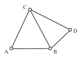
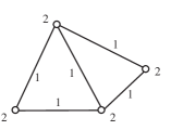
Figure 1: Constraint problem and associated constraint graph.

Since a GCS naturally corresponds to a system of equations, we expect that the number of independent equations should equal the number of variables. The number of independent variables equals the sum of degrees of freedom, i.e., the sum of vertex labels of the constraint graph. Moreover, the number of independent equations equals the sum of the edge labels, in most situations. Thus, we investigate ho the structure of the constraint graph reflects the structure of the equation system that corresponds to the GCS.

As stated, the GCS of Example 1.2 does not prescribe where on the plane to position and orient the points after solving the GCS. Thus, while this GCS is well-constrained, the sum of vertex labels equals the sum of edge labels plus 3. Here, the deficit of 3 corresponds to 3 missing equations that fix where, in the plane, to place the solution. If necessary, the remaining degrees of freedom can be determined by placing the points with respect to a global coordinate system, for example by adding three equations that place $A$ at the origin and $B$ on the (positive) $x$-axis.

So, if the position and orientation of the solution is undetermined, we are assured that a constraint graph where $\sum l(v)-\sum l(e)<3$ in the plane corresponds to an equation system in which at least one equation is not independent. Consequently, we conclude

Definition 1.3

A GCS problem $P$ is generically over-constrained if there is an induced subgraph of the associated constraint graph, such that for the induced subgraph the following holds: $\sum l(v)-\sum l(e)<\kappa$ and none of the constraints fixes the geometric structure with respect to the global coordinate system, where $\kappa=3$ in the plane and $\kappa=6$ in 3-space.

Extrapolating this line of reasoning, we might be led to the conclusion that we can use this structural graph property to define

Definition 1.4

A GCS problem $P$ in the Euclidean plane/space is generically under-constrained if it is not overconstrained and $\sum l(v)-\sum l(e)>\kappa$.

Definition 1.5

(Provisional)
A GCS problem $P$ in the Euclidean plane/space is generically well-constrained if: (i) it is not over-constrained and (ii) the sum of vertex labels of the associated constraint graph equals the sum of the edge labels plus the deficit $\kappa$.

Note, however, for a graph to be well-constrained Definition 1.5 is not sufficient and will be refined in Section 3.7. The problem with Definition 1.5 is best illustrated by an example. The following example exhibits a constraint graph for which the sum of the labels of the vertices equals the sum of the labels of the edges plus $\kappa$ but it contains an overconstrained subgraph and therefore the GCS cannot be well-constrained.

Figure 2: A GCS with an overconstrained and an underconstrained subgraph.

Example 1.6

Consider the constraint graph of Figure 2. For specificity, let the graph vertices be points and the edges distances. The deficit is 3, so it seems that a problem with this constraint graph is well-constrained. Now the subgraph induced by vertices $v_{1},...,v_{4}$ is overconstrained; drop any of the subgraph edges and you obtain a well-constrained subproblem with a deficit 3. On the other hand, the subgraph induced by the vertices $v_{3}...v_{6}$ has a deficit of 4 and is in fact underconstrained; vertices $v_{5}$ and $v_{6}$ cannot be placed. There is an extra constraint in the first subproblem that is not available for the second subproblem.

Even in 2D, dof counting fails to account for well-constrained graphs. We will further study the concept of well-constrained graphs in Section 3.7. Analogously, a GCS in 3-space with deficit 6 that is not overconstrained likewise does not always have a well-constrained graph.

Note that the definitions and properties explained assume in particular that the GCS solution does not have certain symmetries. For instance, consider placing concentrically two circles of given radii. The constraint graph has two vertices, labeled 2 each, and one edge labeled 2, because concentricity implies that the two centers coincide. Here the deficit $\sum l(v)-\sum l(e)$ is 2, less than $\kappa=3$. The system appears to be over-constrained, but the constraint system is well-constrained. The lower deficit reflects the rotational symmetry of the solution.

In the following, we exclude GCS that fix the structure with respect to the coordinate system, as well as GCS that exhibit symmetries that reduce $\kappa$.

1.3 Instance Solvability

Consider constructing a triangle $\triangle(A,B,C)$ with the three sides $a,b,c$ through each of the vertex pairs, in the Euclidean plane. The three points and three lines together have 12 degrees of freedom. Each vertex is incident to two lines, so there are six incidence constraints, each contributing one equation. We add three angle constraints, one for each line pair. The resulting constraint graph has a deficit of three and thus appears to be generically well-constrained. However, the problem is not well-constrained: if the three angle constraints add up to $\pi$, then the GCS is actually underconstrained. If they add up to $\pi/4$, say, the GCS has no solution.

The problem arises from the interdependence of the three angle constraints. Thus generic solvability does not guarantee that problem instances are solvable. In particular, the constraint graph does not record specific dependencies among the equations. Such dependencies often arise from geometry theorems.

Definition 1.7

A GCS is (instance) well-constrained if the associated (algebraic) equation system has one or more discrete real solutions. It is (instance) over-constrained if it has no solution, and is (instance) under-constrained if it has a continuum of solutions.

The definition of generic solvability is fair in the sense that dependencies among some of the constraints, and their equational form, can arise from geometry theorems. The example above is based on a simple theorem, but more complex theorems can arise and may be as hard to detect as solving the equations in the first place.

1.4 Root Identification and Valid Parameter Ranges

Consider Example 1.2. With the distance constraints as drawn, the GCS has multiple solutions, some shown in Figure 3.

     

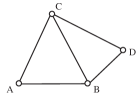
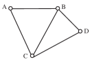
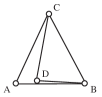
Figure 3: Different solutions of the constraint problem of Example 1.2.

From the equational perspective none is distinguished. From an application perspective usually one is intended. Since the number of distinct solutions can grow exponentially with the number of constrained geometric objects, it is not reasonable to determine all solutions and let the application choose. This application-specific problem is the root identification problem. Some authors use the term chirality.

Solvability generalizes to the determination of valid parameter ranges: It is clear that the distances between the points $A,B,C$, and the distances between the points $B,C,D$ must satisfy the triangle inequality for there to be a (nondegenerate) solution. Considering the metric constraints (distance, angle) as coordinates of points in a configuration space, what is the manifold of points that are associated with solvable GCS instances? Is the manifold connected or are there solutions that cannot be reached from every starting configuration?

1.5 Variational and Serializable Constraint Problems

Some GCS have equation systems that are naturally triangular. That is, intuitively, the geometric objects can be ordered such that they can be placed one-by-one. Such GCS are serializable or sequential constraint problems. GCS that are not serializable have been called variational constraint problems in some of the application-oriented literature. The examples discussed so far are all sequential. The following example shows a variational problem.

Example 1.8

Place 9 points in the plane subject to the 15 distance constraints indicated by the lines, in Figure 4. The following three groups of 4 points each can be placed with respect to each other: $(A,B,C,D)$, $(D,E,F,G)$, and $(G,H,I,A)$. Each of these subproblems is sequential in nature. However, the overall placement problem of all points is not serializable; it is variational.

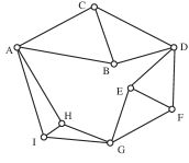
Figure 4: A variational constraint problem.

Serializable constraint problems are of limited expressiveness. Due to their potential efficiency, however, they are used to great effect in some dynamic geometry packages such as Cinderella [6] and GeoGebra [15].

1.6 Triangle-Decomposing Solvers

The overall strategy of triangle-decomposing solvers is to construct the constraint graph and, analyzing the graph, to recursively isolate solvable subproblems. Then, the solved subproblems are recombined. The process is recursive.

For planar constraint systems, triangle-decomposability is understood to be a recursive property in which the base case consists of two vertices (2 dof each) and one edge between them eliminating one of the four dof’s. Larger structures are then solved by isolating three solved structures that pairwise share a single geometric element and thus can be combined by placing the solved structures relative to each other. When this decomposition is done top-down, the solved structures are triconnected; [45]. When the decomposition is done bottom-up, triples of solved components are sought that pairwise share a geometric primitive; [3]. The act of combining such triples has been called a cluster merge.

For the problem of Example 1.8, illustrated in Figure 4, the graph is first decomposed into the three subproblems discussed. Next, each of these subproblems is further broken down. For the subproblem $A,B,C,D$, for example, this might be done by placing, with respect to each other, $A$ and $B$, $B$ and $C$, and $C$ and $A$. Those three subsystems are then combined into the triangle $A,B,C$. This merging step combines three subsystems that pairwise share a point, placing the three shared geometric elements in one geometric construct. The triangle can then be merged with the two subsystems $C$ and $D$, and $B$ and $D$. The result so obtained is the solved subsystem with vertices $A,B,C,D$. Similarly, we solve subproblems $D,E,F,G$ and $G,H,I,A$, each in two merge stpdf. Finally, the entire problem is solved by merging the three subsystem.

The recursion solving the problem of Figure 4 can be thought of either as a top-down decomposition, or as a bottom-up reconstruction.

Note that the top-level merge step places the shared objects, here the points $A$, $D$ and $G$. The distances between these points are not given but can be obtained from the three subproblem solutions. We can think of this process as a plan that is formulated based on the constraint graph analysis. Two questions arise:

1. Since the plan so formulated is not unique, do different decompositions arrive at different solutions? This question is settled by investigating the nature of the recursive decomposition and whether it satisfies a Church-Rosser property.

2. What specific subsystems of equations must be solved and how? This question is approached by analyzing the basic subgraph configurations that can occur, that are allowed by the geometric constraint solver, both when decomposing and when recombining.

Concerning the second question, in our example two key operations are needed: placing two points at a prescribed distance, and placing a third point at a required distance from two fixed points. There is also a third operation that places a rigid geometric configuration $X$ such that two points of $X$ match two given points, using translation and rotation. This operation is used when recombining the three subproblems.

Carrying out these operations entails solving equation systems of a fixed structure. Often, these equation systems are small and can be solved very efficiently. The simplest cases restrict the geometric repertoire to points, lines, and circles of fixed radius. Triangle decomposable systems then require at most solving univariate quadratic polynomials.

More complicated primitives can be added. They include circles of a-priori unknown radius, e.g., [36]; conic sections, e.g., [9]; and Bézier curves, e.g., [19]. Additions impact both the constraint graph analysis as well as the richness of algebraic equation systems that have to be solved. The impact on the graph analysis can be limited to adding additional patterns to cluster merging. So extended, triangle decomposition becomes a more general analysis that can be called tree decomposition. The decomposition remains a tree, but the tree may have different numbers of subtrees associated with a growing repertoire of subgraph patterns. The number of possible patterns is infinite. Therefore, this approach becomes self-limiting. More than that, rigidity no longer has a simple characterization. The contributions to the equation solving algorithms is also considerable. Section 4.3 catalogues what is known about the equation systems required to add just circles of unknown radius.

Because of these rigors, more general techniques have to be considered. For the extended graph analysis, the DR-type algorithms solve the problem by dynamically identifying generically solvable subgraphs; [22, 21]. Likewise, the growth of irreducible algebraic equation systems increasingly motivates searching general equation solvers, including numerical solving techniques, such as Newton iteration, homotopy continuation, and other procedural techniques, for instance [49].

1.7 Scope and Organization

We begin with the graph analysis of triangle-decomposable constraint systems in 2D. These systems play an important role in linkage analysis and graph rigidity, [52, 53, 54]. But even in the Euclidean plane, applications of geometric constraint systems argue for more expressive systems. We can increase expressiveness by enlarging the repertoire of geometric objects, as well as by admitting more complex cluster merging operations.

In the plane, an extended repertoire includes foremost variable-radius circles; that is, circles whose radius is not given explicitly but must be inferred based on the constraints. More advanced objects, such as conics and certain parametric curves, can also be considered. Those additional geometries impact the subsystems of equations that must be solved.

More complex cluster merging operations affect both the constraint graph structures encountered as well as the equation systems that must be solved to position the geometric structures accordingly. We will discuss some examples.

After discussing constraint graphs and generic over-, well-, and under-constrained graphs, we consider the equations that must be solved so as to obtain specific solutions. Here, we explain the structure of those systems as well as some tools to transform the equation systems into simpler ones. Questions of root identification, valid parameter ranges, and order type of solutions are to be discussed. Much is known about these topics in the Euclidean plane. For Euclidean 3-space much less is known. There the equation systems are in general much harder, and the number of cases that should be considered is larger. Even simple sequential problems can require daunting equation systems. A case in point is to find a line in 3-space that is at prescribed distances from four given points, discussed in Section 5.

2 Geometric Constraint Systems

Definition 2.1

A geometric constraint system (GCS) is a pair $(U,F)$ consisting of a finite set $U$ of geometric elements in an ambient space and a finite set $F$ of constraints upon them.

The ambient space typically is $n$-dimensional Euclidean space. The majority of applications require $n=2$ or $n=3$; e.g., [45, 3, 30]. Spherical geometry may also be considered, for instance in nautical applications.

The imposed constraints typically are binary relations. We do not consider higher-order constraints, such as "$C$ be the midpoint between points $A$ and $B$." Note, however, that such constraints can often be expressed by several binary constraints. This can be done in a variety of ways, with or without variable-radius circles.

Definition 2.2

A solution of a geometric constraint system $(U,F)$ is an assignment of coordinates instantiating the elements of $U$ such that the constraints $F$ are all satisfied.

There may be several solutions [10]. Moreover, solutions may or may not be required to be in prescribed position and orientation, in a global coordinate system.

As defined, a GCS is a static problem in that solutions fix the geometric elements with respect to each other. The dynamic geometry problem asks to maintain constraints as some elements move with respect to each other. We consider only static constraint problems and their solvers.

By geometric coverage we understand the diversity of geometric elements admissible in $U$. Points, lines and circles of given radius are adequate for many applications in Euclidean 2-space [45]. For GCS in Euclidean 3-space, an analogous geometric coverage could be points, lines, planes, as well as spheres and cylinders of fixed radii. Here, the number of solutions even of simple GCS can be very large [13].

3 Constraint Graph

The constraint graph of Definition 1.1 is an abstract representation of the equation system equivalent to the geometric constraint problem. The analysis of the graph yields a set of operations used to solve the equations. Ideally, those operations are simple, for instance univariate polynomials of degree 2 [3]. To start the graph analysis, we find minimal constraint problems. That is, constraint problems with a minimal number of geometric objects whose solution defines a local coordinate frame. Such problems depend on ambient space. Consider the following:

Definition 3.1

Given a constraint problem in the Euclidean plane, consisting of two points $A$ and $B$ and a nonzero distance constraint between them. Such a problem is minimal. The associated constraint graph $G=(\{A,B\},\{(A,B)\})$ is a minimal constraint graph.

This minimal constraint problem establishes a coordinate system of the Euclidean plane in which $A$ is the origin and the oriented line $\overrightarrow{AB}$ is the x-axis. This is not the only minimal constraint problem in the plane. Table 1 shows the minimal problems involving the basic geometric objects with 2 dof. Note that fixed-radius circles can be used in lieu of points as long a the centers and points are not coincident. Two parallel lines, at prescribed distance in the plane, are not considered minimal because they do not establish a coordinate frame.

Geoms	Constraint	Notes
Points $A,B$	$d(A,B)$	distance not zero
Point $A$, line $m$	$d(m,A)$	zero distance allowed
Lines $m,n$	$a(m,n)$	lines not parallel

Table 1: Minimal GCS in the Euclidean plane; $d(...)$ denotes distance, $a(...)$ denotes angle.

Table 2 shows the main cases for Euclidean 3-space. In the case of two lines that are skew, a third line $L_{3}$ is constructed that connects the two points of closest approach. Here, $L_{1}$ and $L_{3}$ define a plane that is oriented by $L_{2}$. If the lines $L_{1}$ and $L_{2}$ intersect, they lie on a common plane that is coordinatized by the two lines and is oriented by defining the third coordinate direction using a right-hand rule. If the two lines are parallel, they define a common plane but fail to coordinatize it.

Geoms	Constraint	Notes
Points $p_{1},p_{2},p_{3}$	$d(p_{i},p_{k})$	no zero distance
Point $p$, line $L$	$d(p,L)$	distance not zero
Lines $L_{1},L_{2}$	$d(L_{1},L_{2}),a(L_{1},L_{2})$	lines not parallel
Planes $E_{1},E_{2},E_{3}$	$a(P_{i},P_{k})$	no parallel planes

Table 2: Minimal GCS in Euclidean 3-space; $d(...)$ denotes distance, $a(...)$ denotes angle.

3.1 Geometric Elements and Degrees of Freedom

A geometric element has a characteristic number of degrees of freedom that depends on the type of geometry and the dimensionality of ambient space.

Definition 3.2

Degrees of freedom (dof) are the number of independent, one-dimensional variables by which a geometric object can be instantiated and positioned.

Elementary objects are geometric objects that have a certain number of dof and cannot be decomposed further into more elementary objects. Compound objects can be characterized by a GCS, and consist of one or several elementary objects placed in relation to each other according to a GCS solution instance. A complex object is rigid if its shape cannot change, or, equivalently, if the relative position and orientation of the elementary objects that comprise the complex object cannot change.

The degrees of freedom for elementary geometric objects and for rigid objects in two and three dimensions are summarized in Table 3. Singularities of coordinatization can trigger robustness issues in GCS. Therefore, the representation of elementary geometric objects should be uniform, without singularities. For example, if we represent lines by the familiar $y=mx+b$ formula, lines parallel to the $y$-axis cannot be so represented. This problem can be avoided if we represent a line by its distance from the origin and the direction of the normal vector of the line.

Geom	Geometric Meaning of DoF	2D	3D
Point	Variables representing coordinates	2	3
Line	2D: distance from origin and direction
	3D: distance from origin, direction in 3D	2	4
	direction on the plane
Plane	Distance from origin, direction in 3D		3
Circle, fixed-radius	Coordinates of center, orientation in 3D	2	5
Circle, variable-radius	Coordinates of center, radius, orientation in 3D	3	6
Rigid body	2D: 2 displacements, 1 orientation	3	6
	3D: 3 displacements, 3 orientation
Sphere, fixed- or	3 displacements or	3	4
variable-radius	3 displacements, radius
Ellipse, variable axes	center, axis lengths, axis orientation	5	7
Ellipsoid, variable axes	center, axis lengths, axis orientation		9

Table 3: Degrees of freedom for elementary objects and rigid objects.

Type	Constraint	2D	3D
point-point distance	One equation representing the distance between two points $p_{1},p_{2}$ under the metric $||\ ||$: $||p_{1}-p_{2}||=d$ with $d>0$.	1	1
Angle between lines and planes	Angle between two lines (can be represented by the angle between the normal vectors). Exceptions in 3D: Prallelism between lines eliminates 2DoF. Line-plane orthogonality in eliminates 2 DoF.	1	1
Point on point	For any metric $||p_{1}-p_{2}||=0$ is equivalent to $p_{1}=p_{2}$.	2	3
Point-line distance	One equation expressing the point-line distance.	1	1
Line-line parallel distance	Parallelism and distance.	2	3
Plane-plane parallel distance	Parallelism and distance.	2	3
Point on line	Same as point-line distance In 3D dimension is reduced.	1	2
Line on line	Same as parallel distance between lines in 2D. In 3D an additional DoF is canceled.	2	4
Point on plane	Same as point-plane distance.	-	1
Line on plane	Plane-line parallelism and zero distance.	-	2
Fixing elementary object	Fixing all or some of the DoF of an elementary object.	Dof	DoF

Table 4: Types of constraints and number of dof eliminated.

3.2 Geometric Constraints

Geometric constraints consume one or more dof and are expressed by an equal number of independent equations. A basic set of geometric constraints in the plane is summarized in Table 4. Constraints can be expressed directly. Alternatively, some can be reduced equivalently to other constraints. For example, suppose we stipulate that a circle of radius $r$ be tangent to a line $L$ in the plane. Then we can require equivalently that the center of the circle be at distance $r$ from $L$. For a comprehensive list of constraints involving planes, points and lines in 3D see for example [39, 56]. Finally we should note that distance 0 between two points takes out two degrees of freedom since this causes dimension reduction (from 1-dimensional to 0-dimensional). Similarly, requiring that two lines be parallel at distance $d$ in 3-space eliminates 3 dof, but if $d=0$ the constraint eliminates 4 dof.

3.3 Compound Geometric Elements

Several geometric elements can be conceptually grouped into compound elements. A circular arc is an example. Compound geometric elements are convenient concepts for graphical user interfaces of GCS solvers. Internally, they are decomposed into geometric elements and implied constraints. We illustrate this dual view with the example of a circular arc shown in Figure 5 and explain why it has overall 2 intrinsic parameters.

Since the arc does not have a fixed radius, it lies on a variable-radius circle that has 3 dof. The two end points contribute an additional 4 dof. The two end points are incident to the circle, reducing the overall dof to 5. Position and orientation of the arc, in some coordinate system, requires 3 dof, leaving two intrinsic arc parameters. They can be interpreted as 1 dof for the radius of the arc, and 1 dof for the distance between the end points.

Note that this constraint problem has 4 solutions in general. Orienting the end points, and connecting them with an oriented line, or circle, the arc can be on one of two sides of the directed line. Moreover, the two end points divide the circle into a shorter and a longer arc, in general. Which one is chosen accounts for the other two solutions. Applications require selecting one of these solutions. Several conventions can be followed to determine a unique segment: preservation of the original configuration, preservation of the direction of the curve from the first endpoint towards the second endpoint, the shortest segment and so on.

Figure 5: Building a complex object using one variable radius circle, two end points and two incidence constraints.

3.4 Serializable Graphs

When a GCS is serializable (Section 1.5) the geometric objects can be ordered in such a way that they can be placed sequentially one-by-one as function of preceding, already placed elements. This idea can be formalized as follows.

Definition 3.3

Let $G=(V,E)$ be a GCS graph and $x_{0},x_{1},x_{2}\ldots$ be elements in $V$. We say that $x_{i}$ depends on $x_{k},x_{r},\ldots$, written $x_{i}>x_{k},x_{r},\ldots$, if $x_{i}$ can be placed only after the $x_{k},x_{r},\ldots$ have been placed.

If the constraint graph is serializable, then the pair $(G,>)$ is a directed acyclic graph (DAG) and admits topological sorting [1]. See Example 1.8. More formally,

Definition 3.4

Let $G(V,E)$ be the constraint graph associated with a GCS in Euclidean 2-space. Without loss of generality assume that $G$ is connected. We say that the GCS is serializable if $(G,>)$ describes a sequence of dependencies such that, under a suitable enumeration of $V$,

1. There are elements $x_{0}$ and $x_{1}\in V$ that induce a minimal constraint graph.

2. Each subsequent element $x_{i},~{}~{}~{}2\leq i\leq|V|$ depends on elements $x_{j}$ and $x_{k}$ where $j<i$ and $k<i$.

In general, the enumeration is not unique and depends on the pair $x_{0},x_{1}\in V$ that is placed first. However, as we will see later, different possible sequences derived from a given DAG are equivalent in the sense that they lead to the same final placement for all the objects in $V$ with respect to each other; see Section 3.7.

Example 3.5

Consider the graph in Figure 6(a). The edges have been directed to show dependencies of placement. Choosing $(A,I)$ as starting pair, a valid dependence relation is obtained. The list in Figure 6(b) gives a serial construction based on the graph $(G,>)$.

         

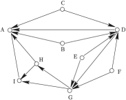
Figure 6: a) DAG derived from a serializable graph, with $(A,I)$ as starting pair. b) A construction sequence respecting the dependencies.

3.5 Variational Graphs

Definition 3.6

A GCS which is not serializable is called variational.

When the GCS is variational, starting with a minimal GCS and applying the dependence relationship to the constraint graph $G=(V,E)$ generates a sequence of dependencies that includes only a subset of elements in $V$. We call it a subsequence and the corresponding subgraph a cluster.

Assuming that the variational GCS is solvable, one repeatedly selects a minimal GCS and applies the dependence relationship, using graph edges not yet used, resulting in a collection of subsequences.

Intuitively, the situation described means that clusters corresponding to different sequences must be merged, usually applying translations and rotations defined by elements shared by subsequences. From an equational point of view, the existence of different subsequences reveals that there are several underlying equations that must be solved simultaneously.

Example 3.7

Figure 7a shows a variational DAG corresponding to the variational constraint problem in Figure 4. We choose three starting pairs $(A,I)$, $(G,F)$ and $(C,B)$. Each allows us to build a DAG from some of the graph vertices and edges. They are listed in Figure 7(b). Notice that each subsequence identifies a serializable subgraph.

  

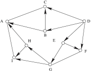
Figure 7: a) DAG derived from the variational graph in Figure 4 with starting pairs $(A,I)$, $(G,F)$ and $(C,B)$. b) Three different subsequences of construction dependencies that can be identified in the DAG.

3.6 Triangle Decomposability

The strategy of triangle-decomposing solvers, as sketched in Section 1, is based on decomposing the constraint graph recursively. Decomposition splits a (sub)graph into 3 (sub)subgraphs that share one vertex pairwise. This is called a triangle decomposition step. More complex splitting configurations can be considered and called tree decomposition. Figure 8 shows a triangle and a more complex tree decomposition step.

                 

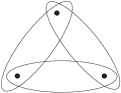
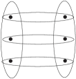
Figure 8: a) Triangle decomposition step. b) More complex tree decomposition step. Split subgraphs are shown as ovals, shared vertices as dots.

From a practical point of view, in the case of GCS in Euclidean 2-space, triangle-decomposable constraint graphs suffice for solving many problems that arise in applications.

We define a triangle decomposition step as follows.

Definition 3.8

Let $G=(V,E)$ be a graph. We say that three subgraphs of $G$, $G_{i}(V_{i},E_{i}),1\leq i\leq 3$, define a triangle decomposition step of $G$ if

1. $V_{1}\cup V_{2}\cup V_{3}=V$, $E_{1}\cup E_{2}\cup E_{3}=E$ and $E_{i}\cap E_{j}=\emptyset,i\neq j$, and

2. There are three vertices, say $u,v,w\in V$, such that $V_{1}\cap V_{2}=\{u\}$, $V_{2}\cap V_{3}=\{v\}$ and $V_{3}\cap V_{1}=\{w\}$.

Example 3.9

Consider the graph $G$ in Figure 7(a). As shown in Figure 9, the subgraphs $G_{1},G_{2}$ and $G_{3}$ define a triangle decomposition step of $G$. Vertices pairwise shared by the subgraphs are $A,D$ and $G$.

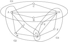
Figure 9: A triangle-decomposition step for the graph shown in Figure 7(a).

Definition 3.10

We say that a ternary tree $T$ is a triangle decomposition for the graph $G$ if

1. The root of $T$ is the graph $G$.

2. Each node of $T$ is a subgraph $G^{\prime}\subset G$ which is either the root of a ternary tree generated by a triangle decomposition step of $G^{\prime}$ or a leaf node with a minimal associated subgraph.

Definition 3.11

A graph for which there is a triangle decomposition is called triangle-decomposable.

In general, a triangle decomposition of a graph is not unique. However, if the graph is triangle decomposable by one sequence of decomposition stpdf, then any legal sequence will decompose the graph [10].

Example 3.12

Consider the graph and the triangle decomposition step shown in Figure 9. Now recursively apply decomposition stpdf to each of the subgraphs $G_{1},G_{2},G_{3}$ until reaching minimal subgraphs. Figure 10 shows two triangle decompositions for the graph considered that differ in the subtree rooted at node $DEFG$. Notice, however, that the set of terminal nodes is the same in both triangle decompositions.

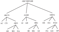
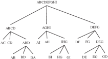
Figure 10: Two different triangle decompositions for the graph shown in Figure 7.

Assume that the three subgraphs $G_{1},G_{2},G_{3}$ are (graphs of) solvable GCS subproblems. Let $u$ and $v$ be the shared vertices of $G_{2}$ and there is no constraint between them. Then $u$ and $v$ constitute a virtual minimal GCS where the constraint relating the two elements is not given but can be deduced from the solution of $G_{2}$. A similar statement can be made about $G_{1}$ and $G_{3}$ and their shared vertices.

The triangle pattern is not the only decomposition construct [3]. Others include the pattern shown in Figure 8b. Intuitively, a decomposition pattern represents an equation system that must be solved simultaneously. Decomposition patterns are infinite in number; see also SECTION 2.2

3.7 Generic Solvability and the Church-Rosser Property

Recall Definitions 3.8, 3.11, and 1.5.

Triangle-decomposable graphs, of GCS in the Euclidean plane, are generically well-constrained, and can be solved either bottom-up [11] or top-down [35]. This assertion is based on the shared geometric elements, of each triangle decomposition step, having 2 dof and being in general position with respect to each other. Variable-radius circles have 3 dof and give rise to a special case illustrated in Figure 11.

             

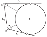
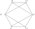
Figure 11: Well-constrained graph with three lines, two points, and a variable-radius circle. a) Constraint problem. Dashed lines represent metric constraints. b) Constraint graph. All vertices have 2 dof except C which has three. Solid lines represent incidence constraints.

Triangle decomposable graphs are also called ternary-decomposable on account of the topology of the decomposition tree. A (recursive) decomposition of a well-constrained triangle decomposable graph is not unique. However, it can be shown using the Church-Rosser property for reduction systems that if one triangle decomposition sequence fully reduces the graph, then all such decompositions must succeed, [10]. The advantage of restricting to triangle-decomposable problems is that a fixed, finite repertoire of algebraic equation systems suffices to solve this class of problems.

Triangle decomposable graphs are a subset of the set of well-constrained constraint graphs of planar GCS. The entire set has been characterized by Laman in [37].

Definition 3.13

Let $G=(V,E)$ be a connected, undirected graph whose vertices represent points in 2D and edges represent distances between points. $G$ is a well-constrained constraint graph of a GCS iff, the deficit of $G$ is 3 and, for every subset $U\subset V$, the induced subgraph $(U,F)$ has a deficit of no less than 3.

Two examples of well-constrained graphs that are not triangle-decomposable are shown in Figure 12.

             

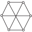
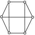
Figure 12: Well-constrained graphs that are not triangle-decomposable. a) Graph $K_{3,3}$. b) Desargue’s graph. All vertices have 2 dof, all edges consume 1 dof.

In triangle decomposition, the irreducible constituents of the constraint graph are the minimal constraint graphs, Definition 3.1. For the general case, the set of irreducible constraint graphs has been characterized in [20] using a network flow approach. Conceptually, irreducible constraint graphs must be solved as a single equation system. Since the graphs can be arbitrarily complex, so can be the equation systems.

    

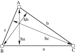
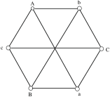
Figure 13: Deriving the geometry of a triangle given its three altitudes. a) Formulating the three altitude problem. b) The resulting constraint graph.

For the planar case, when we have only points and distances the set of triangle decomposable graphs coincides with the set of quadratically solvable graphs. However if we extend to lines and angles, there are quadratically solvable graphs which are not triangle decomposable. Consider the problem of finding a triangle from its three altitudes shown in Figure 13(a). The corresponding graph is shown in Figure 13(b) where the hexagon edges are point-on-line constraints and the diagonals are point-line distance constraints. The geometric problem is quadratically solvable, [31], but the graph, $K_{3,3}$, is not triangle decomposable.

Laman’s theorem holds even if we extend the repertoire of geometries to any geometry having 2 degrees of freedom and the constraints to virtually any constraint of Table 4. However, if we extend the set of geometries to include for example variable radius circles, then the Laman condition is no longer sufficient.

Example 3.14

Consider the GCS of Figure 14. We have two rigid clusters $C_{1}=\{V_{1},V_{2},V_{3},V_{4}\}$ and $C_{2}=\{V_{1},V^{\prime}_{2},V^{\prime}_{3},V^{\prime}_{4}\}$, where $V_{1}$ is a variable-radius circle, $V_{2},V_{3},V^{\prime}_{2},V^{\prime}_{3}$ are points, and $V_{4},V^{\prime}_{4}$ are lines. The constraints $e_{1},e_{2},e^{\prime}_{1},e^{\prime}_{2}$ are distances from the center of $V_{1}$, $e_{6},e^{\prime}_{6}$ are distances from the circumference of $V_{1}$, $e_{5},e^{\prime}_{5}$ are distance constraints, and $e_{3},e_{4},e^{\prime}_{3},e^{\prime}_{4}$ are incidence constraints. The two clusters share the variable-radius circle $V_{1}$.

The graph is clearly a Laman graph but is not rigid, since it is underconstrained — $C_{1}$ and $C_{2}$ can move independently around circle $V_{1}$. The problem is also overconstrained since the radius of $V_{1}$ can be derived independently from cluster $C_{1}$ and from cluster $C_{2}$.

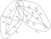
Figure 14: A Laman graph in 2D that is not rigid. V₁ is a variable radius circle. V₂,V₃,V${}^{\prime}_{2}$,V${}^{\prime}_{3}$ are points. V₄, V${}^{\prime}_{4}$ are lines. e₁,e₂,e${}^{\prime}_{1}$,e${}^{\prime}_{2}$ are points. e₃,e₄,e${}^{\prime}_{3}$,e${}^{\prime}_{4}$ are on constraints. e₅, e${}^{\prime}_{5}$ are distances. e₆, e${}^{\prime}_{6}$ are distances from cirlce ( circumference).

3.8 2D and 3D Graphs

Graph analysis for spatial constraint problems is not nearly as mature as the planar case. In the planar case, Definition 3.1 conceptualizes minimal GCS with which a bottom-up graph analysis would start and a top-down analysis would terminate. Table 1 lists the configurations. In 3-space, analogously, the corresponding minimal problem may consist of three points or three planes, with three constraints between them. However, the major configurations shown in Table 2 also include other cases, for example two lines.

In the plane, serially adding one additional point or line requires two constraints. In 3-space, adding a point or plane requires three. The inclusion of lines in 3-space leads to serious complications. For example, since lines have 4 dof, see Table 3, we have to be able to construct lines from given distances from 4 fixed points. Equivalently, we have to construct a common tangent to 4 fixed spheres, a problem known to have up to 12 real solutions, [23]. Work in [62] has explored the optimization of the algebraic complexity of 3D subsystems.

In 3D, the Laman condition is not sufficient. Figure 15 illustrates two hexahedra sharing two vertices. If the length of the edges is given the GCS that arises is also known as the double banana problem. The graph is a Laman graph but the problem corresponds to two rigid bodies (each hexahedron is a rigid body) sharing two vertices and is thus non rigid in the sense that the two rigid bodies are free to rotate around the axis defined by the two shared points. The problem is also clearly overconstrained since the distance of the two shared geometries can be derived independently by each of the two rigid bodies.

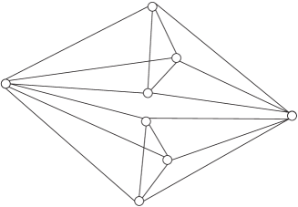
Figure 15: Two hexahedra sharing two points.

A necessary and sufficient condition for rigidity in 3D has been recently presented in [39] for an extended set of geometries and constraints. The authors have extended the theory in [55, 59] to characterize systems of rigid bodies made of points, lines and planes connected by virtually any pairwise constraint (point-point, point-line, line-plane etc) except point-point coincidence. In this approach, a multigraph $(V,(B,A))$ is formulated, where vertices $V$ represent rigid bodies and edges $(B,A)$ stand for primitive constraints that represent single equations between the two 6-vectors that describe the rigid body motion of the two vertices. Primitive constraints intuitively affect at most one degree of freedom. Each geometric constraint is translated to a number of primitive constraints (see Appendix C of [39]). A distinction is made between primitive angular and blind constraints: a primitive angular constraint may affect only a rotational degree of freedom. All other primitive constraints that may affect either a rotational or translational degree of freedom are called blind constraints.

Therefore edges are of two types: angular $(A)$ and blind $(B)$. Such a scheme is minimally rigid if and only if there is a subset $B^{\prime}$ of the blind edges such that (i) $B-B^{\prime}$ is an edge disjoint union of 3 spanning trees and (ii) $A\cup B^{\prime}$ is an edge disjoint union of 3 spanning trees.

Note that this characterization does not capture the cases of Figures 14 and 15. The condition holds for both cases, but rigidity is not guaranteed since they involve point coincidences between rigid bodies directly or indirectly.

4 Solver

After the constraint graph has been analyzed, the implied underlying equations are to be solved. We discuss now how to do that.

4.1 2D Triangle-Decomposable Constraint Problems

We restrict to points and lines in the Euclidean plane. As discussed in Section 3.6, triangle-decomposable constraint systems in the plane require solvers that implement three operations:

1. The two geometric elements of a minimal subgraph (Definition 3.1) are placed consistent with the constraint between them.

2. A third geometric element is placed by two constraints on two geometric elements already placed.

3. Given two geometric elements in fixed position, a rigid-body transformation is done that repositions the two elements elsewhere.

These operations are applied to the decomposition tree, progressing from the leaves of the tree to the root. The solving order is bottom-up regardless whether the decomposition tree was built top-down or bottom-up [45, 10, 3].

Example 4.1

Consider the constraint system of Example 1.2. We choose the subgraph induced by $A$ and $B$ as minimal and place $A$ at the origin and $B$ on the positive $x$-axis, at the stipulated distance from $A$, so executing Operation 1.

We place $C$ by the two constraints on $A$ and $B$, solving at most quadratic, univariate equations, executing Operation 2. The triangle $A,B,C$ is thereby constructed.

Assume that we have solved the triangle $B,C,D$ in like manner, separately and with $B$ and $D$ as vertices of the minimal subgraph. We can now assemble the two triangles by a rigid-body transformation that moves the triangle $B,C,D$ such that the points $B$ and $C$ are matched, using Operation 3.

Note that we can extend the geometric vocabulary of points and lines, adding circles of given radius at no cost. A fixed-radius circle is replaced by its center. A point-on-circle constraint is replaced by a distance constraint between the point and the center, and a tangency constraint by a distance constraint between the tangent and the center.

Operation 1: Minimal GCS Placement

This operation chooses a default coordinate system. There are three pairs of geometric elements that occur in minimal GCS: (point, point), (point, line), and (line, line). The chosen placements are shown in Table 5. Other choices could be made.

$d(p_{1},p_{2})$	Set $p_{1}=(0,0)$, $p_{2}=(d,0)$
$d(p,L)$	Place $L$ on the $x$-axis, $p=(0,d)$
$a(L_{1},L_{2})$	Place $L_{1}$ on the $x$-axis, $L_{2}$ through the origin at angle $a$

Table 5: Placing minimal GCS: $p$ represents points, $L$ represents lines, $d$ distance, $a$ angle.

Operation 2: Constructing one Element from two Constraints

Two elements $A$ and $B$ are given, a third element $C$ is to be placed by constraints upon them. There are six cases, with $p$ denoting a point and $L$ denoting a line.

$$\begin{array}[]{rclrclrcl}(p,p)&\rightarrow&p&(p,L)&\rightarrow&p&(L,L)&\rightarrow&p\\ (p,p)&\rightarrow&L&(p,L)&\rightarrow&L&(L,L)&\rightarrow&L\end{array}$$

The sixth case, $(L,L)\rightarrow L$ is underconstrained. See also [3]. We illustrate with the case $(p,p)\rightarrow L$.

Example 4.2

In the case $(p,p)\rightarrow L$ a line should be constructed by respective distance from two points. Consider the two circles with the given points as center and radius equal to the stipulated distance, as shown in Figure 16. Depending on the three distances, there will be 4, 2 or no real solution in general.

Order the points $A$ and $B$, and orient the circles centered at those points counter-clockwise. Orient the line to be constructed so that the projection of $A$ onto the line precedes the projection of $B$. Then we can distinguish the up to four tangents in a coordinate-independent way: observe whether the line orientation is consistent with the circle orientation (+), or whether the orientations are opposite (–). See also [3].

The degenerate cases where the two circles are tangent to each other yield three solutions or one. In theses cases there is one double solution that represents the coincidence of two solutions, with orientations (+,–) and (–,+), or with orientations (+,+) and (–,–).

     

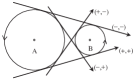
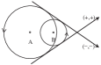
Figure 16: Constructing a line at specific distances from two points. Equivalently, finding common tangents of two circles with radius equal to the stipulated distances. The degenerate cases of 1 or 3 solutions are not shown.

Operation 3: Matching two Elements

The operation requires that the geometric elements to be matched be congruent. The operation is a rigid-body transformation and is routine.

4.2 Root Identification and Order Type

We noted that constructing one element from two constraints can have multiple solutions. As a result, a well constrained GCS has in general an exponential number of solution instances. We shall illustrate this with the simple construction $(p,p)\rightarrow p$.

Example 4.3

Consider placing $n$ points, by $2n-3$ distance constraints between them, and assume that the distance constraints are such that we can place the points by sequentially applying the construction $(p,p)\rightarrow p$. In general, each new point can be placed in two different locations: Let $P_{i}$ and $P_{j}$ be known points from which the new point $Q$ is to be placed, at distance $d_{i}$ and $d_{j}$, respectively. Draw two circles, one about $P_{i}$ with radius $d_{i}$, the other about $P_{j}$ with radius $d_{j}$ as shown in Figure 17. The intersection of the two circles are the possible locations of $Q$. For $n$ points, therefore, we could have up to $2^{n-2}$ solution instances.

Figure 17: Placing one point $Q$ from two points $P_{i},P_{j}$ already known.

Note that not all construction paths derive real solutions. If, in Example 4.3, the distance between $P_{i}$ and $P_{j}$ is larger than the sum of $d_{i}$ and $d_{j}$, then there is no real solution for placing $Q$ and therefore any subsequent construction using this instance of $Q$ is not feasible. Therefore, one might argue that this pruning may result in polynomial algorithms. However, this is unlikely since the problem of determining whether a well constrained GCS has a real solution has been shown to be NP-complete [11].

In general, an application will require one specific solution, usually known as the intended solution. To identify it is not always a trivial undertaking. In [3] finding the intended solution is called the Root Identification Problem. Notice that, on a technical level, selecting the intended solution corresponds to selecting one among a number of different roots of a system of nonlinear algebraic equations.

A well constrained GCS would not necessarily include enough information to identify which solution is the intended one. Consider the following example.

Example 4.4

The well constrained GCS in Figure 18a consists of four points, four straight segments, four point-point distances and an angle. The solution includes four instances. Two correspond to the one shown in Figure 18b and to a symmetric arrangement of the same shape. Solution instances in Figures 18c and 18d are structurally different.

        

Figure 18: a) GCS consisting of four points, four straight segments, four point-point distances and an angle. b),c) and d) Three different solution instances to the GCS.

Clearly, the GCS sketch in Figure 18a does not include any hint on which solution instance must be chosen to be displayed on the user’s screen. Thus, additional information must be supplied to the solver. In [3], approaches applied to overcome this issue have been classified into five categories: Selectively moving geometric elements, adding extra constraints to narrow down the number of possible solution instances, placement heuristics, a dialogue with the constraint solver that identifies interactively the intended solution, and applying a design paradigm approach based on structuring the GCS hierarchically. Next we elaborate on each category.

Moving selected geometry

In this approach, a solution is presented graphically to the user. The user selects, again graphically, certain geometric elements that are considered misplaced. The user then moves those elements where they should be placed in relation to other elements. This approach is used by the DCM solver, [7, 45].

Adding extra constraints

Adding a set of extra constraints to narrow down which is the intended solution instance is an intuitive and simple approach to solving the root identification problem. Extra constraints could capture domain knowledge from the application or could be just geometric — and actually over-specify the GCS. Unfortunately, both ideas result in NP-complete problems [3]. Nevertheless, extra constraints along with genetic algorithms have been applied to solve the root identification problem showing a promising potential. Authors in [60] argue that the approach is both effective and efficient in search spaces with up to $2^{100}$ solution instances. A different application of genetic algorithms to solve the root identification problem is described in [4]. The approach mixes a genetic algorithm with a chaos optimization method.

Example 4.5

Genetic algorithms described in [32, 40, 47], use extra geometric and topological constraints defined as logical predicates on oriented geometries. For example, assume that the polygon in Figure 18a is oriented counterclockwise. The solution shown in Figure 18c would be selected as the intended one by requiring the following two predicates to be fulfilled

$$PointOnSide(P_{3},\stackrel{{\scriptstyle\longrightarrow}}{{P_{1}P_{2}}},left),\qquad Chirality(\stackrel{{\scriptstyle\longrightarrow}}{{P_{2}P_{3}}},\stackrel{{\scriptstyle\longrightarrow}}{{P_{3}P_{4}}},cw)$$

Order-based heuristics

All solvers known to us derive information from the initial GCS sketch and use it to select a specific solution. This is reasonable, because one can expect that a user sketch is similar to what is intended. For instance, by observing on which side of an oriented line a specific point lies in the input sketch it is often appropriate to select solutions that preserve this sidedness. The solver described in [3] seeks to preserve the sidedness of the geometric elements in each construction step: the orientation of three points with respect to each other, of two lines and one point, and of one line and two points. The work described in [3] implements an additional heuristic for arc tangency which aims at preserving the type of tangency present in the sketch. See Figure 20. When the rules fail, the solver opens a dialogue to allow the user to amend the rules as the situation might require. These heuristics are also applied in the solver described in [33].

Example 4.6

Consider placing three points, $P_{1}$, $P_{2}$ and $P_{3}$, relative to each other. The points have been drawn in the initial sketch in the position shown in Figure 19a. The order defined by the points can be determined as follows. Determine where $P_{3}$ lies with respect to the line $\stackrel{{\scriptstyle\longrightarrow}}{{P_{1}P_{2}}}$. If $P_{3}$ is on the line, then determine whether it lies between $P_{1}$ and $P_{2}$, preceding $P_{1}$ or following $P_{2}$. The solver will preserve this orientation if possible. For this example, the solver will choose the point $P_{3}$ as shown in Figure 19b.

                 

Figure 19: Placing three points, $P_{1}$, $P_{2}$ and $P_{3}$, relative to each other. a) Points placed in the initial sketch and induced orientation. b) $P_{3}$ and $P^{\prime}_{3}$ are two possible placements for the third point. Preserving the orientation defined in the sketch leads to select $P_{3}$ as the intended placement.

  

Figure 20: Tangency types. a) Arc and segment tangency. b) Circle-circle tangency.

Dialog with the solver

A useful paradigm for user-solver interaction has to be intuitive and must account for the fact that most application users will not be intimately knowledgeable about the technical working of the solver. So, we need a simple but effective communication paradigm by which the user can interact with the solver and direct it to a different solution, or even browse through a subset of solutions in case the one shown in the user’s screen is not the intended one.

Example 4.7

SolBCN, a ruler-and-compass solver described in [33] offers a simple user-solver interaction tool. Figures 21a and b respectively show the GCS sketch input by the user and the solution instance selected by the heuristic rules implemented. Then, the user can trigger the solution selector by clicking on a button and a list with the set of construction stpdf where a quadratic equation must be solved is displayed, Figure 21c. The user can then change the square root sign for each of these construction stpdf by either selecting it directly or navigating with the next/previous pair of buttons. Figure 21d shows a solution different from the first one so obtained.

        

                 

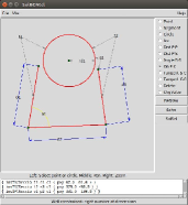
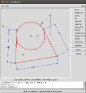
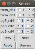
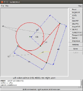
Figure 21: User-solver dialog offered by the ruler-and-compass solver described in [33]. a) GCS sketch. b) Solution instance selected by the heuristics implemented in the solver. c) Solution instance selector. d) Solution instance displayed after changing the square root signs of some construction stpdf.

Navigating the GCS solution space using the approach illustrated in the Example 4.7 is simple. But it has obvious drawbacks. On the one hand, the number of items in the list selector grows exponentially with the number of quadratic construction stpdf in the GCS. On the other hand it is difficult to anticipate how choosing a root sign for a construction step will affect the solution selected by the next sign chosen by the user.

These problems are avoided by considering that, conceptually, all possible solution instances of a GCS can be arranged in a tree whose leaves are the different instances, and whose internal nodes correspond to stages in the placement of individual geometric elements. The different branches from a particular node are the different choices for placing the geometric element. Since the tree has depth proportional to the number of elements in the GCS, stepping from one solution instance to another is proportional to the tree depth only. Moreover, it is possible to define an incremental approach by allowing the user to select at each construction step which tree branch should be used. In solvers based on the DR-planning paradigm, [27], this tree naturally is the construction plan generated by the solver.

Example 4.8

The Equation and Solution Manager [50], features a scalable method to navigate the solution space of GCS. The method incrementally assembles the desired solution to the GCS and avoids combinatorial explosion, by offering the user a visual walk-through of the solution instances to recursively constructed subsystems and by permitting the user to make gradual, adaptive solution choices. Figure 22 illustrates the approach.

  

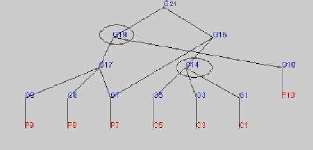
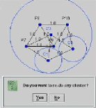
Figure 22: Incremental solution space navigation described in [50]. a) GCS problem including three circles. b) Construction plan graph for the GCS solution. c) GCS solution instance after choosing one of the possible solutions for each construction step. d) A different GCS solution instance after rebuilding the partial construction corresponding to the construction step labeled G14 in the tree.

Design paradigm approach

One of the difficulties in selecting the intended solution of a GCS stems from the fact that geometric elements in a problem sketch are not grouped into logical structures. Authors in [3] argue that hierarchically structuring the constraint problem would alleviate the complexity of solving the root identification problem, for example grouping geometric elements as design features. First a basic, dimension-driven sketch would be given. Then, subsequent dimension-driven stpdf would modify the basic sketch and add complexity. By doing so, the design intent would become more evident and some of the technical problems would be simplified.

Example 4.9

Consider solving the GCS in Figure 23a. The role of the arc is clearly to round the adjacent segments, and thus it is most likely that the solution shown in Figure 23b is the one the user meant rather than the one in Figure 23c, when changing the angles to $30^{\circ}$. However, the solver would be unaware of the intended meaning of the arc. Instead, the user could sketch first the quadrilateral without the arc, and then add the arc to round a vertex. When changing some of the dimensional constraints, the role of the arc would remain that of a round, so preserving the user intent.

    

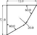
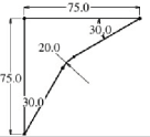
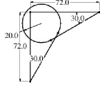
Figure 23: Solution selection by the design paradigm approach: Panel (a) shows the final GCS, panels (b) and (c) two different solution instances. If the arc is introduced as a rounding feature of a constrained quadrilateral, then selecting solution (b) over solution (c) is a logical choice.

4.3 Extended Geometric Vocabulary

So far we discussed 2D constraint solvers that use only points and lines, as well as circles of given radii. Now we will add other geometric element types. This has implications for both the equation solvers as well as for the constraint graph analysis.

The simplest addition allows GCS to include geometric elements of the new type, but only if these elements can be constructed sequentially, from explicit constraints on a set of already placed geometric elements. A more difficult addition would allow the use of elements of the added type in the same way as the core vocabulary of points and lines. Note that a new element type can have more than two degrees of freedom.

Variable-Radius Circles

Circles whose radii have not been given explicitly are arguably the most basic extension of the 2D core solver. Variable-radius circles have three degrees of freedom. We consider two ways in which they can arise:

1. A variable-radius circle is to be constructed by a sequential step from three, already placed geometric entities.

2. A variable-radius circle is to be determined in a step analogous to merging three clusters (Definition 3.8) and the circle acts as a cluster.

Note that a variable-radius circle cannot be a shared element in the sense of Definition 3.8. Shared elements have already been constructed; therefore a shared variable-radius circle has already become a fixed-radius circle.

In the following, we consider points to be circles of zero radius. Consequently, there are four ways in which a variable-radius circle can be constructed sequentially. Table 6 summarizes the equation systems.

It is advantageous to convert a line-distance constraint into two separate tangency constraints, so simplifying the equations that must be solved. For example, if the sought circle $C$ is to be at distance $d$ from line $L$, we work instead with two problems, one in which the circle $C$ is to be tangent to a parallel line $L_{+}$ of $L$. Here $L_{+}$ is at distance $d$ from $L$, on one side of $L$. In the other problem, $C$ is to be tangent to a parallel line $L_{-}$ also at distance $d$, but on the other side of $L$. Analogously, perimeter distance from a given circle reduces to tangency with a circle whose radius has been increased or reduced by said distance.

When deriving the algebraic equations, we work with cyclographic maps, orienting both lines and circles. Briefly, an oriented circle $C$ is mapped to a normal cone $\mu(C)$, with an axis parallel to the $z$-axis and a half angle of $\pi/4$. The cone intersects the $xy$-plane in $C$. Depending on the orientation, the apex of the cone is above or below the $xy$-plane. Considered as zero-radius circle, the point $P$ in the $xy$-plane maps to the normal cone $\mu(P)$ with apex in the $xy$-plane. Oriented lines $L$ in the $xy$-plane are mapped to planes through $L$ at an angle of $\pi/4$ with the $xy$-plane. This reformulates the constraint problem as a spatial intersection problem of planes and cones. See [46, 18, 25, 24, 5] for details and further reading.

The intersection of two normal cones is a conic, in affine space, plus a shared circle at infinity. The conic lies in a plane whose equation is readily obtained by subtracting the two cone equations: if $K_{1}=0$ and $K_{2}=0$ are the two normal cones, then $K_{1}-K_{2}=0$ is the plane that contains the conic in which the two cones intersect.

Example 4.10

Consider the sequential construction problem of finding a circle that is tangent to three given circles. This is the classical Apollonius problem that has eight solutions in general.

We orient the circles and require that the sought circle be oriented consistently with the given circles at the points of tangency. After orienting the given circles, we can map the problem to the intersection, in 3-space, of three normal cones, $C_{1}$, $C_{2}$, and $C_{3}$, each arising from an oriented circle. Intersect two cone pairs, say $C_{1}\cap C_{2}$ and $C_{1}\cap C_{3}$, obtaining two planes that, in turn, intersect in a line $L$ in 3-space. Then intersect $L$ with one of the cones, say $C_{2}$. Two points are obtained that, understood as the apex of a normal cone, map each to one (oriented) circle in the plane that is a solution; see [48]. Algebraically, the solution is obtained by solving linear equations plus one univariate quadratic equation.

There are 8 ways to orient the three circles, but they correspond pairwise, so only four such problems must be solved. If one or more circles are points, they must be considered oriented both ways. So, for each zero-radius circle, the number of solutions reduces by a factor of 2. The special cases of the Apollonius problem have been mapped out and solved in [48] using cyclographic maps.

Given	Equation	Notes
Elements	System
$LLL$	(1,1)	intersect two angle bisectors
$LLC$	(1,2)	intersect two planes and a cone
$LCC$	(1,1,2)	intersect two planes and a cone
$CCC$	(1,1,2)	Apollonius problem; Example 4.10

Table 6: Sequential construction of variable-radius circles. All constraints are tangent constraints. Equations formulated using cyclographic maps. For the cases $LCC$ and $CCC$ the linear equation(s) are from intersecting two cones.

Now consider the determination of variable-radius circles in a cluster merge. Here, there are two constraints from each cluster to the variable-radius circle to be constructed, and the two clusters share a geometric element. The situation is analogous to the triangle merge characterized in Definition 3.8. The various cases and how to solve them have been studied and solved in [25, 24, 5]. Specifically, [25, 24] map out the cases in which the constraints are on the perimeter of the variable-radius circle; and [5] considers constraints on the center of the variable-radius circle as well.

Table 7 and 8 summarize the results from those papers. The approach is conceptually as follows. Let $S_{1}=\{E_{0},E_{1},E_{2}\}$ and $S_{2}=\{E_{0},E_{3},E_{4}\}$ be the clusters constraining the variable-radius circle. The two clusters share element $E_{0}$, either a line denoted $L$, or a circle denoted $C$. The clusters can move relative to each other, translating along the shared line if $E_{0}=L$, or rotating about the center of the shared circle if $E_{0}=C$. Elements $E_{1}$ and $E_{2}$ belong to $S_{1}$ and constrain the sought circle. Likewise, $E_{3}$ and $E_{4}$ are the constraining elements of $S_{2}$. Proceed as follows:

1. Fix the cluster $S_{1}$ that has the more difficult constraining elements $E_{1}$ and $E_{2}$; i.e., the cluster with the larger number of circles.

2. Choose a convenient coordinate system: the shared line $E_{0}=L$ as the $x$-axis, or the origin as the center of the shared circle if $E_{0}=C$.

3. Construct the cyclographic map of all constraining elements. The cones and planes of $S_{2}$ are parameterized by the distance $d$ between $S_{1}$ and $S_{2}$, or else by the angle $\theta$ between $S_{1}$ and $S_{2}$.

4. Construct three planes from the constraining elements $E_{1},\ldots,E_{4}$. They are either cyclographic maps of lines, or normal cone intersections. The elements of $S_{2}$ give rise to parameterized coefficients, by distance $d$ for translation along the $x$-axis, or by angle $\theta$ for rotation around the origin, of the moving cluster $S_{2}$. Intersect the planes, so obtaining a point with parameterized coordinates.

5. Substitute the parameterized point into the equation of the element $E_{1}$ of the fixed cluster, so obtaining a univariate polynomial that finds the intersection point(s) of the four cyclographic objects; a polynomial in $d$ or $\theta$.

6. Solve the polynomial as described, each obtained by a particular configuration of orientations.

Constraint type	Planes	Polynomial degree
$E(LL,LL)$	$[L_{2}],~{}[L_{3}]^{t},~{}[L_{4}]^{t}$	(1,2)
$E(CL,LL)$	$[L_{2}],~{}[L_{3}]^{t},~{}[L_{4}]^{t}$	(2,4)
$E(CL,CL)$	$[L_{2}],~{}[L_{4}]^{t},~{}([C_{1}],[C_{3}]^{t})$	(4,4)
$E(CC,LL)$	$([C_{1}],[C_{2}]),~{}[L_{3}]^{t},~{}[L_{4}]^{t}$	(2,4)
	$([C_{1}],[C_{2}])$
$E(CC,CL)$	$([C_{1}],[C_{3}]^{t})$	(4,4)
	$[L_{4}]$
	$([C_{1}],[C_{2}])$
$E(CC,CC)$	$([C_{1}],[C_{3}]^{t})$	(4,4)
	$([C_{3}],[C_{4}])^{t}$

Table 7: Cluster cases; all constraints on circle perimeter. $E(...)$ denotes whether clusters share a line $L$, the translational case, or share a circle $C$, rotational case. $[X]$ denotes the cyclographic map equation $\mu(X)$ of $X$; $[X]^{t}$ denotes the equation with coefficients parameterized by distance $t$ (translation case) or by angle $\theta$ (rotation case). $(X,Y)$ denotes the intersection plane equation of $X$ and $Y$. The parameterized point is substituted into the equation $[C_{1}]$, except for the first case where it is substituted into $[L_{1}]$. $(m,n)$ denotes the equation degrees, namely $m$ for the translation case $E=L$, and $n$ for the rotation case $E=C$.

Some of the constraints can be on the center $c$ of the variable-radius circle, and [5] considers those cases. Note that there can be at most two constraints on the center of the variable-radius circle, for otherwise the relative position of $S_{2}$ to $S_{1}$ would be determined and the role of the variable-radius circle would be curtailed.

The problem is again solved in the same conceptual manner, but with a twist. When a constraint is placed on the center $c$ of the variable-radius circle, the constraint can be expressed by extending cyclographic maps with a map $\tau(X)$. Here, $\tau(L)$ is a vertical plane through the line $L$. Moreover, $\tau(C)$ is a cylinder through the circle $C$ with axis parallel to the $z$-axis. The results so obtain are summarized in Table 8.

A problem is denoted $E_{0}(E_{1}E_{2},E_{3}E_{4})$. $E_{0}$ is the shared element by the two clusters, a line $L$ or a circle $C$. $E_{1}$ and $E_{2}$ are the two elements of the fixed cluster constraining the variable-radius circle. $E_{3}$ and $E_{4}$ are the two elements of the moving cluster constraining the variable-radius circle. The numbers (m,n) are the equation degrees when $E_{0}=L$ (m), and $E_{0}=C$ (n). An element $E^{\prime}_{k}$ constrains the center, an element $E$ the circumference, of the variable-radius circle.

One center constraint		Two center constraints
Problem	Degree	Problem	Degree
E(LL,LL’)	(1,2)	E(LL,L’L’)	(1,2)
		E(LL’,LL’)	(1,2)
E(CL,LL’)	(2,4)	E(CL,L’L’)	(2,4)
E(CL’,LL)	(2,4)	E(CL’,LL’)	(2,4)
E(C’L,LL)	(2,4)	E(C’L,LL’)	(2,4)
		E(C’L’,LL)	(2,4)
E(CL,CL’)	(4,4)	E(CL,C’L’)	(4,8)
E(CL,C’L)	(4,16)	E(CL’,CL’)	(4,4)
		E(C’L,CL’)	(4,16)
		E(C’L,C’L)	(4,4)
E(CC,LL’)	(2,4)	E(CC,L’L’)	(2,4)
E(CC’,LL)	(4,4)	E(CC’,LL’)	(4,4)
		E(C’C’,LL)	(2,4)
E(CC,CL’)	(4,4)	E(CC,C’L’)	(4,8)
E(CC,C’L)	(4,32)	E(CC’,CL’)	(8,32)
E(CC’,CL)	(8,32)	E(CC’,C’L)	(8,32)
		E(C’C’,CL)	(4,8)
E(CC,CC’)	(16,64)	E(CC,C’C’)	(2,8)
		E(CC’,CC’)	(16,64)

Table 8: Cluster cases with constraints on the center of the variable-radius circle. $(m,n)$ denotes the equation degree for $E=L$ and $E=C$, respectively. $L^{\prime}$ denotes a constraint between a line and the center of the variable-radius circle; $C^{\prime}$ denotes a constraint between a circle and the center of the variable-radius circle.

5 Spatial Geometric Constraints

Compared to constraint problems in the plane, our knowledge of spatial constraint systems is relatively modest. The constraint graph analysis applies with some notable caveats. For example, Laman’s characterization of rigidity does not apply in 3-space, not even when restricting to points only, and distances between them; see Section 3.8. Furthermore, the subsystems isolated by constraint graph decomposition can be complex, especially if lines are admitted to the geometric vocabulary. We illustrate the latter point with a few examples.

Points and Planes

Points and planes comprise the most elementary vocabulary in spatial constraint solving. Both have three degrees of freedom and are dual of each other. In analogy to the minimal constraint graph in 2D (Definition 3.1), a minimal constraint graph in 3D consists of three elements, points or planes, and three constraints, forming a triangle. The initial placement for the four combinations places the elements in canonical order, planes first, points second. Table 9 summarizes the method, [8]. Note that the constraint between two planes is an angle, and the constraint between two points or a point and a plane is a distance. The initial placement fails for the exceptional angles $0$ and $\pi$, as well as for distance 0 between two points.

Canonical Placement of three Points or Planes
	$P_{1}$ placed as the plane $z=0$
$P_{1},P_{2},P_{3}$	$P_{2}$ placed to intersect $P_{1}$ in the $y$-axis
	$P_{3}$ placed to contain the origin
	$P_{1}$ placed as the plane $z=0$
$P_{1},P_{2},p_{3}$	$P_{2}$ placed to intersect $P_{1}$ in the $y$-axis
	$p_{3}$ is placed on the $xz$-plane
	$P_{1}$ placed as the plane $z=0$
$P_{1},p_{2},p_{3}$	$p_{2}$ is placed on the positive $z$-axis
	$p_{3}$ is placed on the $xz$-plane with $z\geq 0$
	$p_{1}$ is placed at the origin
$p_{1},p_{2},p_{3}$	$p_{2}$ is placed on the positive $x$-axis
	$p_{3}$ is placed on the $xz$-plane with $z\geq 0$

Table 9: Placement of three entities that are mutually constrained. $P$ denotes a plane $p$ a point.

Sequential constructions of points and planes are straightforward. The locus of a third point $p$, at respective distances from two known points $p_{1}$ and $p_{2}$, is the intersection of two spheres centered at $p_{1}$ and $p_{2}$. It is a circle that is contained in a plane perpendicular to the line through $p_{1}$ ad $p_{2}$. As before, this fact can be used to simplify the algebra.

The simplest, nonsequential constraint system is the octahedron, consisting of 6 elements and 12 constraints, [28, 29]. The name derives from the constraint graph that has the topology of the octahedron. There are 7 major configurations according to the number of planes. The configurations with 5 and with 6 planes are structurally underconstrained. Solutions of the octahedron constraint system have been proposed in [28, 29, 43, 8]. The number of distinct solutions is up to 16.

Points, Lines and Planes

A line in 3-space has four degrees of freedom. Usually lines are represented with 6 coordinates, using Plücker coordinates, or with 8, using dual quaternions; e.g., [2]. Consequently, the implicit relationships between the coordinates have to be made explicit by additional equations when solving constraint systems with lines in 3-space.

The sequential construction of lines can be trivial, for instance determining a line by distance from two intersecting planes. But it can also be hard, for instance, when determining a line by distance from four given points in space. The latter problem, in geometric terms, asks for common tangents to four fixed spheres. This problem has up to 12 real solutions. The upper bound of 12 was shown in [30] using elementary algebra. The lower bound of 12 was established in [41] with an example. In contrast to the restricted problem of only points and planes, this sequential constraint problem involving lines is therefore much more demanding.

We can constrain two lines by distance from each other, by angle, and also by both distance and angle. Small constraint configurations that involve lines have been investigated, [14, 13]. The papers show that there are 2 variational configurations of 4 lines. They are shown in Figure 24. The papers also show that the number of configurations with 5 geometric elements, including lines, is 17. Moreover, when 6 elements are considered, the number of distinct configurations grows to 683. Because of this daunting growth pattern, it is natural to seek alternatives. One such alternative has been proposed in [58, 57] where, instead of lines, only segments of lines are allowed. Consequently, many constraints can be formulated as constraints on end points. Note that in many applications this is perfectly adequate.

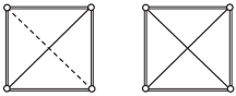
Figure 24: The two variational constraint problems with 4 lines. The 4 double lines represent both angle and distance, the solid diagonals distance, and the dashed diagonal angle constraints.

6 Under-constrained Geometric Constraint Problems

In general, existing geometric constraint solving techniques have been developed under the assumption that problems are well-constrained, that is, they adhere to Definition 1.5 given in Section 1. Put differently, the number of constraints and their placement on the geometric elements define a problem with a finite number of solution instances for non-degenerate configurations. However, there are a number of scenarios where the assumption of well-constrained does not apply. Examples are early stages of the design process when only a few parameters are fixed or in cooperative design systems where different activities in product design and manufacture examine different subsets of the information in the design model, [26]. The problem then is under-constrained, that is, there are infinitely many solution instances for non-degenerate configurations.

Example 6.1

Consider the hook of a car trunk locker shown in Figure 25. Once distances $d_{1}$ and $d_{2}$ have placed the center of the exterior circle of the hook with respect to the hook’s axis of rotation, the designer is mainly interested in finding a value for the angle $\alpha$ where the exterior circle is tangent to the small circle transitioning to the inner circle of the hook. The angle $\alpha$ has to be such that the hook smoothly rotates while closing and opening the hood. At this design stage, the stem shape of the hook is irrelevant.

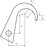
Figure 25: Hook of a car trunk locker.

This, and other simple examples taken from Computer-Aided Design, illustrate the need for efficient and reliable techniques to deal with under-constrained systems. The same need is found in other fields where geometric constraint solving plays a central role, such as kinematics, dynamic geometry, robotics, as well as molecular modeling applications.

Recent work on under-constrained GCS with one degree of freedom, has brought significant progress in understanding and formalizing generically under-constrained systems; [51, 53, 54]. The work focuses on GCS restricted to points and distances, also generically called linkages.

The goal of geometric constraint solving is to effectively determine realizations or embeddings of geometric objects in the ambient space in which the GCS problem is formulated. Thus, the current trend is that solving an under-constrained GCS should be understood as solving some well-constrained GCS derived from the given one.

There are two ways to transform an under-constrained GCS into a well-constrained one: adding to the GCS as many extra constraints as needed or removing from the GCS unconstrained geometric entities. Note that removing constrained entities makes little sense. Accordingly, the literature on under-constrained GCS advocates to transform an under-constrained GCS into a well-constrained one by adding new constraints. This technique was formally defined in [34] as follows.

Definition 6.2

Let $G(V,E)$ be an under-constrained graph associated with a GCS problem. Let $E^{\prime}$ be a set of additional edges each bounded by two distinct vertices in $V$ such that the graph $G^{\prime}(V,E\cup E^{\prime})$ is well-constrained. We say that $E^{\prime}$ is a completion for $G$ and that $G^{\prime}$ is the completed graph of $G$.

Let $\mathcal{G}$ denote the set of geometric constraint graphs. Definitions 1.5, 1.4 and 1.3 given in Section 1 induce in $\mathcal{G}$ a partition as shown in Figure 26. The set of tree-decomposable graphs straddles over the sets of well- and over-constraint graphs. As described in Section 3.6, the set of well-constrained, tree-decomposable graphs are solvable by the tree decomposition approach.

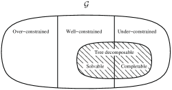
Figure 26: A partition of the geometric constraint graphs set, $\mathcal{G}$. The set of tree-decomposable graphs straddles over the sets of well- and over-constraint graphs.

Within the set of under-constrained graphs we can distinguish two families: Those which are not tree-decomposable and those which are. It is easy to see that there is no completion for a graph in the first family that could transform the graph into a tree-decomposable one. Considering graphs in the second family, Definition 1.5 fixes the number of extra constraints that must be added. However deciding which constraints should actually be added to the graph is not a straightforward matter because the resulting graph could be either over-constrained or well-constrained but not tree-decomposable.

Example 6.3

Figure 27a shows an under-constrained graph. To see that it is tree-decomposable just consider as the first decomposition step the subgraphs induced by the sets of vertices $\{E,F,G\}$, $\{A,G\}$ and $\{A,B,C,D,F\}$. Finding the stpdf needed to complete a tree-decomposition is routine. The completion $E=\{(A,G),(G,B),(G,D),(E,F)\}$ generates the well-constrained graph shown in Figure 27b. To see that the graph is tree-decomposable take as a first decomposition step the two minimal constraint graphs with edges $\{(E,D)\}$ and $\{(E,F)\}$ plus the subgraph induced by edges $\{(A,B),(A,C),(B,C),(B,D),(C,F),(D,F)\}$. However, completion $E=\{(A,E),(E,G),(E,D),(G,D)\}$ results in the graph depicted in Figure 27c which is no tree-decomposable.

                   

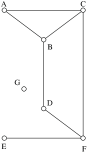
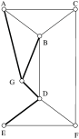
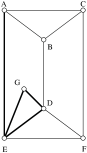
Figure 27: a) An under-constrained, tree-decomposable graph $G$. b) A tree-decomposable completion of $G$. c) A non tree-decomposable completion of $G$.

In what follows we restrict to the completion problem for triangle decomposable GCS.

Definition 6.4

An under-constrained graph $G(V,E)$ is said to be completable if there is a set of edges $E^{\prime}$ which is a completion for $G$.

Notice that completability does not require triangle-decomposability of the underconstrained graph, nor does it imply that a well-constrained, completed graph be tree-decomposable.

Definition 6.5

Let $G(V,E)$ be a triangle-decomposable, under-constrained graph and let $E^{\prime}$ be a completion for $G$. We say that $E^{\prime}$ is a triangle-decomposable completion, (td-completion in short) for $G$ if $G^{\prime}(V,E\cup E^{\prime})$ is triangle-decomposable.

Reported techniques dealing with under-constrained GCS differ mainly in the way they figure out completions as well as whether they aim at figuring out td-completions or just completions. The work in [38] describes an algorithm where the constraint graph is captured as a bipartite connectivity graph whose nodes are either geometric entities or constraints. Each edge connects a constraint node with the constrained geometric node. In analogy to sequential solvers the graph edges are directed to indicate which constraints are used to fix (incident) geometric objects. The connectivity graph is analyzed according to the degrees of freedom of under-constrained geometric nodes. Each under-constrained geometric node is a candidate to support an additional edge to a new constraint, or if there is an edge that heads a propagation path to an existing constraint node that has an unused condition. When there are several candidates on which the new constraint can be established, the selection is left to the user. A similar approach to solve under-constrained GCS based on degrees of freedom analysis is described in [44].

Two different notions of td-completion were introduced in [34]. The first one is called free completion and is computed in three stpdf. First a triangle decomposition for the given graph is figured out. Then the set of under-constrained leaf nodes in the decomposition is identified. Notice that each node in this set stores a subgraph $G(V,E)$ where $|V|=2$ and $E$ is the empty set. Thus one edge is missing. Finally the completion is computed as the set of missing edges in the under-constrained leaf nodes of the triangle-decomposition.

Example 6.6

Figure 28a shows a triangle-decomposition for the under-constrained graph $G(V,E)$ in Figure 27a. We have $|V|=7$ and $|E|=7$. For 2D problems, the general property of a well-constrained graph described in Section 1 is the Laman theorem, [37], $2|V|-|E|=3$. Hence the number of additional edges required to complete $G$ to a well-constrained graph is $|E^{\prime}|=2|V|-|E|-3=4$. The set of leaves in the triangle-decomposition corresponding to under-constrained minimal graphs includes exactly four elements: $\{A,G\},\{B,G\},\{D,E\}$ and $\{D,G\}$. Thus $E^{\prime}=\{(A,G),(B,G),(D,E),(D,G)\}$ is a free completion for $G$. The completed well-constrained graph $G^{\prime}(V,E\cup E^{\prime})$ is shown in Figure 27b.

         

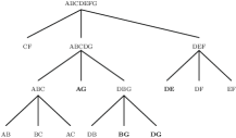
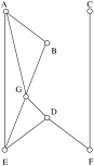
Figure 28: a) A triangle-decomposition for the under-constrained graph $G(V,E)$ in Figure 27a. Pairs of vertices $\{A,G\},\{D,E\},\{B,G\}$ and $\{D,G\}$ in leaf nodes do not define graph edges. b) A set of additional edges defined on $V(G)$. Edges $(A,E),(A,G),(B,G),(D,E),(D,G)$ and $(E,G)$ do not belong to $E$.

The second td-completion is called conditional completion. The first and second stpdf are the same as in the free completion. However, in the third step, edges to complete under-constrained leaf nodes in the decomposition are drawn from an additional graph defined over a subset of vertices of the given graph. If the number of those edges that are not in the original graph is smaller than the number required by Definition 1.5, then the completed graph will remain under-constrained. However a free completion can eventually be applied to get a well-constrained completion.

Example 6.7

Consider again the under-constrained graph $G(V,E)$ in Figure 27a and its triangle-decomposition shown in Figure 28a. The set of under-constrained pairs of vertices in the triangle-decomposition is $\{(A,G),$ $(B,G),$ $(D,E),$ $(D,G)\}$. Assume that the set of additional edges defined on $V(G)$ is

$$\{(A,B),(A,E),(A,G),(B,G),(C,F),(D,F),(E,G),(E,D),(G,D)\}$$

as shown in Figure 28b. Now, additional edges for the completion must be drawn from a set $E^{*}$ such that $E\cap E^{*}=\emptyset$. In the case at hand,

$$E^{*}=\{(A,E),(A,G),(B,G),(D,E),(D,G),(E,G)\}$$

. Thus, a completion for $G(V,E)$ is

$$E^{\prime}=\{(A,G),(B,G),(D,E),(D,G)\}\subset E^{*}$$

. Figure  27b shows the completed graph $G^{\prime}(V,E\cup E^{\prime})$.

A technique to complete general under-constrained graphs is described in [34]. The approach is based on transforming the problem of computing a completion into a combinatorial optimization problem. Edges in the graph and in the additional set are assigned different weights. Then a greedy algorithm generates a well-constrained problem provided that there are enough edges in the additional set. A variant of this approach is reported in [61].

There is a class of 2D, triangle-decomposable, under-constrained GCS that occur in a number of fields like dynamic geometry or mechanical computer aided design. In these GCS the geometries are points, the constraints are usually point-point distances, and exactly one edge is missing in the associated constraint graph. Such GCS are known as linkages.

Example 6.8

Figure 29a shows an illustration of a crankshaft and connecting rod in a reciprocating piston engine. The crankshaft and connecting rod can be abstracted as the GCS shown in Figure 29b. The GCS includes four points $P_{i}$, where $0\leq i\leq 3$, two lines $L_{1},L_{2}$, three point-point distances, $d_{i},0\leq i\leq 2$, one line-line angle, $\alpha$. Moreover, the points $P_{0},P_{2}$ and $P_{3}$ must be on the line $L_{1}$, and the points $P_{0},P_{1}$ must be on the line $L_{2}$. If, for example, values of the distance $d_{1}$ or of the angle $\alpha$ are freely assigned, then the GCS can be considered a linkage.

         

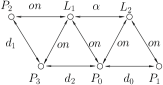
Figure 29: a) A crankshaft and connecting rod in a reciprocating piston engine. b) The crankshaft and connecting rod abstracted as a GCS. c) Geometric constraint graph.

Reachability is an important problem in fields such as dynamic geometry or conformational molecular geometry. It can be formalized as follows:

Let Rs and Re be two realizations of a well defined geometric construction where Rs is called the starting instance and Re the ending instance. Are there continuous transformations that preserve the incidence relationships established in the geometric construction and transform Rs to Re?

The well defined geometric construction in the reachability problem can be understood as a linkage, that is, a well-constrained GCS problem where values assigned to one specific constraint can freely change. In [17] the reachability problem is solved assuming that the underlying GCS is triangle-decomposable. The approach first computes the set of intervals of values that the free constraint can take for which the linkage is realizable. This set of intervals is known as the linkage Cayley configuration space, [12]. When both Rs and Re are realizations with the free constraint taking values within one Cayley interval, the path is an interval arc. When Rs and Re realizations belong to different intervals, finding a path entails figuring out whether there are continuous transitions between consecutive intervals that permit the linkage to reach Re when starting at Rs. If more than one such path is found, one is chosen according to some predefined strategy. In [17] the minimal arc length path is the one chosen.

Example 6.9

The crankshaft and connecting rod GCS in Figure 29b is triangle-decomposable, ruler-and-compass solvable. A construction plan that places each geometric element with respect to each other is

$$\begin{array}[]{llllllll}1.&P_{0}&=&origin()&5.&P_{2}&=&intLC(L_{1},C_{0},s_{1})\\ 2.&P_{3}&=&distPP(P_{0},d_{3})&6.&L_{2}&=&linePA(P_{0},\alpha)\\ 3.&L_{1}&=&line2P(P_{0},P_{3})&7.&C_{1}&=&circleCR(P_{0},d_{0})\\ 4.&C_{0}&=&circleCR(P_{3},d_{1})&8.&P_{1}&=&intLC(L_{2},C_{1},s_{2})\\ \end{array}$$

When a construction step has more than one solution, an orientation parameter is needed to select the desired solution instance. Parameters $s_{1}$ and $s_{2}$ in stpdf 5 and 8 respectively allow to select one of the two points in a line-circle intersection. Figure 30a shows the Cayley configuration space when the point-point distance constraint value $d_{1}$ changes. Intervals labeled $A$, $B$, $C$ and $D$ define orientations and parameter values for which the GCS is realizable. Intervals $A$ and $C$ yield realizations consistent with the one depicted in Figure 30a. Intervals $B$ and $D$ yield realizations where point $P_{2}$ would be placed on the line $L_{1}$ opposite to $P_{1}$ with respect to $P_{0}$. The Cayley configuration space when the varying parameter is the angle $\alpha$ is shown in Figure 30b. Now orientations are represented along a radial axis and angle values for which the solution is realizable are represented as circular intervals.

  

Figure 30: a) Cayley configuration for distance constraint $d_{2}$. b) Cayley configuration for angle constraint $\alpha$.

Linkages are extensively studied in [52, 53, 54]. The object of these works is to lay sound theoretical foundations for a reliable and efficient computation of Cayley configuration spaces for general tree decomposable linkages. New concepts like size and computational complexity are introduced and efficient algorithms are developed to answer a number of questions on linkages like effectively computing Cayley configuration spaces and solving the reachability problem. Methods so far applied to compute Cayley configuration spaces, like the one used in [17], suffer from potential combinatorial growth. The work in [53, 54] shows that for low Cayley complexity GCS problems, computing the configuration space is polynomial in the number of geometric elements of the problem.

Acknowledgement

Hoffmann gratefully acknowledges partial support by the National Science Foundation under award 1361783.

References

- [1] A. Aho, J. Hopcroft, and J. Ullman. The Design and Analysis of Computer Algorithms. Addison-Wesley, 1974.
- [2] W. Blaschke. Kinematik und Quaternionen. VEB Verlag der Wissenschaften, Berlin, Germany, 1960.
- [3] W. Bouma, I. Fudos, C. Hoffmann, J. Cai, and R. Paige. Geometric constraint solver. Computer Aided Design, 27(6):487–501, June 1995.
- [4] C.H. Cao, W. Fu, and W. Li. The research of a new geometric constraint solver. In X.-T Yan, C.-Y Jiang, and N.P. Juster, editors, Perspectives from Europe, and Asia on engineering design and manufacturing, A comparison of engineering design and manufacture in Europe and Asia, pages 205–214. Springer Scinence+Business Media, LLC., 2004.
- [5] C.-S. Chiang and R. Joan-Arinyo. Revisiting variable radius circles in constructive geometric constraint solving. Computer Aided Geometric Design, 221(4):371–399, 2004 2004.
- [6] Cinderella. The interactive geometry software Cinderella, June 2007. http://cinderella.de/tiki-index.php.
- [7] D-Cubed. The Dimensional Constraint Manager. Cambridge, England, 2003. 2D DCM Version 44.0, 3D DCM Version 28.0.
- [8] C. Durand and C. Hoffmann. A systematic framework for solving geometric constraints analytically. JSC, 30:493–519, 2000.
- [9] I. Fudos and C.M. Hoffmann. Constraint-based parametric conics for CAD. Computer Aided Design, 28(2):91–100, 1996.
- [10] I. Fudos and C.M. Hoffmann. Correctness proof of a geometric constraint solver. International Journal of Computational Geometry and Applications, 6(4):405–420, 1996.
- [11] I. Fudos and C.M. Hoffmann. A graph-constructive approach to solving systems of geometric constraints. ACM Transactions on Graphics, 16(2):179–216, April 1997.
- [12] H. Gao and M. Sitharam. Combinatorial classification of 2D underconstrained sytems. In Proceedings of the Seventh Asian Symposium on Computer Mathematics (ASCM 2005), pages 118–127, September 6 2005.
- [13] X.-S. Gao, C. M. Hoffmann, and W. Yang. Solving spatial basic geometric constraint configurations with locus intersection. CAD, 36:111–122, 2004.
- [14] X.-S Gao, C.M. Hoffmann, and W.-Q Yang. Solving spatial basic geometric constraint configurations with locus intersection. In Proceedings of Solid Modeling SM’02, Saarbrucken, Germany, June, 17-21 2002. ACM Press.
- [15] GeoGebra. http://www.geocebra.org/cms, July 2007.
- [16] L. Henneberg. Die graphische Statik der starren Körper. Springer, 1908.
- [17] M. Hidalgo and R. Joan-Arinyo. The reachability problem in constructive geometric constraint solving based dynamic geometry. Journal of Automated Reasoning, 44(7):709–720, 2013. DOI:10.1007/s10817-013-9280-y.
- [18] C. M. Hoffmann. Computer vision, descriptive geometry and classical mechanics. In B. Falcidieno, I. Hermann, and C. Pienovi, editors, Computer Graphics and Mathematics, pages 229–224. Springer Verlag, Eurographics Series, 1992.
- [19] C. M. Hoffmann and J. Peters. Geometric constraints for CAGD. In M. Daehlen, T. Lyche, and L. Schumaker, editors, Mathematical Methods for Curves and Surfaces, pages 237–254. Vanderbilt University Press, 1995.
- [20] Christoph M. Hoffmann, Andrew Lomonosov, and Meera Sitharam. Finding solvable subsets of constraint graphs. In Principles and Practice of Constraint Programming - CP97, Third International Conference, Linz, Austria, October 29 - November 1, 1997, Proceedings, pages 463–477, 1997.
- [21] Christoph M. Hoffmann, Andrew Lomonosov, and Meera Sitharam. Decomposition plans for geometric constraint problems, part ii: new algorithms. Journal of Symbolic Computation, 31(4):409–427, 2001.
- [22] Christoph M. Hoffmann, Andrew Lomonosov, and Meera Sitharam. Decomposition plans for geometric constraint systems, part i: Performance measures for cad. Journal of Symbolic Computation, 31(4):367–408, 2001.
- [23] Christoph M. Hoffmann and Bo Yuan. On spatial constraint solving approaches. In Revised Papers from the Third International Workshop on Automated Deduction in Geometry, ADG ’00, pages 1–15, London, UK, UK, 2001. Springer-Verlag.
- [24] C.M. Hoffmann and C.-S. Chiang. Variable-radius circles of cluster merging in geometric constraints. Part II: Rotational clusters. Computer Aided Design, 34:799–805, October 2002.
- [25] C.M. Hoffmann and C.-X. Chiang. Variable-radius circles of cluster merging in geometric constraints. Part I: Translational clusters. Computer Aided Design, 34:787–797, October 2002.
- [26] C.M. Hoffmann and R. Joan-Arinyo. Distributed maintenance of multiple product views. Computer-Aided Design, 32(7):421–431, June 2000.
- [27] C.M. Hoffmann, A. Lomonosov, and M. Sitharam. Decompostion Plans for Geometric Constraint Systems, Part I: Performance Measurements for CAD. Journal of Symbolic Computation, 31:367–408, 2001.
- [28] C.M. Hoffmann and P.J. Vermeer. Geometric constraint solving in R2 and R3. In D.-Z. Du and F. Hwang, editors, Computing in Euclidean Geometry, pages 266–298. World Scientific Publishing, 1995.
- [29] C.M. Hoffmann and P.J. Vermeer. A spatial constraint problem. In J.P. Merlet and B. Ravani, editors, Computational Kinematics’95, pages 83–92. Kluwer Academic Publ., 1995.
- [30] C.M. Hoffmann and B. Yuan. On spatial constrint solving approaches. In J. Richter-Gebert and D. Wand, editors, Proceedings of ADG’2000, Zurich, Switzerland, 2000.
- [31] R. Joan-Arinyo. Triangles, ruler and compass. Technical Report LSI-95-6-R, Department LiSI, Universitat Politècnica de Catalunya, 1995.
- [32] R. Joan-Arinyo, M.V. Luzón, and A. Soto. Genetic algorithms for root multiselection in constructive geometric constraint solving. Computer & Graphics, 27(1):51–60, 2003.
- [33] R. Joan-Arinyo and A. Soto. A ruler-and-compass geometric constraint solver. In M.J. Pratt, R.D. Sriram, and M.J. Wozny, editors, Product Modeling for Computer Integrated Design and Manufacture, pages 384 – 393. Chapman and Hall, London, 1997.
- [34] R. Joan-Arinyo, A. Soto-Riera, S. Vila-Marta, and J. Vilaplana. Transforming an underconstrained geometric constraint problem into a wellconstrained one. In G. Elber and V.Shapiro, editors, Eight Symposium on Solid Modeling and Applications, pages 33–44, Seattle (WA) USA, June 16-20 2003. ACM Press.
- [35] R. Joan-Arinyo, A. Soto-Riera, S. Vila-Marta, and J. Vilaplana-Pasto. Revisiting decomposition analysis of geometric constraint graphs. In Proceedings of the Seventh ACM Symposium on Solid Modeling and Applications, SMA ’02, pages 105–115, New York, NY, USA, 2002. ACM.
- [36] R.R. Kavasseri. Variable radius circle computations in geometric constraint solving. Master’s thesis, Computyer Sciences. Purdue University, August 1966.
- [37] G Laman. On graphs and the rigidity of plane skeletal structures. J. Engineering Mathematics, 4:331–340, 1970.
- [38] R.S. Latham and A.E. Middleditch. Connectivity analysis: a tool for processing geometric constraints. Computer Aided Design, 28(11):917–928, November 1996.
- [39] Audrey Lee-St.John and Jessica Sidman. Combinatorics and the rigidity of CAD systems. Computer-Aided Design, 45(2):473 – 482, 2013. Solid and Physical Modeling 2012.
- [40] M.V. Luzón, A. Soto, J.F. Gálvez, and R. Joan-Arinyo. Searching the solution space in constructive geometric constraint solving with genetic algorithms. Applied Intelligence, 22:109–124, 2005.
- [41] I. Macdonald, J. Pach, and T. Theobald. Common tangents to four unit balls in R 3. Discrete and Comp. Geometry, 26:1–17, 2001.
- [42] James Clerk Maxwell. On reciprocal figures and diagrams of forces. Philosophical Magazine, 27:250–261, 1864.
- [43] D. Michelucci and S. Foufou. Using the Cayley-Menger determinants for geometric constraint solving. In Solid Modeling and Applications, pages 285–290. ACM, New York, 2004.
- [44] A. Noort, M. Dohem, and W.F. Bronsvoort. Solving over and underconstrained geometric models. In Geometric Constraint Solving. Springer-Verlag, Berlin, Heidelberg, 1998.
- [45] J.C. Owen. Algebraic solution for geometry from dimensional constraints. In R. Rossignac and J. Turner, editors, Symposium on Solid Modeling Foundations and CAD/CAM Applications, pages 397–407, Austin, TX, June 5-7 1991. ACM Press.
- [46] H. Pottmann and M. Peternell. Applications of Laguerre geometry in cagd. CAGD, 15:165–188, 1998.
- [47] E. Yeguas R. Joan-Arinyo, M.V. Luzón. Search space pruning to solve the root identification problem in geometric constraint solving,. Computer-Aided Design and Applications, 6(1):15–25, 2009.
- [48] K. Ramanathan. Variable radius circle computations in geometric constraint solving. Master’s thesis, Department of Computer Science. Purdue University, 1996.
- [49] E. C. Sherbrooke and N. M. Patrikalakis. Computation of the solutions of nonlinear polynomial systems. CAGD, 10:379–405, 1993.
- [50] M. Sitharam, A. Arbree, Y. Zhou, and N. Kohareswaran. Solution space navigation for geometric constraint systems. ACM Transactions on Graphics, 25(2):194–213, April 2006.
- [51] M. Sitharam and H. Gao. Characterizing graphs with convex and connected Cayley configuration spaces. Discrete & Computational Geometry, 43(3):594–625, 2010.
- [52] M. Sitharam and M. Wang. How the beast really moves: Cayley analysis of mechanisms realization spaces using CayMos. Computer Aided Design, 46:205–210, January 2014.
- [53] M. Sitharam, M. Wang, and H. Gao. Cayley configuration spaces of 1-dof tree-decomposable linkages, Part I: Structure and extreme points. arXiv:1112.6008v7[cs.CG], 26 Feb 2014.
- [54] M. Sitharam, M. Wang, and H. Gao. Cayley configuration spaces of 1-dof tree-decomposable linkages, Part II: Combinatorial characterization of complexity. arXiv:1112.6009v4[cs.CG], 7 Nov 2012.
- [55] Tiong-Seng Tay. Rigidity of multi-graphs. i. linking rigid bodies in n-space. Journal of Combinatorial Theory, Series B, 36(1):95 – 112, 1984.
- [56] Gilles Trombettoni and Marta Wilczkowiak. Gpdof — a fast algorithm to decompose under-constrained geometric constraint systems: Application to 3d modeling. International Journal of Computational Geometry and Applications, 16(05n06):479–511, 2006.
- [57] H.A. van der Meiden. Semantics of Families of Objects. PhD thesis, Delft Technical University, 2008.
- [58] H.A. van der Meiden and W.F. Bronsvoort. A constructive approach to calculate parameter ranges for systems of geometric constraints. Computer-Aided Design, 38(4):275–283, 2006.
- [59] Neil White and Walter Whiteley. The algebraic geometry of motions of bar-and-body frameworks. SIAM J. Algebraic Discrete Methods, 8(1):1–32, January 1987.
- [60] E. Yeguas, R. Joan-Arinyo, and M.V. Luzón. Modeling the performance of evolutionary algorithms on the root identification problem: A case study with PBIL and CHC algorithms. Evolutionary Computation, 19(1):107–135, 2011.
- [61] G.-F. Zhang and X.-S Gao. Well-constrained completion and decomposition for under-constrained geometric consraint problems. Int. Jour. of Computational Geometry & Applications, 16(5-6):461–478, 2006.
- [62] Y. Zhou. Combinatorial decomposition, generic independence and algebraic complexity of geometric constraint systems. Applications in biology and engineering. PhD thesis, University of Florida, 2006.