Constraining primordial and gravitational mode coupling with the
position-dependent bispectrum of the large-scale structure

Abstract

We develop and study the position-dependent bispectrum. It is a generalization of the recently proposed position-dependent power spectrum method of measuring the squeezed-limit bispectrum. The position-dependent bispectrum can similarly be used to measure the squeezed-limit trispectrum in which one of the wavelengths is much longer than the other three. In this work, we will mainly consider the case in which the three smaller wavelengths are nearly the same (the equilateral configuration). We use the Fisher information matrix to forecast constraints on bias parameters and the amplitude of primordial trispectra from the position-dependent bispectrum method. We find that the method can constrain the local-type $g_{\rm NL}$ at a level of $\sigma(g_{\rm NL}^{\rm local})\approx 3\times 10^{5}$ for a large volume SPHEREx-like survey; improvements can be expected by including all the triangular configurations of the bispectra rather than just the equilateral configuration. However, the same measurement would also constrain a much larger family of trispectra than local $g_{\rm NL}$ model. We discuss the implications of the forecasted reach of future surveys in terms of super cosmic variance uncertainties from primordial non-Gaussianities.

I Introduction

A key property of any correlation function in the density fluctuations is the degree to which the local statistics can differ from the global statistics due to coupling between local (short wavelength) Fourier modes and background (long wavelength) Fourier modes. For example, the amplitude of the local density power spectrum in sub-volumes of a survey may be correlated with the long-wavelength density mode of the sub-volume Chiang et al. (2014). This observable goes by the name of “position-dependent power spectrum” and is a measure of an integrated bispectrum that gets most of its contribution from the squeezed-limit bispectrum. It is a probe both of non-linear structure formation (such as non-linear gravitational evolution and non-linear bias) and of primordial three-point correlations in the curvature fluctuations. The position-dependent power spectrum is easier to measure than directly measuring the bispectrum, and the position-dependent two-point correlation function has been recently measured from the SDSS-III BOSS data in Chiang et al. (2015).

In this work, we consider the generalization of the position-dependent power spectrum to higher order correlation functions (see also Munshi and Coles (2016)). Given the increasing computational difficulty in directly measuring higher order statistics, studying position-dependent quantities provides a practical route to extract some of the most important information from higher order correlations. In particular, we focus on the position-dependent bispectrum, which is a measure of an integrated trispectrum. Measurements of the galaxy bispectrum have been carried out recently by the SDSS collaboration Gil-Marín et al. (2015a, b).

For simplicity, we will limit this initial analysis to the position dependence in the amplitude of the equilateral configuration of the galaxy bispectrum. We obtain the expected constraints on a large family of primordial trispectra (including $g_{\rm NL}^{\rm local}$, see below) as well as on the linear and quadratic bias parameters using the Fisher information matrix formalism for the proposed SPHEREx (Spectro-Photometer for the History of the Universe, Epoch of Reionization, and Ices Explored) Doré et al. (2014) galaxy survey.

The primordial bispectrum has been well studied, but measurements or constraints of higher order correlations contain independent information. Constraints beyond the bispectrum are limited by the computational difficulty of searching for an arbitrary trispectrum and so far just a few theoretically motivated examples have been studied. One useful case is the “local” model, where the non-Gaussian Bardeen potential field, $\Phi_{\rm NG}(\textbf{x})$, is a non-linear but local function of a Gaussian random field, $\phi_{\rm G}(\textbf{x})$. The standard local “$g_{\rm NL}$” trispectrum is generated by a term proportional to $\phi^{3}_{\rm G}(\textbf{x})$. The Planck mission has constrained the amplitude of this trispectrum $g_{\rm NL}^{\rm local}=(-9.0\pm 7.7)\times 10^{4}\,(1\sigma)$ Ade et al. (2016a). Constraints from SDSS photometric quasars using the scale-dependent bias Dalal et al. (2008) give $|g_{\rm NL}^{\rm local}|\lesssim 2\times 10^{5}$ Leistedt et al. (2014).

The interesting feature of the local ansatz (in the bispectrum, trispectrum and beyond) is the significant coupling between long- and short-wavelength modes of the primordial perturbations. A convincing detection of such a coupling would have two important implications: it would introduce an additional source of cosmic variance in connecting observations to theory Nelson and Shandera (2013); Bramante et al. (2013); LoVerde et al. (2013); Adhikari et al. (2016), and it would rule out the single-clock inflation models Senatore and Zaldarriaga (2012).

While the local ansatz provides a particularly simple example of correlations that couple long- and short-wavelength modes, it is of course not the unique example. Constraining the position dependence of the equilateral configuration of the bispectrum constrains not only $g_{\rm NL}^{\rm local}$, but a large family of other trispectra as well, as we will detail below. In addition, testing for position dependence in the equilateral configuration is particularly interesting because it could signal a deviation from single clock inflation models (since it measures the four-point correlation function) even if the average bispectrum is consistent with the single clock inflation models.

The paper is structured as follows. In the next section we introduce the idea of position-dependent power spectrum and bispectrum. Starting with a review of the position-dependent power spectrum studied in detail in Chiang et al. (2014, 2015), we will discuss and derive expressions for position-dependent bispectrum in terms of the angle-averaged integrated trispectrum. We then present the position-dependent bispectrum from a generic primordial trispectrum, with two illustrative examples (Section III). In Section IV we discuss the galaxy four-point correlation functions from which we measure primordial trispectrum amplitudes, which will be followed by the discussion of the method of the forecast based on Fisher information matrix. We will report and discuss the results of our Fisher forecasts in Section VI, and conclude in Section VII.

II Position-dependent power spectrum and bispectrum

II.1 Position-dependent power spectrum

Consider a full survey volume in which the density fluctuation field $\delta(\textbf{x})$ is defined, and its spherical sub-volumes with a radius $R$ (and volume $V_{R}$) . The smoothed (long-wavelength) density field and the local power spectrum in a sub-volume centered at $\textbf{x}_{R}$ are then given by:

$$\delta(\textbf{k})_{\textbf{x}_{R}} = \int d^{3}\textbf{x}\;\delta(\textbf{x})W_{R}(\textbf{x}-\textbf{x}_{R})e^{-i\textbf{x}\cdot\textbf{k}}$$ (1)

$$= \int\frac{d^{3}\textbf{q}}{(2\pi)^{3}}\;\delta_{\textbf{k}-\textbf{q}}W_{R}(\textbf{q})e^{-i\textbf{x}_{R}\cdot\textbf{q}}$$

$$P(\textbf{k})_{\textbf{x}_{R}} = \frac{1}{V_{R}}\int\frac{d^{3}\textbf{q}_{1}}{(2\pi)^{3}}\;\int\frac{d^{3}\textbf{q}_{2}}{(2\pi)^{3}}\;\delta_{\textbf{k}-\textbf{q}_{1}}\delta_{-\textbf{k}-\textbf{q}_{2}}$$ (2)

$$W_{R}(\textbf{q}_{1})W_{R}(\textbf{q}_{2})e^{-{i}\textbf{x}_{R}\cdot(\textbf{q}_{1}+\textbf{q}_{2})},$$

where $W_{R}(\textbf{q})$ is the Fourier transform of the window function. In this work, we will use the spherical top-hat as the window function, which is defined in real space as:

$$W_{R}(\textbf{x})=\begin{cases}1,{\;\rm if\;|\textbf{x}|\leq R}\\ 0,{\;\rm if\;|\textbf{x}|>R}\end{cases}.$$ (3)

The correlation between the local power spectrum and the long-wavelentgh density contrast in each sub-volume $\left(\bar{\delta}_{\textbf{x}_{R}}=(1/V_{R})\delta(\textbf{k}=0)_{\textbf{x}_{R}}\right)$ gives an integrated bispectrum which is defined as

$$iB_{R}(\textbf{k}) \equiv \langle P(\textbf{k})_{\textbf{x}_{R}}\bar{\delta}_{\textbf{x}_{R}}\rangle$$ (4)

$$= \frac{1}{V_{R}^{2}}\int\frac{d^{3}\textbf{q}_{1}}{(2\pi)^{3}}\int\frac{d^{3}\textbf{q}_{3}}{(2\pi)^{3}}W_{R}(\textbf{q}_{1})W_{R}(-\textbf{q}_{13})$$

$$W_{R}(\textbf{q}_{3})B(\textbf{k}-\textbf{q}_{1},-\textbf{k}+\textbf{q}_{13},-\textbf{q}_{3}),$$

where $\textbf{q}_{13}\equiv\textbf{q}_{1}+\textbf{q}_{3}$. See Chiang et al. (2014) for the details of the derivation. Because the Fourier space window function $W_{R}(\textbf{q})$ drops for $|\textbf{q}|>\pi/R$, for modes well within the sub-volume ($k\gg\pi/R$), the above expression is dominated by the squeezed-limit bispectrum and simplifies to:

$$iB_{R}(\textbf{k})\approx\frac{1}{V_{R}^{2}}\int\frac{d^{3}\textbf{q}}{(2\pi)^{3}}W_{R}^{2}(\textbf{q})B(\textbf{k},-\textbf{k}+\textbf{q},-\textbf{q}),$$ (5)

where we have also used the Fourier transform of the equality $W_{R}^{2}(\textbf{x})=W_{R}(\textbf{x})$ that follows from Eq. (3). The squeezed limit approximation Eq. (5) produces exactly the same result as the squeezed limit of Eq. (4) for any separable bispectrum of the form Chiang et al. (2014)

$$B(\textbf{k}_{1},\textbf{k}_{2},\textbf{k}_{3})=f(k_{1},k_{2},\hat{k}_{1}\cdot\hat{k}_{2})P(k_{1})P(k_{2})+2{\,\rm perm}.$$

Note that this is in general not the case for the integrated trispectrum (Section II.2).

Finally, it is useful to define the reduced integrated bispectrum,

$$ib_{R}(k)=\frac{iB_{R}(k)}{P(k)\sigma_{R}^{2}}.$$ (6)

where $iB_{R}(k)$ now is the angle-averaged integrated bispectrum. Here, and throughout, we assume the statistical isotropy of the Universe and do not include the redshift-space distortion. The reduced integrated bispecturm, in this case, contains all relevant information.

II.2 Position-dependent bispectrum

Building upon the idea of the position-dependent power spectrum, we now divide a survey volume in sub-samples and measure the bispectrum in individual sub-volumes centered on $\textbf{x}_{R}$. This position-dependent bispectrum is given by (note that we have used only two-wavevector arguments below because the third wavevector of the bispectrum is fixed by the triangular condition: $\textbf{k}_{3}=-(\textbf{k}_{1}+\textbf{k}_{2})\equiv-\textbf{k}_{12}$)

$$B(\textbf{k}_{1},\textbf{k}_{2})_{\textbf{x}_{R}}= \frac{1}{V_{R}}\left[\prod_{i=1}^{3}\int\frac{d^{3}\textbf{q}_{i}}{(2\pi)^{3}}W_{R}(\textbf{q}_{i})e^{-{i}\textbf{x}_{R}\cdot\textbf{q}_{i}}\right]$$

$$\qquad\times\delta_{\textbf{k}_{1}-\textbf{q}_{1}}\delta_{\textbf{k}_{2}-\textbf{q}_{2}}\delta_{-\textbf{k}_{12}-\textbf{q}_{3}},$$ (7)

and the correlation of the position-dependent bispectra with the mean overdensities of the sub-volumes is given by an integrated trispectrum as

$$iT(\textbf{k}_{1},\textbf{k}_{2}) \equiv \Big{\langle}B(\textbf{k}_{1},\textbf{k}_{2})_{\textbf{x}_{R}}\bar{\delta}_{\textbf{x}_{R}}\Big{\rangle}$$ (8)

$$= \frac{1}{V_{R}^{2}}\left[\prod_{i=1}^{4}\int\frac{d^{3}\textbf{q}_{i}}{(2\pi)^{3}}W_{R}(\textbf{q}_{i})e^{-{i}\textbf{x}_{R}\cdot\textbf{q}_{i}}\right]$$

$$\qquad\times\Big{\langle}\delta_{\textbf{k}_{1}-\textbf{q}_{1}}\delta_{\textbf{k}_{2}-\textbf{q}_{2}}\delta_{-\textbf{k}_{12}-\textbf{q}_{3}}\delta_{-\textbf{q}_{4}}\Big{\rangle}.$$

The above equation contains the trispectrum $T$ defined as

$$\Big{\langle}\delta_{\textbf{q}_{1}}\delta_{\textbf{q}_{2}}\delta_{\textbf{q}_{3}}\delta_{\textbf{q}_{4}}\Big{\rangle}=(2\pi)^{3}\delta_{D}(\textbf{q}_{1234})T(\textbf{q}_{1},\textbf{q}_{2},\textbf{q}_{3},\textbf{q}_{4}),$$ (9)

and therefore can be re-written as

$$iT(\textbf{k}_{1},\textbf{k}_{2})= \frac{1}{V_{R}^{2}}\left[\prod_{i=1}^{3}\int\frac{d^{3}\textbf{q}_{i}}{(2\pi)^{3}}W_{R}(\textbf{q}_{i})\right]W_{R}(-\textbf{q}_{123})$$

$$\times T(\textbf{k}_{1}-\textbf{q}_{1},\textbf{k}_{2}-\textbf{q}_{2},-\textbf{k}_{12}+\textbf{q}_{123},-\textbf{q}_{3}).$$ (10)

When all modes in the bispectrum are well inside the sub-volume, $|\textbf{k}_{1}|$, $|\textbf{k}_{2}|$, $|\textbf{k}_{12}|\gg\pi/R$, we can use the same approximation as in Section II.1 that the expression is dominated by the squeezed-limit of the trispectrum in which one of the wave-numbers is much smaller than the others,

$$T(\textbf{k}_{1}-\textbf{q}_{1},\textbf{k}_{2}-\textbf{q}_{2},-\textbf{k}_{12}+\textbf{q}_{123},-\textbf{q}_{3})$$ (11)

$$\simeq T(\textbf{k}_{1},\textbf{k}_{2},-\textbf{k}_{12}+\textbf{q}_{3},-\textbf{q}_{3}).$$

With this approximation and the identity $W_{R}^{3}(\textbf{x})=W_{R}(\textbf{x})$, we simplify the integrated trispectrum as

$$iT(\textbf{k}_{1},\textbf{k}_{2})=\frac{1}{V_{R}^{2}}\int\frac{d^{3}\textbf{q}}{(2\pi)^{3}}W_{R}^{2}(\textbf{q})T(\textbf{k}_{1},\textbf{k}_{2},-\textbf{k}_{12}+\textbf{q},-\textbf{q}).$$ (12)

We then define the angle-averaged integrated trispectrum as

$$iT(k_{1},k_{2}) = \int\frac{d^{2}\hat{k}_{1}}{4\pi}\int\frac{d^{2}\hat{k}_{2}}{4\pi}\,iT(\textbf{k}_{1},\textbf{k}_{2})$$

$$= \frac{1}{V_{R}^{2}}\int\frac{q^{2}dq}{2\pi^{2}}W_{R}^{2}(q)$$

$$\times\left[\int\frac{d^{2}\hat{k}_{2}}{4\pi}\int\frac{d^{2}\hat{q}}{4\pi}T(\textbf{k}_{1},\textbf{k}_{2},-\textbf{k}_{12}+\textbf{q},-\textbf{q})\right],$$

where we have removed the $\hat{k}_{1}$ integral by explicitly fixing $\hat{k}_{1}\equiv\hat{z}$.

The integrated trispectrum measures the correlation between the local three-point correlation function (scales smaller than the sub-volume size) and the (long-wavelength) density flustuation on the sub-volume scale. That is, in Fourier space, the integrated trispectrum signal is dominated by the squeezed-limit quadrilateral configurations (of connected four-point function) in which one of the momenta is smaller than the others. Note, however, that unlike that case for the bispectum, the squeezed limit of the trispectrum cannot be defined only with the length of the four momenta. Therefore, strictly speaking, the approximation Eq. (11) works for the trispectrum that depend only on the magnitudes of the four momenta. In this case, the angular integrals in Eq. (10) have no additional contribution and therefore the approximation in Eq. (12) is expected to give exact result in the $q\rightarrow 0$ limit. On the other hand, for generic trispectra which also depend on the length of two diagonals, or the angle between momenta, the approximation may not give the exact result even in the squeezed limit. For example, for the tree-level matter trispectrum $T^{(1)}$ (see Appendix A), we find that the angle-averaged trispectrum from the approximation Eq. (LABEL:eq:angavg) is slightly different from the result of the large-scale structure consistency relations Valageas (2014); Kehagias et al. (2014). The difference, however, is only marginal and does not affect the main result of this paper.

III Position-dependent bispectrum for a primordial trispectrum

As the position-dependent bispectrum depends on the squeezed limit of the trispectrum, its measurement can provide constraints on the primordial non-Gaussianities. In the rest of the paper, we calculate how a primordial trispectrum could generate position dependence in the observed bispectrum, and calculate the projected uncertainty on measuring the primordial trispectrum amplitude by this method. In this section we consider the four-point statistics at the level of initial conditions (and denote the Bardeen potential by $\Phi$), and evolve it linearly. In Section IV, we will work out the corresponding expressions with the galaxy density contrast ($\delta_{g}$) generated from non-linear gravitational evolution and non-linear bias.

III.1 Position dependence from a general primordial trispectrum

We write a general primordial trispectrum by using symmetric kernel functions as follows Baytaş et al. (2015):

$$T_{\Phi}(\textbf{k}_{1},\textbf{k}_{2},\textbf{k}_{3},\textbf{k}_{4})=g_{\rm NL}P_{\Phi}(k_{1})P_{\Phi}(k_{2})P_{\Phi}(k_{3})$$

$$\times N_{3}(\textbf{k}_{1},\textbf{k}_{2},\textbf{k}_{3},\textbf{k}_{4})+({\rm 3\;cyc.})$$ (14)

where the kernel $N_{3}$ is symmetric in the first three momenta (the last momentum is fixed by quadrilateral condition: $\textbf{k}_{4}=-\textbf{k}_{123}$).

The widely studied $g_{\rm NL}^{\rm local}$ model is a very useful benchmark case and corresponds to the simple case of $N_{3}(\textbf{k}_{1},\textbf{k}_{2},\textbf{k}_{3},\textbf{k}_{4})=6$. In the squeezed limit (and for the perfectly scale-invariant primordial power spectrum, $n_{s}=1$), where one of the momenta is much smaller than the other three, the trispectrum scales as

$$T^{g_{\rm NL}^{\rm local}}_{\Phi}(\textbf{k}_{1},\textbf{k}_{2},\textbf{k}_{3},q\rightarrow 0)$$ (15)

$$= \,\frac{3g_{\rm NL}^{\rm local}}{q^{3}}\left[P_{\Phi}(k_{1})P_{\Phi}(k_{2})+({\rm 2\;cyc.})\right]+\mathcal{O}(q^{0}).$$

Notice that the quantity in the square brackets is (up to normalization) the usual local ansatz bispectrum, which peaks on squeezed configurations and is non-zero in the equilateral configuration. The integrated trispectrum in this case is particularly simple:

$$iT_{\Phi}(\textbf{k}_{1},\textbf{k}_{2})^{g_{\rm NL}^{\rm local}}=6g_{\rm NL}^{\rm local}\sigma_{\Phi,R}^{2}\left[P_{\Phi}(k_{1})P_{\Phi}(k_{2})+({\rm 2\;cyc.})\right]$$

where

$$\sigma_{\Phi,R}^{2}=\frac{1}{V_{R}^{2}}\int\frac{d^{3}\textbf{q}}{(2\pi)^{3}}W_{R}^{2}(\textbf{q})P_{\Phi}(q)$$

is the dimensionless, r.m.s. value of the Bardeen’s potential smoothed over the radius $R$. Notice that for small $q$ (modes much larger than the box size), this integral diverges logarithmically (proportional to $\int dq/q$).

It is possible to find trispectra that reduce in the squeezed limit to other bispectral shapes besides the standard local template. For example, Ref. Baytaş et al. (2015) has written down two different examples (Eq.(D3) and Eq.(D5) of that paper) that both have the same squeezed limit

$$T^{g_{\rm NL}^{\rm equil}}_{\Phi} (\textbf{k}_{1},\textbf{k}_{2},\textbf{k}_{3},q\rightarrow 0)=\frac{1}{q^{3}}\Big{[}P_{\Phi}(k_{1})P_{\Phi}(k_{2})$$ (17)

$$\left.\times\left(-6+4\frac{k_{1}+k_{2}}{k_{3}}+2\frac{k_{1}^{2}+k_{2}^{2}}{k_{3}^{2}}-4\frac{k_{1}k_{2}}{k_{3}^{2}}\right)+{\rm 2\;cyc.}\right]$$

$$+\mathcal{O}\left(\frac{1}{q^{2}}\right).$$

Here, the term in square brackets is the equilateral bispectrum, but notice that the strength of coupling to the background, fixed by the scaling as $1/q^{3}$, is the same as that for the local trispectrum.

The two examples generalize to trispectra whose leading order behavior in the squeezed limit can be schematically written as

$$T_{\Phi}(\textbf{k}_{1},\textbf{k}_{2},\textbf{k}_{3},q\rightarrow 0)\propto\frac{1}{q^{3}}\left(\frac{q}{\mathcal{F}(k_{i})}\right)^{\beta}B^{\rm eff}(\textbf{k}_{1},\textbf{k}_{2},\textbf{k}_{3})$$ (18)

where $B^{\rm eff}$ has the properties of a bispectrum and $\mathcal{F}(k_{i})$ is a dimension 1 function of the momenta $\textbf{k}_{1},\textbf{k}_{2},\textbf{k}_{3}$. Comparing with Eq.(15) shows that for a fixed configuration of the bispectrum $B^{\rm eff}$, all trispectra with $\beta=0$ will generate the same average strength of position dependence for that configuration as the $g_{\rm NL}^{\rm local}$ ansatz does.

Note that the position dependent bispectrum $B^{\rm eff}$ from the leading term in the squeezed limit of the trispectrum does not fully characterize the trispectrum. For example, the distinction between the two trispectra in Baytaş et al. (2015) that both generate equilateral bispectra in biased sub-volumes is the doubly-squeezed limit of the trispectra ($\textbf{k}_{4}$, $\textbf{k}_{3}\rightarrow 0$). Namely, one of the two trispectra will also lead to a position-dependent power spectrum whereas the other does not. (This is related to terms that are sub-leading in the position-dependent bispectrum.) So, a distinction between the two can be made by correlating the square of the mean sub-volume overdensities with the power spectra: $\langle P(\textbf{k})_{\textbf{x}_{R}}\bar{\delta}_{\textbf{x}_{R}}^{2}\rangle$. The dominant contribution from matter trispectrum in that case, in the squeezed limit, can be obtained from the $n=2$ response function $R_{2}(k)$ in Wagner et al. (2015). We will further pursue the utility of this quantity in distinguishing the two types of primordial trispectra in a forthcoming publication.

Before specifying to the equilateral configuration that we will use for forecasting in the next section, we use Eq.(14) to derive the position-dependent bispectrum in terms of the kernel that defines a generic trispectrum. Restricting to cases where $\beta\geq 0$ for simplicity, the leading contribution in the squeezed limit ($\textbf{k}_{4}=\textbf{q}\rightarrow 0$) can be expressed as:

$$T_{\Phi}(\textbf{k}_{1},\textbf{k}_{2}, -\textbf{k}_{12}-\textbf{q},\textbf{q})\approx g_{\rm NL}P_{\Phi}(q)P_{\Phi}(k_{1})P_{\Phi}(k_{2})$$ (19)

$$N_{3}(\textbf{q},\textbf{k}_{1},\textbf{k}_{2},-\textbf{k}_{12}-\textbf{q})+({2\,{\rm cyc.}}),$$

where we have used $P_{\Phi}(q)\gg P_{\Phi}(k_{1}),P_{\Phi}(k_{2}),P_{\Phi}(k_{3})$. Now, the integrated trispectrum becomes

$$iT_{\Phi}(\textbf{k}_{1} \textbf{k}_{2})=g_{\rm NL}P_{\Phi}(k_{1})P_{\Phi}(k_{2})$$ , (20)

$$\times\int\frac{d^{3}\textbf{q}}{(2\pi)^{3}}W_{R}^{2}(\textbf{q})P_{\Phi}(q)N_{3}(\textbf{q},\textbf{k}_{1},\textbf{k}_{2},-\textbf{k}_{12}-\textbf{q})$$

$$\,+({\rm 2\;cyc}),$$

As in the case of the integrated bispectrum, it is useful to define the reduced integrated trispectrum:

$$it_{R}(\textbf{k}_{1},\textbf{k}_{2})=\frac{iT(\textbf{k}_{1},\textbf{k}_{2})}{\frac{1}{3}\left[P(k_{1})P(k_{2})+{\rm 2\;cyc}\right]\sigma_{R}^{2}},$$ (21)

such that $it_{\Phi,R}^{g_{\rm NL}^{\rm local}}=18g_{\rm NL}^{\rm local}$ for the local $g_{\rm NL}$ case. The subscript $\Phi$ here is to remind that the computation was performed for primordial statistics.

In order to calculate the observed integrated trispectrum for the galaxy surveys, we need to define and compute the corresponding signals for the galaxy density contrast $\delta_{g}$. In linear perturbation theory with linear bias $b_{1}$ (so that $\delta_{g}(\textbf{k})=b_{1}\delta(\textbf{k})$), the galaxy trispectrum generated by a primordial trispectrum is, to leading order, given by

$$T^{(g)}_{\Phi} = b_{1}^{4}\alpha(k_{1})\alpha(k_{2})\alpha(k_{3})\alpha(k_{4})T_{\Phi},$$ (22)

because the matter overdensity field $\delta$ in Fourier space is related to the Bardeen potential $\Phi$ as

$$\delta(k,z)=\alpha(k,z)\Phi(k)=\frac{2}{3}\frac{D(z)}{H_{0}^{2}\Omega_{m}}k^{2}T(k)\Phi(k),$$ (23)

in which $D(z)$ is the linear growth function and $T(k)$ is the transfer function for total matter perturbations. Linear matter power spectrum is also related to the primordial power spectrum by $P_{\delta}(k,z)=\alpha^{2}(k,z)P_{\Phi}(k)$. We will often suppress the redshift dependence when considering the overdensities at a fixed redshift, as done in Eq.(22). Now, we calculate the reduced integrated trispectrum of a large-scale structure tracer (generated by a primordial trispectrum of the form Eq. (19)) as

$$it_{R}^{\left(g_{\rm NL}\right)}(\textbf{k}_{1},\textbf{k}_{2})\approx\frac{g_{\rm NL}}{b_{1}^{2}\sigma_{\delta,R}^{2}\frac{1}{3}\left[P_{\delta}(k_{1})P_{\delta}(k_{2})+{\rm 2\,cyc.}\right]}\left[\frac{\alpha(k_{1})P_{\delta}(k_{2})P_{\delta}(k_{3})}{\alpha(k_{2})\alpha(k_{3})}\int\frac{d^{3}\textbf{q}}{(2\pi)^{3}}\frac{W_{R}^{2}(\textbf{q})}{V_{R}^{2}}\frac{P_{\delta}(q)N_{3}(\textbf{k}_{2},\textbf{k}_{3},\textbf{q},\textbf{k}_{1})}{\alpha(q)}+{\rm 2\,cyc.}\right].$$

(24)

III.2 A template for constraining position dependence of the equilateral bispectrum

The generic expression for the reduced integrated trispectrum found in the previous section, Eq. (24), simplifies significantly if we consider the position dependence of equilateral configuration of bispectra only. That is, we will take $|\textbf{k}_{1}|\approx|\textbf{k}_{2}|\approx|\textbf{k}_{3}|=k$ and $\textbf{k}_{i}\cdot\textbf{k}_{j}\approx-k^{2}/2$ for $i,j=1,2,3$. In this limit, the kernel reduces to a number and a simple scaling:

$$N_{3}(\textbf{q},\triangle_{k}) \equiv N_{3}(\textbf{q},\textbf{k}_{1},\textbf{k}_{2},\textbf{k}_{3}|\,\textbf{k}_{i}\cdot\textbf{k}_{j}\approx-k^{2}/2)$$

$$=A_{\rm equil}(q/k)^{\beta}+\dots$$ (25)

where we have used $\triangle_{k}$ to denote the equilateral configuration of bispectra with side length $k$. The normalization is $A_{\rm equil}=6$ for the local case, for example, and $A_{\rm equil}=2$ for trispectra that obey Eq.(17). The reduced integrated trispectrum for the equilateral configuration of bispectra then simplifies to:

$$it^{(\triangle)}_{R}(k) \approx \frac{3g_{\rm NL}}{b_{1}^{2}\alpha(k)}\frac{1}{\sigma_{\delta,R}^{2}}$$

$$\times\frac{1}{V_{R}^{2}}\int\frac{d^{3}\textbf{q}}{(2\pi)^{3}}W_{R}^{2}(\textbf{q})\frac{P_{\delta}(q)N_{3}(\textbf{q},\triangle_{k})}{\alpha(q)},$$

where, for modes that are much larger than the sub-volume size, the integral on the second line scales as

$$\propto \int\frac{dq}{q}q^{(\beta+2)}\;,$$ (27)

and so is not logarithmically divergent for $\beta=0$.

In this limit we can now write the reduced, integrated trispectrum in terms of an amplitude and scaling, but without reference to any particular primordial model:

$$it_{R}^{(\triangle)}(k) = \frac{3\mathcal{A^{{\rm PD}(\triangle)}}}{b_{1}^{2}\alpha(k)V_{R}^{2}\sigma_{\delta,R}^{2}}\int\frac{d^{3}\textbf{q}}{(2\pi)^{3}}W_{R}^{2}(\textbf{q})\frac{P_{\delta}(q)\left(\frac{q}{k}\right)^{\beta}}{\alpha(q)}$$

where the amplitude of the position dependence is $\mathcal{A}^{{\rm PD}(\triangle)}=6g_{\rm NL}^{\rm local}$ for the standard local trispectrum and $\mathcal{A}^{{\rm PD}(\triangle)}=2g_{\rm NL}^{\rm equil}$ for any trispectrum that generates the equilateral template, with standard normalization, in biased sub-volumes (see Eq. (17)). Trispectra reducing to either bispectra in the squeezed limit can have any value of $\beta$, but $\beta=0$ is coupling of “local” strength. (Note that as long as the trispectrum satisfies Eq.(18), $\beta$ does not depend on the configuration of the bispectrum considered.)

To summarize, the important features of the integrated trispectrum are the configuration of the effective bispectrum considered (which is a choice made in the analysis), and the scaling $\beta$ in the integral in Eq. (LABEL:eq:itRlocal), which is a measure of how strongly the configuration is coupled to the background. In the absence of motivation for any particular models, one could constrain $\beta$ as well as the amplitude $\mathcal{A}^{{\rm PD}(\triangle)}$. In the next section we will assume coupling of the local strength ($\beta=0$) and quote forecast constraints on the primordial trispectrum in terms of $\mathcal{A}^{{\rm PD}(\triangle)}$. The constraints we will forecast in the next section apply equally well to any scenario with $\beta=0$. To obtain constraints on any particular trispectrum, one just needs to compute $\mathcal{A}^{{\rm PD}(\triangle)}$ from the primordial model.

IV Measurement in a galaxy survey

In addition to the primordial trispectrum, the observed position-dependent bispectrum will also include the contributions from the late time non-Gaussianities induced from non-linear gravitational evolution (see, Ref. Bernardeau et al. (2002) for a review) and non-linear galaxy bias (see, Ref. Desjacques et al. (2016) for a review). Therefore, we have to account for these contributions if we are to look for a primordial signasure. Under the null hypothesis that the primordial density perturbations follows Gaussian statistics, and assuming a local bias ansatz (with quadratic and cubic order bias parameters, respectively, $b_{2}$ and $b_{3}$),

$$\delta_{g}=b_{1}\delta+\frac{b_{2}}{2}\delta^{2}+\frac{b_{3}}{6}\delta^{3},$$

the trispectrum induced at the late-time may be written as Sefusatti and Scoccimarro (2005):

$$T^{(g)}=b_{1}^{4}T^{(1)}+\frac{b_{1}^{3}b_{2}}{2}T^{(2)}+\frac{b_{1}^{2}b_{2}^{2}}{4}T^{(3)}+\frac{b_{1}^{3}b_{3}}{6}T^{(4)}.$$ (29)

The expressions for each $T^{(i)}$ can be found in Appendix A or in the Ref. Sefusatti and Scoccimarro (2005).

We then obtain the angle-averaged trispectra by performing the integration Eq. (LABEL:eq:angavg) in the equilateral limit. The reduced integrated trispectra are then:

$$it_{R}^{(1)}(k) = \frac{1}{b_{1}^{2}}\left[\frac{579}{98}-\frac{8}{7}\frac{\partial\ln{P_{\delta}(k)}}{\partial\ln{k}}\right]$$

$$it_{R}^{(2)}(k) = \frac{b_{2}}{b_{1}^{3}}\frac{2}{7}\left[65+18\frac{P_{\delta}(k)}{V_{R}\sigma_{R}^{2}}-7\frac{\partial\ln P_{\delta}(k)}{\partial\ln k}\right]$$

$$it_{R}^{(3)}(k) = 6\frac{b_{2}^{2}}{b_{1}^{4}}\left[1+\frac{P_{\delta}(k)}{V_{R}\sigma_{R}^{2}}\right]$$

$$it_{R}^{(4)}(k) = \frac{b_{3}}{b_{1}^{3}}\left[3+\frac{P_{\delta}(k)}{V_{R}\sigma_{R}^{2}}\right],$$ (30)

where we have used

$$\sigma_{W_{R}}^{2}=\frac{1}{V_{R}^{2}}\int\frac{d^{3}\textbf{q}}{(2\pi)^{3}}W_{R}^{2}(q)=\frac{1}{V_{R}}.$$

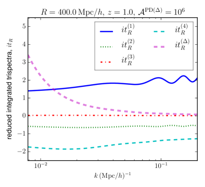
Figure 1: The various reduced integrated trispectra, $it_{R}^{(i)}$ (the expressions are given in Eq.(LABEL:eq:itRlocal) and Eq.(30)) for a large spherical sub-volume with radius $R=400\,{\rm Mpc}/h$ at $z=1.0$. We have taken $b_{1}=1.95,b_{2}=-0.18,b_{3}=-3.03$.

In Figure 1, we show the reduced integrated trispectra (or angle-averaged reduced position-dependent bispectrum) in the equilateral configuration from the leading-order perturbation theory, Eqs. (30), and from the local-type primordial trispectrum, Eq. (LABEL:eq:itRlocal).

In later Sections, we shall present forecasted cosmological constraints from the position-dependent power spectrum (integrated bispectrum) and from the position-dependent bispectrum (integrated trispectrum). In the squeezed-limit, the reduced integrated bispectrum induced by late-time gravitional evolution $ib_{\rm SPT}$ and the quadratic bias $ib_{b_{2}}$ are given by Chiang et al. (2014):

$$ib_{\rm SPT}(k) = \frac{1}{b_{1}}\left[\frac{47}{21}-\frac{1}{3}\frac{d\ln{P_{\delta}(k)}}{d\ln{k}}\right]$$ (31)

$$ib_{b_{2}}(k) = 2\frac{b_{2}}{b_{1}^{2}},$$ (32)

and, similarly, the integrated bispectrum from the local-type primordial non-Gaussianity ($f_{\rm NL}^{\rm local}$) is given by:

$$ib_{R}^{\left(f_{\rm NL}^{\rm local}\right)}(k) \approx \frac{4f_{\rm NL}^{\rm local}}{b_{1}\sigma_{R}^{2}}\int\frac{d^{3}\textbf{q}}{(2\pi)^{3}}\frac{W_{R}^{2}(q)}{V_{R}^{2}}\frac{P_{\delta}(q)}{\alpha(q)}.$$ (33)

So far, we have treated the primordial non-Gaussianity signal and late-time effects separately. Of course, primordial non-Gaussianity introduces a scale dependence in the galaxy bias, as convincingly demonstrated by Dalal et al. (2008). For models with long-short mode coupling of the local strength ($\beta=0$ case), the scale-dependent bias is given by a term that grows on large scales as $1/k^{2}$ and so the galaxy power spectrum can itself be used as a powerful constraint on $f_{\rm NL}^{\rm local}$ as well as $g_{\rm NL}^{\rm local}$ Baldauf et al. (2011); Smith et al. (2012); Tasinato et al. (2014). For SPHEREx, for example, forecasts find expected 1$\sigma$ uncertainty on estimating $f_{\rm NL}^{\rm local}$ to be $0.87$ from the power spectrum and $0.21$ from the bispectrum Doré et al. (2014). In this work, we focus on understanding the position-dependent bispectrum alone, so we shall leave the full treatment including the effect of long-short coupling to the non-Gaussian scale-dependent bias for future work.

V Fisher forecast method

We now present the Fisher information matrix formalism for the position-dependent power spectrum and bispectrum. Our method follows closely Chiang et al. (2015), but we restrict ourselves to the squeezed-limit of the reduced integrated bispectra and trispectra. The expression including full integration can be found in Chiang et al. (2015). Note also that we use the spherical top-hat window function instead of the cubic window function in Chiang et al. (2015). We calculate the linear matter power spectrum from the publically available CAMB Lewis et al. (2000) code by using the cosmological parameters from the Planck 2015 results (the TT+lowP+lensing column of Table 4 in Ade et al. (2016b)): $n_{s}=0.968,\sigma_{8}=0.815,\Omega_{m}=0.308,\Omega_{b}=0.048$.

Figure 2: The galaxy number density as a function of the redshift assumed in the Fisher matrix calculations. The function approximates the large galaxy count, low-accuracy redshift sample proposed for SPHEREx ($\tilde{\sigma}_{z}=0.1$, cumulative) in Figure 10 of Doré et al. (2014).

V.1 Reduced integrated bispectrum

The Fisher information matrix for measuring cosmological parameters $p_{\alpha}$ and $p_{\beta}$ from the reduced integrated bispectrum is given by

$$F_{ib_{R},\alpha\beta} = \sum_{z_{i}}N_{\rm sub}^{z_{i}}\sum_{R}\sum_{k\leq k_{\rm max}}$$ (34)

$$\frac{\partial ib_{R}(k,z_{i})}{\partial p_{\alpha}}\frac{\partial ib_{R}(k,z_{i})}{\partial p_{\beta}}\frac{1}{\Delta ib_{R}^{2}(k,z_{i})},$$

where we have considered the reduced integrated bispectrum up to wavenumber $k<k_{\rm max}$ for a fixed sub-volume size $R$. We then assume that the reduced integrated bispectrum with different sub-volume sizes are uncorrelated, so that we can add the information from different sub-volume sizes by simply summing different sub-volume radii $R$ (see, Section V.3 for the justification). Assuming that each sub-volume $V_{R}$ is identical, we multiplied the number of sub-volumes $N_{\rm sub}^{z_{i}}=V_{z_{i}}/\sum_{R}V_{R}$ with $V_{z_{i}}$ being the survey volume of the redshift bin centered around $z_{i}$. We approximate the uncertainties of measuring the reduced integrated bispectrum $ib_{R}(k)$ by its leading order, Gaussian covariance as

$$\Delta ib_{R}^{2}(k,z)=\frac{1}{N_{kR}}\frac{\left[\sigma_{R,z}^{2}+P_{\rm shot}/V_{R}\right]\left[P_{R,z}(k)+P_{\rm shot}\right]^{2}}{\sigma_{R,z}^{4}P_{R,z}^{2}(k)}$$ (35)

in which, $N_{kR}\approx 2\pi\left(k/k_{\rm min}\right)^{2}$ (with $k_{\rm min}\simeq\pi/R$) is the number of independent Fourier modes in a sub-volume Scoccimarro et al. (2004); Baldauf et al. (2011), and

$$P_{R,z}(k)=\frac{1}{V_{R}}\int\frac{d^{3}\textbf{q}}{(2\pi)^{3}}W_{R}^{2}(\textbf{q})P_{z}(|\textbf{k}-\textbf{q}|)$$ (36)

is the convolved power spectrum, and $P_{\rm shot}$ is the shot noise of the galaxy sample. Here, we assume that the galaxies are Poisson sample of the underlying density field so that $P_{\rm shot}=1/\bar{n}_{g}$ with the number density $\bar{n}_{g}$. As for the survey specifics, we adopt the survey volume and number density of the low-accuracy sample of the planned SPHEREx survey Doré et al. (2014). In Figure 2, we show the galaxy number density of the low-accuracy sample in Figure 10 of Doré et al. (2014).

V.2 Reduced integrated trispectrum

Similarly, the Fisher information matrix for the reduced integrated trispectrum is given by

$$F_{it_{R},\alpha\beta} = \sum_{z_{i}}N_{\rm sub}^{z_{i}}\sum_{R}\sum_{k\leq k_{\rm max}}$$ (37)

$$\frac{\partial it_{R}(k,z_{i})}{\partial p_{\alpha}}\frac{\partial it_{R}(k,z_{i})}{\partial p_{\beta}}\frac{1}{\Delta it_{R}^{2}(k,z_{i})},$$

with the covariance matrix (again, approximated by the leading order, diagonal part)

$$\Delta it_{R}^{2}(k,z)=\frac{V_{R}}{N_{k,\Delta}}\frac{\left[\sigma_{R,z}^{2}+P_{\rm shot}/V_{R}\right]\left[P_{R,z}(k)+P_{\rm shot}\right]^{3}}{\sigma_{R,z}^{4}P_{R,z}^{4}(k)}.$$ (38)

Here, $N_{k,\Delta}\approx(4/3)\pi^{2}\left(k/k_{\rm min}\right)^{3}$ is the number of independent equilateral-type triangular configurations (of size $k$) inside each sub-volume Baldauf et al. (2011).

V.3 Note on correlation matrix

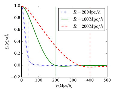
Figure 3: The smoothed two-point correlation function $\xi_{R}(r)$ as a function of the comoving distance $r$ (normalized by $\sigma_{R}^{2}$), for three smoothing scales $R=200,100,20\,{\rm Mpc}/h$. The vertical lines are $r=2R$ lines, and are plotted to show that the correlation is small for sub-volumes separated by $r>2R$.

When calculating the Fisher information matrix, we have assumed that there is no cross-correlation among locally calculated power spectra and bispectra from different sub-volumes. To see that this is a reasonable approximation, note that the dominant contribution for the matrix element $\Big{\langle}it_{R}(k,\textbf{x})it_{R}(k,\textbf{x}^{\prime})\Big{\rangle}$ separated by $|\textbf{x}^{\prime}-\textbf{x}|=r$ is given by

$$\Big{\langle}it_{R}(k,\textbf{x})it_{R}(k,\textbf{x}^{\prime})\Big{\rangle}\approx\frac{V_{R}}{N_{k,\Delta}}\frac{\xi_{R}(r)}{\sigma_{R}^{2}P_{R}(k)}$$ (39)

where,

$$\xi_{R}(r)=\frac{1}{V_{R}^{2}}\int\frac{q^{2}dq}{2\pi^{2}}W_{R}^{2}(q)P(q)j_{0}(qr),$$ (40)

is the two-point correlation function of the density field smoothed over the size of the sub-volume.

We plot the smoothed correlation function $\xi_{R}(r)/\sigma_{R}^{2}$ in Figure 3. In the zero shot noise limit, the off-diagonal element of the covariance matrix can be well approximated by $\xi_{R}(r)/\sigma_{R}^{2}$ (for both the integrated bispectrum and integrated trispectrum). In the presence of shot noise, we expect the normalized matrix element (non-diagonal) to be smaller. For each $R$, we see that the correlation is very weak when $r>2R$, which is the distance between the centers of adjacent two sub-volumes. In addition, there must be some correlation from non-Gaussian coupling to very long wavelength modes common to neighboring sub-volumes, but the scale dependence of the integrands in Eq. (5), Eq. (III.2) indicates that this should be small.

We have also assumed the reduced trispectra at different wavenumbers are uncorrelated. That is

$$\Big{\langle}it_{R}(k_{1})it_{R}(k_{2})\Big{\rangle}\approx\delta_{D}(k_{1}-k_{2})\Delta it_{R}^{2}(k)$$

(and similarly for the integrated bispectrum). This approximation breaks down at smaller scales and lower redshifts when non-linearities are strong Chiang (2015) (see in particular Figure B.1. and the discussion around it in the Ref. Chiang (2015)). It is also worthwhile to note other important results from Chiang (2015): (i) that the cross correlation between integrated bispectrum with different $k$ values with different sub-volume sizes gets weaker, because different long-wavelength modes are involved, (ii) that having different sized sub-volumes and different redshifts is useful in breaking the degeneracy between the primordial and late-time contributions to the integrated bispectrum. This is because, the primordial integrated bispectrum signal depends on the sub-volume size (through $\sigma_{R}^{2}$) and is also inversely proportional to the growth factor $D(z)$ whereas the late time contributions are nearly independent of these. Similarly, we see that the reduced integrated trispectrum signal (primordial) has different $z$ and $R$ dependence compared to the late time contribution.

Note that at a given single redshift, $ib_{R}^{(f_{\rm NL}^{\rm local})}$ (in the squeezed limit) and $ib_{b_{2}}$ are both constant and therefore degenerate. It is, therefore, necessary to use more than one sub-volume sizes to break this degeneracy for a single redshift bin. On the other hand, for the integrated trispectrum, such a strong degeneracy is absent (see Figure 1). The results of our Fisher matrix analysis considering multiple redshift bins in the range $0.1<z<3.0$, and using the number density expected for the SPHEREx survey is presented next.

VI Fisher forecast results

We now present results from the Fisher matrix analysis. We will focus on the projected constraints on the non-Gaussianity amplitudes $f_{\rm NL}^{\rm local}$ and $\mathcal{A}^{{\rm PD}(\triangle)}$. The fiducial values we use for this analysis are: $f_{\rm NL}^{\rm local}=0\,{\rm and}\,\mathcal{A}^{{\rm PD}(\triangle)}=0$. For the SPHEREx survey, we use a constant fiducial linear bias parameter $b_{1}=1.95$ and compute the non-linear bias parameters $b_{2}$ and $b_{3}$ using the fitting functions in Table 3 of Desjacques et al. (2016).

VI.1 $f_{\rm NL}^{\rm local}$ constraint from integrated bispectrum

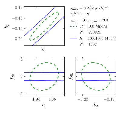
Figure 4: Fisher forecast ellipses for two of $(f_{\rm NL}^{\rm local},b_{1},b_{2})$ marginalized over the other, assuming SPHEREx survey volume and other parameters given above in the figure. See Figure 2 for the assumed galaxy number density as a function of the redshift. The two different ellipses in each plot represent different choices for sub-volumes: (i) dashed green – only one type of sub-volume with radius $R=100\;{\rm Mpc}/h$; this means that the total number of sub-volumes when dividing the whole survey is large ($N=260924$), (ii) solid blue – two sizes of sub-volumes with $R=100,1000\;{\rm Mpc}/h$ in equal numbers (except for when the volume of a redshift bin is smaller than the volume of the larger sub-volume). The Fisher constraint for these two cases are: $\sigma(f_{\rm NL})=4.0,1.2$; $\sigma(b_{1})=0.02,0.16$ and $\sigma(b_{2})=0.03,0.22$.

In Figure 4, we show the projected $1-\sigma$ (68% confidence level) error ellipse for $f_{\rm NL}$ and the bias parameters using the integrated bispectrum. We can see that constraints of order $\sigma(f_{\rm NL})\approx 1$ is possible with SPHEREx survey by using the integrated bispectrum method. This result is the same order of magnitude with the projection obtained in Doré et al. (2014) using the full bispectrum. However, we note that we have not included the scale-dependent bias from local primordial non-Gaussianity (which dominates the constraint in Doré et al. (2014)) nor optimized the sub-volume choices. Therefore, it must be possible to further improve the constraint.

Survey	$R\;({\rm Mpc}/h)$	$N_{\rm sub-volumes}$	$\sigma(f_{\rm NL})$
SPHEREx	100, 1000	1302	1.20
SPHEREx	$[1,2,3,4,5]\times 100$	5775	1.71
eBOSS LRGs	200, 500	$408$	20.5
eBOSS quasars	200, 500	$1750$	54.5

Table 1: Fisher forecast results for $f_{\rm NL}$. In the first row, we have considered two sub-volume sizes: one large $R=1000{\;{\rm Mpc}/h}$ ($N=255$) and one small: $R=100{\;{\rm Mpc}/h}$ ($N=1047$). In the second row, we have used five different sub-volume sizes: $R=100,200,300,400,500{\;{\rm Mpc}/h}$; there are $1155$ of each of these sub-volumes.

In addition, in Table 1, we also list Fisher constraint on $f_{\rm NL}$ by considering the luminous red galaxies (LRGs) and the quasars from the extended Baryon Oscillation Spectroscopic Survey (eBOSS). We take the survey parameters, the expected number densities, and the bias parameters from Zhao et al. (2016) (See Table 2 in the reference).

VI.2 $\mathcal{A}^{{\rm PD}(\triangle)}$ constraint from integrated trispectrum

Figure 5: Fisher forecast ellipses for two of $(\mathcal{A}^{{\rm PD}(\triangle)},b_{1},b_{2})$ marginalized over the other and $b_{3}$ (which is not shown), assuming SPHEREx survey volume. The different colored ellipses represent different sets of sub-volume types: (i) dashed green – only one type of sub-volume with radius $R=200\;{\rm Mpc}/h$, (ii) solid blue – two sizes of sub-volumes with $R=200,500\;{\rm Mpc}/h$ in equal numbers. The Fisher constraints for these two cases are: $\sigma(\mathcal{A}^{{\rm PD}(\triangle)})=1.57\times 10^{6}$, $2.49\times 10^{6}$; $\sigma(b_{1})=2.9,10.2$; $\sigma(b_{2})=3.0,10.6$. Note that while the two figures in the bottom panel look very similar, they have slightly different $1-\sigma$ errors for $b_{1}$ and $b_{2}$.

Survey	$R\;({\rm Mpc}/h)$	$N_{\rm sub-volumes}$	$\sigma(\mathcal{A}^{{\rm PD}(\triangle)})$	$\sigma(g_{\rm NL}^{\rm local})$
SPHEREx	$[1,2,3,4,5]\times 100$	5775	$1.85\times 10^{6}$	$3.08\times 10^{5}$
SPHEREx	200, 500	3912	$2.49\times 10^{6}$	$4.15\times 10^{5}$
SPHEREx	100, 1000	1302	$4.04\times 10^{6}$	$6.73\times 10^{5}$
eBOSS LRGs	200, 500	$408$	$1.80\times 10^{7}$	$3.00\times 10^{6}$
eBOSS quasars	200, 500	$1750$	$6.43\times 10^{7}$	$1.07\times 10^{7}$

Table 2: Fisher forecast results for $\mathcal{A}^{{\rm PD}(\triangle)}$. In the last column, we have translated the constraint on $\mathcal{A}^{{\rm PD}(\triangle)}$ to the constraint on the local-type primordial trispectrum amplitude $g_{\rm NL}^{\rm local}$ using $g_{\rm NL}^{\rm local}={\mathcal{A}^{{\rm PD}(\triangle)}}/{6}$.

In Figure 5, we show the projected $1-\sigma$ (68% confidence level) error ellipse for $\mathcal{A}^{{\rm PD}(\triangle)}$ and the bias parameters using the integrated trispectrum. With the same survey parameters that was used for $f_{\rm NL}$, we obtain $\sigma(\mathcal{A}^{{\rm PD}(\triangle)})\approx 10^{6}$. See Table 2 for a list of constraints on the non-Gaussianity parameter $\mathcal{A}^{{\rm PD}(\triangle)}$ and the corresponding constraint on $g_{\rm NL}^{\rm local}$ for other choices of subvolume sizes. By using only the equilateral configuration of the bispectrum, we can obtain $\sigma(g_{\rm NL}^{\rm local})\approx 3\times 10^{5}$. By adding the position dependence of the other triangular configurations, we should expect improvements in the $g_{\rm NL}^{\rm local}$ constraints. Note that this is different than the case of $f_{\rm NL}^{\rm local}$ using integrated bispectrum in which we use all the power spectra in the “position-dependent power spectrum”. In the equilateral configuration, the total number of triangles used is roughly given by

$$N_{{\rm equil},\Delta}\approx 2\pi^{2}\left(\frac{k_{\rm max}}{k_{\rm min}}\right)^{4}.$$

If we use all the triangles possible, however, then the rough count of the number of triangles becomes

$$N_{{\rm all},\Delta}\approx\pi^{2}\left(\frac{k_{\rm max}}{k_{\rm min}}\right)^{6}.$$

Therefore, if we assume that the ratio of the primordial contribution to the late-time contributions to the integrated trispectrum do not change drastically when considering non-equilateral configurations, we can estimate the approximate improvement expected in the $g_{\rm NL}^{\rm local}$ constraint when including all triangular configurations by taking the square root of the ratio $N_{\rm all,\Delta}/N_{\rm equil,\Delta}$. That is roughly one expects improvement of the order $\mathcal{O}\left(k_{\rm max}/k_{\rm min}\right)$; so, it is reasonable to expect an improvement to $\sigma(g_{\rm NL}^{\rm local})$ by a factor of 10 than what is obtained in our Fisher forecasts (with only the equilateral configuration). In that case, $\sigma(g_{\rm NL}^{\rm local})\approx 10^{4}$ may be possible with the SPHEREx survey using the position-dependent bispectrum method, which is nearly a factor of 10 better than the current best constraint from Planck satellite.

VII Conclusions

We have developed the “position-dependent bispectrum,” a higher-order extension of the position-dependent power spectrum in Ref. Chiang et al. (2014). We have shown that, when applied to galaxy surveys, this new observable can open up a new and efficient avenue of measuring the four-point correlation functions in the squeezed limit; through the method, the galaxy surveys can be an even more powerful probe of primordial non-Gaussianities. We have shown that the projected uncertainty of measuring $g_{\rm NL}^{\rm local}$ from a SPHEREx-like galaxy survey is already comparable to that of Planck result ($\sigma(g_{\rm NL}^{\rm local})\approx 10^{5}$). But, this result is obtained by using only a small subset (equilateral configuration of the local bispectra) of all the available triangles, and we expect an order-of-magnitude better constraint by using all triangular configurations. For the constraint on $f_{\rm NL}^{\rm local}$, we find that the position-dependent power spectrum with SPHEREx survey can provide $\sigma(f_{\rm NL}^{\rm local})\approx 1$; this value is consistent with the previous studies if one restricts to the squeezed-limit of the galaxy bispectrum.

One goal of constraining the position dependence of the statistics like the power spectrum and bispectrum is to bound the non-Gaussian cosmic variance that may affect the translation between properties of the observed fluctuations and the particle physics of the primordial era. This cosmic variance arises from the coupling of modes inside our Hubble volume (that we observe from, for example, galaxy surveys) to the unobservable modes outside. For scenarios with mode coupling of the local strength ($\beta=0$ for the coupling of the bispectrum to long wavelength modes), the cosmic variance uncertainty can be significant even for very low levels of observed non-Gaussianity. For example, consider a universe with a trispectrum of the sort given in Eq. (17), that induces a bispectrum of the equilateral type in biased sub-volumes. As plotted in Baytaş et al. (2015), if our Hubble volume has values of $f_{\rm NL}^{\rm equil}=10$, $g_{\rm NL}^{\rm equil}=5\times 10^{3}$, the value of $f_{\rm NL}^{\rm equil}$ in an inflationary volume with 100 extra e-folds can be between 0 and 20 at $1-\sigma$ ($68\%$ confidence level). From Table 2, this value of $g_{\rm NL}^{\rm equil}$ ($=\mathcal{A}^{{\rm PD}(\triangle)}/2)$ is more than two orders of magnitude below our rough estimate of what can be ruled out by a SPHEREx like survey, and so is unlikely to be reached even by including more configurations of the bispectrum. If models that can generate a trispectrum like that in Eq. (17) are physically reasonable (which is certainly possible, although we have not yet investigated in detail), it will be hard to conclusively tie a detection of $f_{\rm NL}^{\rm equil}$ to single-clock inflation, unless we have other ways of quantifying the non-Gaussian cosmic variance.

We have made several approximations here in order to convey the basic utility of the position-dependent bispectrum, and there are many ways in which our analysis can be improved. In particular, we have not included complimentary, and potentially very significant, information from the scale-dependent bias, nor the information from higher order position-dependent power spectrum correlations (e.g, $\langle P(\textbf{k})_{\textbf{x}_{R}}\bar{\delta}_{\textbf{x}_{R}}^{2}\rangle$), which would further distinguish trispectra configurations. To obtain the best constraint from a given galaxy survey (e.g. SPHEREx that we adopted here), we should also extend the position-dependent bispectrum to include more general triangular configurations and optimize the selection sub-volume sizes and numbers. We will address these issues in future work.

Appendix A Trispectrum expressions

Here we list the expression for galaxy trispectrum induced by late time non-linear gravitational evolution and non-linear bias, taken from Sefusatti and Scoccimarro (2005). We assume that the primordial fluctuations follow Gaussian statistics. See Eq. (29) for the full expression including the galaxy bias parameters.

$$T^{(1)} = T_{a}+T_{b}$$ (41)

$$T^{(2)} = 4P_{1}\left[F_{2}^{(s)}(\textbf{k}_{2},\textbf{k}_{3})P_{2}P_{3}+F_{2}^{(s)}(\textbf{k}_{2},-\textbf{k}_{23})P_{2}P_{23}+F_{2}^{(s)}(\textbf{k}_{3},-\textbf{k}_{23})P_{3}P_{23}\right]+4P_{2}\left[F_{2}^{(s)}(\textbf{k}_{1},\textbf{k}_{3})P_{1}P_{3}\right.$$

$$+\left.F_{2}^{(s)}(\textbf{k}_{1},-\textbf{k}_{13})P_{1}P_{13}+F_{2}^{(s)}(\textbf{k}_{3},-\textbf{k}_{13})P_{3}P_{13}\right]+4P_{3}\left[F_{2}^{(s)}(\textbf{k}_{1},\textbf{k}_{2})P_{1}P_{2}+F_{2}^{(s)}(\textbf{k}_{1},-\textbf{k}_{12})P_{1}P_{12}\right.$$

$$+\left.F_{2}^{(s)}(\textbf{k}_{2},-\textbf{k}_{12})P_{2}P_{12}\right]+(3~{}{\rm cyc.})$$

$$T^{(3)} = 4P_{1}P_{2}(P_{13}+P_{14})+(5~{}{\rm perm.})$$

$$T^{(4)} = 6P_{1}P_{2}P_{3}+(3~{}{\rm cyc.})$$ (42)

$${\rm where}$$

$$T_{a} = 4P_{1}P_{2}[P_{13}F_{2}^{(s)}(\textbf{k}_{1},-\textbf{k}_{13})F_{2}^{(s)}(\textbf{k}_{2},\textbf{k}_{13})+P_{14}F_{2}^{(s)}(\textbf{k}_{1},-\textbf{k}_{14})F_{2}^{(s)}(\textbf{k}_{2},\textbf{k}_{14})]+(5~{}{\rm perm.})$$

$$T_{b} = 6F_{3}^{(s)}(\textbf{k}_{1},\textbf{k}_{2},\textbf{k}_{3})P_{1}P_{2}P_{3}+(3~{}{\rm cyc.})$$

where the symmetrized perturbation theory kernels are given by (See, Bernardeau et al. (2002) for a review)

$$F_{2}^{(s)}(\textbf{k}_{1},\textbf{k}_{2}) = \frac{5}{7}+\frac{1}{2}\frac{\textbf{k}_{1}\cdot\textbf{k}_{2}}{k_{1}k_{2}}\left(\frac{k_{1}}{k_{2}}+\frac{k_{2}}{k_{1}}\right)+\frac{2}{7}\left(\hat{k}_{1}\cdot\hat{k}_{2}\right)^{2}$$ (44)

$$G_{2}^{(s)}(\textbf{k}_{1},\textbf{k}_{2}) = \frac{3}{7}+\frac{1}{2}\frac{\textbf{k}_{1}\cdot\textbf{k}_{2}}{k_{1}k_{2}}\left(\frac{k_{1}}{k_{2}}+\frac{k_{2}}{k_{1}}\right)+\frac{4}{7}\left(\hat{k}_{1}\cdot\hat{k}_{2}\right)^{2}$$ (45)

$$F_{3}^{(s)}(\textbf{k}_{1},\textbf{k}_{2},\textbf{k}_{3}) = \frac{2k_{123}^{2}}{54}\left[\frac{\textbf{k}_{1}\cdot\textbf{k}_{23}}{k_{1}^{2}k_{23}^{2}}G_{2}^{(s)}(\textbf{k}_{2},\textbf{k}_{3})+(2~{}{\rm cyc.})\right]+\frac{7}{54}\left[\frac{\textbf{k}_{123}\cdot\textbf{k}_{23}}{k_{23}^{2}}G_{2}^{(s)}(\textbf{k}_{2},\textbf{k}_{3})+(2~{}{\rm cyc.})\right]$$ (46)

$$+\frac{7}{54}\left[\frac{\textbf{k}_{123}\cdot\textbf{k}_{1}}{k_{1}^{2}}F_{2}^{(s)}(\textbf{k}_{2},\textbf{k}_{3})+(2~{}{\rm cyc.})\right].$$

By directly taking the appropriate equilateral and soft limit $|\textbf{k}_{4}|=q\rightarrow 0$, and after angular averaging, we can get the integrated trispectrum $iT_{R}^{(1)}(k)$. For example, for the two terms in $T^{(1)}$, we obtain

$$\Big{\langle}T_{a}(k)\Big{\rangle}_{\rm angle-avg} = P_{\delta}^{2}(k)P_{\delta}(q)\left[\frac{585}{147}-\frac{20}{21}\frac{\partial\ln{P_{\delta}(k)}}{\partial\ln{k}}\right]$$

$$\Big{\langle}T_{b}(k)\Big{\rangle}_{\rm angle-avg} = P_{\delta}^{2}(k)P_{\delta}(q)\left[\frac{27}{14}-\frac{4}{21}\frac{\partial\ln{P_{\delta}(k)}}{\partial\ln{k}}\right]$$

$$\implies iT^{(1)}(k) = P_{\delta}^{2}(k)P_{\delta}(q)\left[\frac{579}{98}-\frac{8}{7}\frac{\partial\ln{P_{\delta}(k)}}{\partial\ln{k}}\right]$$