Hybrid CPU-GPU Framework for Network Motifs

Abstract

Massively parallel architectures such as the GPU are becoming increasingly important due to the recent proliferation of data. In this paper, we propose a key class of hybrid parallel graphlet algorithms that leverages multiple CPUs and GPUs simultaneously for computing k-vertex induced subgraph statistics (called graphlets). In addition to the hybrid multi-core CPU-GPU framework, we also investigate single GPU methods (using multiple cores) and multi-GPU methods that leverage all available GPUs simultaneously for computing induced subgraph statistics. Both methods leverage GPU devices only, whereas the hybrid multi-core CPU-GPU framework leverages all available multi-core CPUs and multiple GPUs for computing graphlets in large networks. Compared to recent approaches, our methods are orders of magnitude faster, while also more cost effective enjoying superior performance per capita and per watt. In particular, the methods are up to 300 times faster than a recent state-of-the-art method. To the best of our knowledge, this is the first work to leverage multiple CPUs and GPUs simultaneously for computing induced subgraph statistics.

[parallel]parallelforparallelend [1][]parallel for #1 end parallel EndFor EndIf EndProcedure EndParallel [parallel]parforendpar[1][]parallel for #1 doend parallel

1 Introduction

Graphlets are small $k$-vertex induced subgraphs and are important for many predictive and descriptive modeling tasks (prvzulj2004modeling; milenkoviae2008uncovering; hayes2013graphlet) in a variety of disciplines including bioinformatics (vishwanathan2010graph; shervashidze2009efficient), cheminformatics (rupp2010graph), and image processing and computer vision (zhang-image-categorization-via-graphlets; zhang2013probabilistic). Given a network $G$, our approach counts the frequency of each $k$-vertex induced subgraph patterns (See Table 1). These counts represent powerful features that succinctly characterize the fundamental network structure (shervashidze2009efficient). Indeed, it has been shown that such features accuratly capture the local network structure in a variety of domains (Holland_Lein; faust2010puzzle; frank1988triad). As opposed to global graph parameters such as diameter for which two or more networks may have global graph parameters that are nearly identical, yet their local structural properties may be significantly different.

Despite the practical importance of graphlets, existing algorithms are slow and are limited to small networks (e.g., even modest graphs can take days to finish), require vast amounts of memory/space-inefficient, are inherently sequential (inefficient and difficult to parallelize), and have many other issues. Overcoming the slow performance and scalability limitations of existing methods is perhaps the most important and challenging problem remaining. This work proposes a fast hybrid parallel algorithm for computing both connected and disconnected subgraph statistics (of size $k$) including macro-level statistics for the global graph $G$ as well as micro-level statistics for individual graph elements such as edges. Furthermore, a number of important machine learning tasks are likely to benefit from the proposed methods, including graph anomaly detection (noble2003graph; akoglu2014graph), entity resolution (bhattacharya2006entity), as well as features for improving community detection (schaeffer2007graph), role discovery (rossi2014roles), and relational classification (getoor2007introduction).

The recent rise of Big Data has brought many challenges and opportunities (boyd2012critical; ahmed2014graph; ahmed12socialnets). Recent heterogeneous high performance computing (HPC) architectures offer viable platforms for addressing the computational challenges of mining and learning with big graph data. General-purpose graphics processing units (GPGPUs) (brodtkorb2013graphics) are becoming increasingly important with applications in scientific computing, machine learning, and many others (gharaibeh2013energy). Heterogeneous (hybrid) computing architectures consisting of multi-core CPUs and multiple GPUs are an attractive alternative to traditional homogeneous HPC clusters (HPCC). Despite the impressive theoretical performance achievable by such hybrid architectures, leveraging this computing power remains an extremely challenging problem.

Graphics processing units (GPUs) offer cost-effective high-performance solutions for computation-intensive data mining applications. As an example, the Nvidia Titan Black GPU has 2880 cores capable of performing over 5 trillion floating-point operations per second (TFLOPS). For comparison a Xeon E5-2699v3 processor can perform about 0.75 TFLOPS, but can cost 4x as much. Besides TFLOPS, GPUs also enjoy a significant advantage over CPUs in terms of memory bandwidth, which is more important for data-intensive algorithms such as graphlet decomposition. For Titan Black, its maximum memory bandwidth is 336 GB/sec; whereas E5-2699v3’s is only 68 GB/sec. Higher memory bandwidth means more graph edges can be traversed on the GPU than the CPU in the same amount of time, which is one of the main reasons why our approach can outperform the state-of-the-art.

However, unlike the single GPU-based approach proposed in (milinkovic14contribution), we adopt a hybrid parallelization strategy that exploits the complementary features of multiple GPUs and CPUs to achieve significantly better performance. We begin with the key observation that the amount of work required to compute graphlets for each edge in $G$ obeys a power-law (See Figure 1). Strikingly, a handful of edges require a lot of work to determine the local graphlet counts (due to the density and structure of the local edge neighborhood), whereas the vast majority of other edges require only a small amount of work. Such heterogeneity can cause significant load balancing issues, especially for GPUs that are designed to solve problems with uniform workloads (e.g., dense matrix-matrix multiplications). This motivates our hybrid approach that dynamically divides up the work between GPU and CPU, to reduce inter-processor communication, synchronization and data transfer overheads.

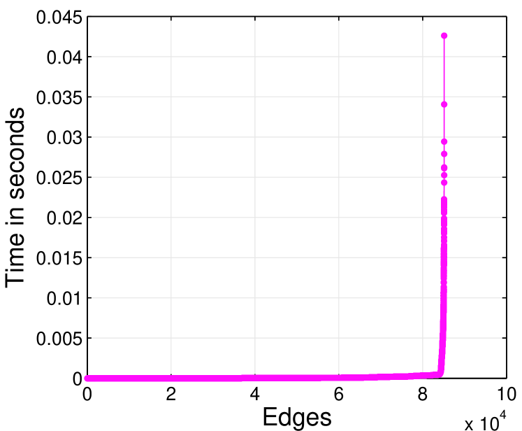
Figure 1: The distribution of graphlet computation times for the edge neighborhoods obey a power-law. The time taken to count $k=\{2,3,4\}$ graphlets for each edge is shown above and clearly obeys a power-law distribution (${\mathsf{tech}\text{--}{\mathbf{\tt internet\text{-}as}}}$).

This work demonstrates that parallel graphlet methods designed for heterogeneous computing architectures consisting of many multi-core CPUs and multiple GPUs can significantly improve performance over GPU-only and CPU-only approaches. In particular, our hybrid CPU-GPU framework is designed to leverage the advantages and key features offered by each type of processing unit (multi-core CPUs and GPUs). As such, our approach leverages the fact that graphlets can be computed via $M$ independent edge-centric neighborhood computations. Therefore, the method dynamically distributes the edge-centric graphlet computations to either a CPU or a GPU. In particular, the edge-centric graphlet computations that are fundamentally unbalanced and highly-skewed are given to the CPUs whereas the GPUs work on the more well-balanced and regular edge neighborhoods (See Figure LABEL:fig:graphlet-cpu-gpu-runtime). These approaches capitalize on the fact that GPUs are generally best for computations that are well-balanced and regular, whereas CPUs are designed for a wide variety of applications and thus more flexible (lee2010debunking; malony2011parallel). Our approach also leverages dynamic load balancing and work stealing strategies to ensure all GPU and CPU workers (cores) remain fully utilized.

2 Related Work

Recently, Milinković et al. (milinkovic14contribution) proposed a GPU algorithm for counting graphlets based on a recent sequential graphlet algorithm called orca (orca). However, this paper is fundamentally different. First and foremost, that approach is not hybrid and is only able to use a single GPU for computing graphlets. In addition, that work focuses on computing connected graphlets only, whereas we compute both connected and disconnected induced subgraphs. Moreover, that approach computes graphlets for each vertex in parallel (vertex-centric), whereas our methods are naturally edge-centric and search edge neighborhoods in parallel. Furthermore, that work does not provide any comparison to understand the utility and speedup (if any) offered by their approach.

In this work, we propose a heterogeneous graphlet framework for hybrid multi-GPU and CPU systems that leverages all available GPUs and CPUs for efficient graphlet counting. Our single-GPU, multi-GPU, and hybrid CPU-GPU algorithms are largely inspired by the recent state-of-the-art parallel (CPU-based) exact graphlet decomposition algorithm called pgd (pgd-kais; nkahmed:icdm15), which is known to be significantly faster and more efficient than other methods including rage (rage), fanmod (fanmod), and orca (orca). Moreover, pgd has been parallelized for multi-core CPUs and is publicly available. Our approach is evaluated against pgd and a recent orca-GPU approach in Section LABEL:sec:exp.

Table 1: Summary of the graphlet notation

Graphlets are grouped by number of vertices ($k$-graphlets) and categorized into connected and disconnected graphlets. Connected graphlets of each size are then ordered by density. The complement of each connected graphlet is shown on the right and represent the disconnected graphlets. Note $4$-path is a self-complementary${}^{\star}$. Graphlets of size $k$=2 are included for completeness.
	$\mathbf{k}$		Connected			Disconnected
graphlets	$\mathbf{2}$			${H}_{1}$	edge		${H}_{2}$	2-node-indep.
	$\mathbf{3}$			${H}_{3}$	triangle		${H}_{6}$	3-node-indep.
				${H}_{4}$	2-star		${H}_{5}$	3-node-1-edge
	$\mathbf{4}$			${H}_{7}$	4-clique		${H}_{17}$	4-node-indep.
				${H}_{8}$	chordal-cycle		${H}_{16}$	4-node-1-edge
				${H}_{9}$	tailed-triangle		${H}_{15}$	4-node-2-star
				${H}_{10}$	4-cycle		${H}_{14}$	4-node-2-edge
				${H}_{11}$	3-star		${H}_{13}$	4-node-1-triangle
				${H}_{12}$	4-path${}^{{}_{\star}}$

3 Graphlet Decomposition

Graphlets are at the heart and foundation of many network analysis tasks (e.g., relational classification, network alignment) (prvzulj2004modeling; milenkoviae2008uncovering; hayes2013graphlet). Given the practical importance of graphlets, this paper proposes a hybrid CPU-GPU algorithm for computing the number of embeddings for both connected and disconnected k-vertex induced subgraphs (See Table 1).

3.1 Preliminaries

Let $G=(V,E)$ be an undirected graph where $V$ is the set of vertices and $E$ is its edge set. The number of vertices is $n=|V|$ and number of edges is $m=|E|$. We assume all vertex and edge sets are ordered, i.e., $V=\{v_{1},v_{2},...,v_{i},...,v_{N}\}$ such that $v_{i-1}$ appears before $v_{i}$ and so forth. Similarly, the ordered edges are denoted $E=\{e_{1},e_{2},...,e_{i},...,e_{M}\}$. Given a vertex $v\in V$, let $\Gamma(v)=\{w|(v,w)\in E\}$ be the set of vertices adjacent to $v$ in $G$. The degree $d_{v}$ of $v\in V$ is the size of the neighborhood $|\Gamma(v)|$ of $v$. We also define $\Delta$ to be the largest degree in $G$.

Definition 1 (Graphlet)

A graphlet ${H}_{i}=(V_{k},E_{k})$ is a subgraph consisting of a subset $V_{k}\subset V$ of $k$ vertices from $G=(V,E)$ together with all edges whose endpoints are both in this subset $E_{k}=\{\forall e\in E\,|\,e=(u,v)\wedge u,v\in V_{k}\}$.

Let ${\mathcal{H}}^{(k)}$ denote the set of $k$-vertex induced subgraphs and ${\mathcal{H}}={\mathcal{H}}^{(2)}\cup\cdots\cup{\mathcal{H}}^{(k)}$. A $k$-graphlet is simply an induced subgraph with k-vertices.

3.2 Problem Formulation

It is important to distinguish between the two fundamental classes of graphlets, namely, connected and disconnected graphlets (see Table 1). A graphlet is connected if there is a path from any node to any other node in the graphlet (see Definition 2). Table 1 provides a summary of the connected and disconnected k-graphlets of size $k=\{2,3,4\}$.

Definition 2 (Connected graphlet)

A $k$-graphlet ${H}_{i}=(V_{k},E_{k})$ is connected if there exists a path from any vertex to any other vertex in the graphlet ${H}_{i}$, $\forall u,v\in V_{k},$ $\exists P_{u-v}:u,\ldots,w,\ldots,v$, such that $d(u,v)\geq 0\wedge d(u,v)\neq\infty$. By definition, a connected graphlet ${H}_{i}$ has only one connected component (i.e., $|C|=1$).

Definition 3 (Disconnected graphlet)

A $k$-graphlet ${H}_{i}=(V_{k},E_{k})$ is disconnected if there is not a path from any vertex $v\in{H}_{i}$ to any other vertex $w\in{H}_{i}$.

Unlike most existing work that is only able to compute connected graphlets of a certain size (such as $k=4$), the goal of this work is to compute the frequency of both connected and disconnected graphlets of size $k\in\{2,3,4\}$. More formally,

Problem 1 (Global graphlet counting)

Given the graph $G$, find the number of embeddings (appearances) of each graphlet ${H}_{i}\in{\mathcal{H}}$ in the input graph $G$. We refer to this problem as the global graphlet counting problem. A graphlet ${H}_{i}\in{\mathcal{H}}$ is embedded in $G$, iff there is an injective mapping $\sigma:V_{{H}_{i}}\rightarrow V$, with $e=(u,v)\in E_{{H}_{i}}$ if and only if $e^{\prime}=(\sigma(u),\sigma(v))\in E$.

4 Hybrid CPU-GPU Framework

This work proposes parallel graphlet decomposition methods that are designed to leverage (i) parallelism (multiple cores on a CPU or GPU) as well as (ii) heterogeneity that leverages simultaneous use of a CPU and GPU (as well as multiple CPUs and GPUs). To the best of our knowledge, this is the first work to use multiple GPUs (and of course multiple GPUs and CPUs) for computing induced subgraph statistics.

• Single GPU Methods (using multiple cores)

• Multi-GPU Methods.

• Hybrid Multi-core CPU-GPU Methods.

Methods from all three classes are shown to be effective on a large collection of graphs from a variety of domains (e.g., biological, social, and information networks (nr-aaai15)). In particular, methods from these classes have three important benefits. First, the performance is orders of magnitude faster than the state-of-the-art. Second, the GPU methods are cost effective enjoying superior performance per capita. Third, the performance per watt is significantly better than existing traditional CPU methods.

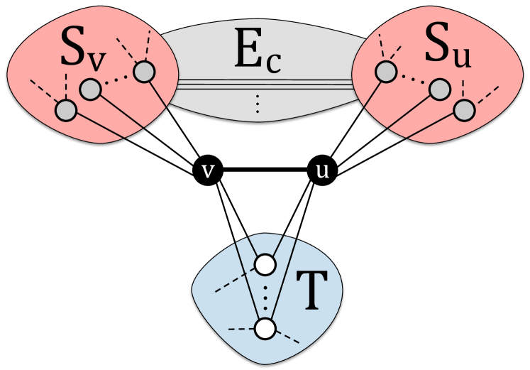
Figure 2: Let ${T}$ be the set of nodes completing a triangle with the edge $(v,u)\in E$, and let ${S}_{v}$ and ${S}_{u}$ be the set of nodes that form a 2-star with $v$ and $u$, respectively. Note that ${S}_{u}\cap{S}_{v}=\emptyset$ by construction and $|{S}_{u}\cup{S}_{v}|=|{S}_{u}|+|{S}_{v}|$. Further, let $E_{c}$ be the set of edges that complete a cycle (of size 4) w.r.t. the edge $(v,u)$ where for each edge $(p,q)\in E_{c}$ such that $p\in{S}_{v}$ and $q\in{S}_{u}$ and both $(p\cap{S}_{u})\cup(q\cap{S}_{v})=\emptyset$, that is, $p$ is not adjacent to $u$ ($p\not\in\Gamma(u)$) and $q$ is not adjacent to $v$ ($q\not\in\Gamma(v)$).

4.1 Parallel Graphlet Computations

Our algorithm searches over the set of edges $E$ of the input graph $G=(V,E)$. Given an edge $e=(u,v)\in E$, let $\Gamma(e)$ denote the edge neighborhood of $e$ defined as:

$$\Gamma(e)=\Gamma(u,v)=\{\Gamma(u)\cup\Gamma(v)\setminus\{u,v\}\},$$ (1)

where $\Gamma(u)\textrm{ and }\Gamma(v)$ are the neighbors of $u\textrm{ and }v$, respectively. For convenience, let $\boldsymbol{\Gamma}_{e}=G(\{\Gamma(v)-u\}\cup\{\Gamma(u)-v\})$ be the (explicit) edge-induced neighborhood subgraph. Given an edge $e=(u,v)\in E$, we explore the subgraph surrounding $e$ (called the egonet of $e$), i.e., the subgraph induced by both its endpoints and the vertices in its neighborhood. Our approach uses a specialized graph encoding based on the edge-CSC representation (rossi2014tcore).

The parallel scheme leverages the fact that the induced subgraph (graphlet) problem can be solved independently for each edge-centric neighborhood $\Gamma(e_{i})\in\{\Gamma(e_{1}),\ldots,\Gamma(e_{M})\}$ in $G$, and therefore may be computed simultaneously in parallel. A processing unit denoted by $\omega$ refers to a single CPU/GPU worker (core). In the context of message-passing and distributed memory parallel computing, a node refers to another machine on the network with its own set of multi-core CPUs, GPUs, and memory. Other important properties include the search order $\Pi$ in which edges are solved in parallel, the batch size $b$ (number of jobs/tasks assigned to a worker by a dynamic scheduling routine), and the dynamic assignment of jobs (for load balancing).

While there are only a few such parallel graphlet algorithms, with the exception of pgd all of these methods are based on searching over the vertices (as opposed to the edges). However, as we shall see, the parallel performance of these approaches are guaranteed to suffer more from load balancing issues, communication costs, and other issues such as curse of the last reducer, etc.

Improved Load Balancing: Let $\boldsymbol{\mathrm{z}}_{j}\in\mathbb{R}^{N}$ and $\boldsymbol{\mathrm{x}}_{j}\in\mathbb{R}^{M}$ be counts of an arbitrary graphlet ${H}_{j}\in{\mathcal{H}}$ for vertices $N=|V|$ and edges $M=|E|$, respectively. Given a vertex $v_{i}\in V$ and an edge $e_{k}\in E$, let $z_{ij}$ and $x_{kj}$ denote the number of vertex and edge incident counts of a graphlet ${H}_{j}$ for vertex $v_{i}$ and edge $e_{k}$, respectively. Furthermore, let

$$Z_{j}=\sum_{v_{i}\in V}z_{ij}\;\text{ and }\;X_{j}=\sum_{e_{k}\in E}x_{kj}$$ (2)

where $Z_{j}$ and $X_{j}$ are the global frequency of graphlet ${H}_{j}$ in the graph $G$. Thus, it is straightforward to verify that $Z_{j}=X_{j}$. Further, let $\bar{Z}_{j}=Z_{j}/N$ and $\bar{X}_{j}=X_{j}/M$ be the mean vertex and edge count for graphlet ${H}_{j}\in{\mathcal{H}}$, respectively. Now, assuming $N\ll M$, then $\bar{X}_{j}<\bar{Z}_{j}$. Clearly, more work is required to compute graphlets for each vertex $v_{i}$ on average (compared to the number of graphlets counted per edge). This implies that edge-centric parallel algorithms are guaranteed to have better load balancing (among other important advantages) than existing vertex-centric algorithms.

4.2 Preprocessing Steps

Our approach benefits from the preprocessing steps below and the useful computational properties that arise.

1. The vertices $V=\{v_{1},\ldots,v_{N}\}$ are sorted from smallest to largest degree and relabeled such that $d(v_{1})\leq d(v_{2})\leq d(v_{i})\leq d(v_{N})$.

2. For each $\Gamma(v_{i})\in\{\Gamma(v_{1}),\ldots,\Gamma(v_{N})\}$, order the neighbors $\Gamma(v_{i})=\{\ldots,w_{j},\ldots,w_{k},\ldots\}$ s.t. $j<k$ if $f(w_{j})\geq f(w_{k})$. Thus, the set of neighbors $\Gamma(v_{i})$ are ordered from largest to smallest degree.

3. Given an edge $(v,u)\in E$, we ensure that $v$ is always the vertex with largest degree $d_{v}$, that is, $d_{v}\geq d_{u}$. This gives rise to many useful properties and as we shall see can lead to a significant reduction in runtime. For instance, our approach avoids searching both ${S}_{v}$ and ${S}_{u}$ for computing 4-cycles, and instead, allows us to compute 4-cycles by simply searching one of those sets. Thus, our approach always computes 4-cycles using ${S}_{u}$ since (by the property above) is guaranteed to be less work/faster than if ${S}_{v}$ is used (and the runtime difference can be quite significant).

Each step above is computed in $\mathcal{O}(N)$ or $\mathcal{O}(M)$ time and is easily parallelized.

4.3 Hybrid CPU-GPU

The algorithm begins by computing an edge ordering $\Pi=\{e_{1},\ldots,e_{M}\}$ where the edges that are most difficult (with highly skewed, irregular, unbalanced degrees) are placed upfront, followed by edges that are more evenly balanced. In other words, $\Pi$ is a permutation of the edges by some function or graph property $f(\cdot)$ such that $k<j$ for $e_{k}$ and $e_{j}$ if $f(e_{k})>f(e_{j})$, and ties are broken arbitrarily (e.g., using ids). For instance, edges can be ordered from largest to smallest degree (a proxy for the difficulty and unbalanced nature of the edge). For implementation purposes, $\Pi$ is essentially a double-ended queue (dequeue) where elements can be added or removed from either end (i.e., push and pop operations at either end). Afterwards, the previous edge ordering $\Pi$ is split into three initial sets:

$$\Pi=\big{\{}\underbrace{e_{1},\ldots,e_{k}}_{\Pi_{\rm cpu}},\overbracket{\underbrace{e_{k+1},\ldots,e_{j-1}}_{\Pi_{\rm unproc}}}^{{\rm unprocessed}\,(j-k)-1},\underbrace{e_{j},e_{j+1},\ldots,e_{M}}_{\Pi_{\rm gpu}}\big{\}}$$ (3)

Now, the edges $\Pi_{\rm gpu}=\{e_{j},e_{j+1},e_{j+2},\ldots,e_{M}\}$ are split into $p$ disjoint sets $\{I_{1},I_{2},\ldots,I_{p}\}$ with approximately equal work among each GPU device. This is accomplished by partitioning the edges in a round-robin fashion. Each GPU computes the induced subgraphs centered at each of the edges in $I_{i}$, which can be thought of as a local job queue for a particular GPU. Similarly, the CPU workers compute the induced subgraphs centered at each edge in $\Pi_{\rm cpu}$. Once an edge is assigned, it is removed from the corresponding local queue (for either CPUs or GPUs).

Once a CPU worker finishes all edges (or more generally tasks) in its local queue, it takes (dequeues) the next $b$ unprocessed edges from the front of $\Pi_{\rm unproc}$ (the global queue of remaining/unassigned work) and pushes them to its local queue. On the other hand, once a GPU’s local queue becomes empty (and thus the GPU becomes idle), it is assigned the next chunk of unprocessed edges from the back of the queue (i.e., dequeued and pushed onto that GPU’s local queue). Unlike the CPU, we must transfer the assigned edges to the corresponding GPU.

Finally, the graphlet counts from the multiple CPUs and GPU devices are combined to arrive at the final global and local graphlet counts. Similarly, if the local graphlet counts for each edge are warranted (also known as micro graphlet counts), then one would simply combine the per edge results to arrive at the final counts for each edge (and each graphlet). Recall that to compute all $k\in\{2,3,4\}$-vertex graphlets, our algorithm only requires us to store counts for triangles, cliques, and cycles, and from these, we can easily derive the other counts for both connected and disconnected graphlets in constant time. This not only avoids communication costs (and thus significantly reduces the amount of communications that would otherwise be needed by other algorithms), but also reduces space and time.

Other important aspects include:

• Dynamic load balancing is performed for both CPUs and GPUs. For the CPUs, once a worker completes the tasks in its local queue, it immediately takes the next $b$ tasks from the front of $\Pi$. We typically use a very small chunk size $b$ for the CPU. The intuition is that these tasks are likely skewed and thus may take a significant amount of time to complete. Moreover, the overhead associated with this dynamic load balancing on the CPU is quite small (relative to the GPU of course, where the communication costs are significantly larger).

• To avoid communication costs and other performance degrading behavior, it is important that the GPUs are initially assigned a large fraction of the edges to process (which are then split among the GPUs). For majority of large real-world networks (with power-law), GPUs are initially assigned about $80\%$ of the edges, and this seemed to work well, as it avoids both extremes (that is, significantly under- or oversubscribing the GPUs). In particular, significantly oversubscribing the GPUs causes a lot of work to be stolen by the GPUs (and the overhead associated with it, such as additional communication costs for the edges that will be stolen by the CPU (or even another GPU), whereas significantly undersubscribing the GPUs increase the load balancing overhead (causing additional communication costs, etc.). Ideally, we would want to assign the largest fraction of edges to the GPUs such that both the GPUs and CPUs finish at exactly the same time, and thus, avoid any communication or other costs associated with load balancing, etc.

• Note $b$ is a chunk size, and is different for CPU and GPU devices. In particular, for CPU, we typically set $b=1$, since these tasks are the most difficult to compute, and the runtime for each is likely to be skewed and irregular. This also helps avoid costs associated with work-stealing, which occurs when all such edge-centric tasks have been assigned, but not yet finished. Hence, to avoid the case where all but a single CPU workers have finished, and the remaining CPU worker has many edge-centric tasks in its local queue. In this case, of course, the tasks remaining in that CPU workers local queue would be stolen and distributed among the idle CPU workers. Note that as discussed later, one can also divide tasks at a much finer level of granularity, as many of the core computations carried out for a single edge-centric task can be computed independently. For instance, cliques and cycles are completely independent once the sets ${T}$ and ${S}_{u}$ are computed.

• Shared job queue with work stealing so that every multi-core CPU and GPU remains fully utilized.

• Data is never moved once it is partitioned and distributed to the workers.

• It is straightforward to see that $|T_{u}|\leq|\Gamma(u)|$, that is, the number of triangles centered at u is bounded above by the number of neighbors (degree of u). Similarly, $|S_{u}|\leq|N(u)|$, that is, the number of $2$-stars centered at $u$ is bounded above by $|\Gamma(u)|$. Hence, $|S_{u}|+|T_{u}|=|\Gamma(u)|$. See Figure 2 for further intuition. We use the above fact to reduce the space requirements as well as improve locality.

• Given two vertices $w_{i},w_{j}\in{T}$ that form a triangle with $e_{k}=(v,u)$, what is the most efficient search strategy (Alg. LABEL:alg:cliques-res)? As a result of the past ordering and relabeling, searching the neighbors of $w_{j}$ for $w_{i}$ always results in less work. Observe that since the vertices in the set ${T}$ are ordered from largest to smallest degree, then $|\Gamma(w_{j})|<|\Gamma(w_{i})|$, and thus, we search $|\Gamma(w_{j})|$ for vertex $w_{i}$. Hence, if $(w_{i},w_{j})\in E$, then the subgraph induced by $\{v,u,w_{i},w_{j}\}$ denoted $G(\{v,u,w_{i},w_{j}\})$ is a 4-clique ${H}_{7}$ (See Table 1)

[parallel]ParForEndPar[1][]parallel for #1 doend parallel [1]#1 *EndPar

Algorithm 1  This algorithm computes all 3-vertex graphlets via neighbor iteration and also leverages a hash table for fast lookups. Used mainly for CPU-based enumeration of 3-vertex induced subgraphs.

A set ${T}$of vertices that complete triangles with $e_{k}$
A set ${S}_{u}$of vertices that form 2-stars centered at $u$with $e_{k}$3-Graphlets$G,e_{k},{\boldsymbol{\Psi}}$Set ${T}\leftarrow\emptyset$and ${S}_{u}\leftarrow\emptyset$[$w\in\Gamma(v)$where$w\not=u$] Set ${\boldsymbol{\Psi}}(w)=\lambda_{1}$[$w\in\Gamma(u)$where$w\not=v$] ${\boldsymbol{\Psi}}(w)=\lambda_{1}$${T}\leftarrow{T}\cup\{w\}$and set ${\boldsymbol{\Psi}}(w)=\lambda_{3}$triangle   ${S}_{u}\leftarrow{S}_{u}\cup\{w\}$and set ${\boldsymbol{\Psi}}(w)=\lambda_{2}$2-star Set $\boldsymbol{\mathrm{X}}_{k,3}\leftarrow|{T}|$

[parallel]ParallelForEndParallel[1][]parallel for #1 doend parallel [1]#1

Algorithm 2  This algorithm computes all 3-vertex graphlets using binary search. For multi-core architectures with limited memory (such as GPUs).

3-Graphlets-BinSearch $G$, $e_{k}$Let $e_{k}=(v,u)\in E$be an edge in