Successive Convexification of Non-Convex Optimal Control Problems and Its Convergence Properties

Abstract

This paper presents an algorithm to solve non-convex optimal control problems, where non-convexity can arise from nonlinear dynamics, and non-convex state and control constraints. This paper assumes that the state and control constraints are already convex or convexified, the proposed algorithm convexifies the nonlinear dynamics, via a linearization, in a successive manner. Thus at each succession, a convex optimal control subproblem is solved. Since the dynamics are linearized and other constraints are convex, after a discretization, the subproblem can be expressed as a finite dimensional convex programming subproblem. Since convex optimization problems can be solved very efficiently, especially with custom solvers, this subproblem can be solved in time-critical applications, such as real-time path planning for autonomous vehicles. Several safe-guarding techniques are incorporated into the algorithm, namely virtual control and trust regions, which add another layer of algorithmic robustness. A convergence analysis is presented in continuous-time setting. By doing so, our convergence results will be independent from any numerical schemes used for discretization. Numerical simulations are performed for an illustrative trajectory optimization example.

I INTRODUCTION

In this paper, we present a Successive Convexification (SCvx) algorithm to solve non-convex optimal control problems. The problems involve continuous-time nonlinear dynamics, and possibly non-convex state and control constraints. A large number of real-world problems fall into this category. An example in aerospace applications is the planetary landing problem [1, 2]. In [1], non-convexity arises from the minimum thrust constraints, while in [2] nonlinear, time-varying gravity fields and aerodynamic forces consist of additional sources of non-convexity. State constraints can render the problem non-convex as well. One example is the optimal path planning of autonomous vehicles in the presence of obstacles [3]. Another instance can be found in the highly constrained spacecraft rendezvous and proximity operations [4].

Such optimal control problems have been solved by a variety of approaches [5, 6]. Most methods first discretize the problem [7] and then use general nonlinear programming solvers to obtain a solution. Unfortunately, general nonlinear optimization have some challenges. First, there is few known bounds on the computational effort needed. Secondly, they can become intractable in the sense that a bad initial guess could result in divergence of the numerical algorithm. These two major drawbacks make it unsuitable for automated solutions and real-time applications, where computation speed and guaranteed convergence are exactly the two main concerns. On the other hand, convex programming problems can be reliably solved in polynomial time to global optimality [8]. More importantly, recent advances have shown that these problems can be solved in real-time by both generic Second Order Cone Programming (SOCP) solvers [9], and by customized solvers which take advantage of specific problem structures [10, 11]. This motivates researchers to formulate optimal control problems in a convex programming framework for real-time purposes, e.g. real-time Model Predictive Control (MPC) [12, 13, 14].

Although convex programming already suits itself well in solving some optimal control problems with linear dynamics and convex constraints, most real-world problems are not such inherently convex, and thus not readily to be solved. For certain non-convex control constraints, however, recent results have proven that they can be posed as convex ones without loss of generality via a procedure known as lossless convexification [1, 2, 15, 16]. Certain non-convex state constraints can also be convexified using a successive method as suggested in [4], provided that they are concave.

This paper aims to tackle a specific source of non-convexity: the nonlinear dynamics, which will later be extended (as immediate future work) to non-convexities in state and control constraints that cannot be handled via the methods mentioned earlier. The basic idea is to successively linearize the dynamic equations, and solve a sequence of convex subproblems, specifically SOCPs, as we iterate. While similar ideas in both finite dimensional optimization problems [17, 18, 19] and optimal control problems [20, 21, 22] have long been tried, few convergence results were reported, and they may suffer from poor performance. Also, different heuristics have been utilized along the way.

Our SCvx algorithm, on the other hand, presents a systematic way. More importantly, through a continuous-time convergence analysis, we guarantee that the SCvx algorithm will converge, and the solution it converges to will recover optimality for the original problem. To facilitate convergence, virtual control and trust regions are incorporated into our algorithm. The former acts like an exact penalty function [19, 22, 23], but with additional controllability features. The latter is similar to a standard trust-region-type updating rules [24], but the distinction lies in that we solve each convex subproblem to full optimality to take advantage of powerful SOCP solvers. To the best of our knowledge, the main contributions of this work are: 1) A novel Successive Convexification (SCvx) algorithm to solve non-convex optimal control problems; 2) A convergence proof in continuous-time.

II SUCCESSIVE CONVEXIFICATION

II-A Problem Formulation

The following nonlinear system dynamics are assumed,

$$\dot{x}(t)=f(x(t),u(t),t)\qquad a.e.\quad 0\leq t\leq T,$$ (1)

where $x:\left[0,T\right]\rightarrow\mathbb{R}^{n}$, is the state trajectory, $u:\left[0,T\right]\rightarrow\mathbb{R}^{m}$, is the control input, and $f:\mathbb{R}^{n}\times\mathbb{R}^{m}\times\mathbb{R}\rightarrow\mathbb{R}^{n}$, is the control-state mapping, which is Fréchet differentiable with respect to all arguments. The state is initialized as $x_{0}$ at time $t=0$, i.e. $x(0)=x_{0}$, and the time horizon, $T$, is finite. Note that, though $T$ is fixed here, free final time problems can be handled under this framework with no additional difficulties. The control input $u$ is assumed to be Lebesgue integrable on $\left[0,T\right]$, e.g., $u$ can be measurable and essentially bounded (i.e. bounded almost everywhere) on $\left[0,T\right]$: $u\in L_{\infty}[0,T]^{m}$, with the $\infty-norm$ defined as

$$\|u\|_{\infty}\coloneqq\operatorname*{ess\,sup}\limits_{t\in[0,T]}\|u(t)\|,$$

where $\|\cdot\|$ is the Euclidean vector norm on $\mathbb{R}^{m}$, and $\operatorname*{ess\,sup}$ means the essential supremum. As a result of the differentiability of function $f$, $x$ is continuous on $\left[0,T\right]$, and $x\in W_{1,\infty}[0,T]^{n}$, i.e. the space of absolute continuous functions on $\left[0,T\right]$ with measurable and essentially bounded (first order) time derivatives. The 1-norm of this space is defined by

$$\|x\|_{1,\infty}\coloneqq\max\{\|x\|_{\infty},\|\dot{x}\|_{\infty}\}.$$

It can be shown that, equipped with these two norms, both $L_{\infty}[0,T]^{m}$ and $W_{1,\infty}[0,T]^{n}$ are Banach spaces.

Besides the dynamics, most real-world problems include control and state constraints, that must hold for all $t\in\left[0,T\right]$. For simplicity, we assume these constraints are time invariant, i.e., $u(t)\in U$ and $x(t)\in X$. Here $U$ and $X$ are non-convex sets in general, but as we mentioned in I, there are several methods proposed to transform these constraints into convex ones. Further methods of their convexification will be the subject of a future paper. In following, therefore, we assume that they have already been convexified. Another element is an objective functional (cost), which is also assumed to be convex. Note that any non-convexity in the cost can be transferred into constraints and convexified afterwards. Hence the following Non-Convex Optimal Control Problem (NCOCP) is considered:

Problem 1 (NCOCP).

Determine a control function $u^{*}\in L_{\infty}[0,T]^{m}$, and a state trajectory $x^{*}\in W_{1,\infty}[0,T]^{n}$, which minimize the functional

$$C(x,u):=\varphi(x(T),T)+\int_{0}^{T}L(x(t),u(t),t)\;dt,$$ (2a)

subject to the constraints:

$$\dot{x}(t) =f(x(t),u(t),t) a.e.\quad 0\leq t\leq T,$$ (2b)

$$u(t) \in U a.e.\quad 0\leq t\leq T,$$ (2c)

$$x(t) \in X 0\leq t\leq T,$$ (2d)

where $\varphi:\mathbb{R}^{n}\times\mathbb{R}\rightarrow\mathbb{R}$, is the terminal cost, $L:\mathbb{R}^{n}\times\mathbb{R}^{m}\times\mathbb{R}\rightarrow\mathbb{R}$, is the running cost, and both are convex and Fréchet differentiable; $U\subset\mathbb{R}^{m}$, and $X\subset\mathbb{R}^{n}$. Both are convex and compact sets with nonempty interior.

II-B Algorithm Description

The only non-convexity remaining in Problem 1 lies in the nonlinear dynamics (2b). Since it is an equality constraint, a natural way to convexify it is linearization by using its first order Taylor approximation. The solution to the convexified problem, however, won’t necessarily be the same as its non-convex counterpart. To recover optimality, we need to come up with an algorithm that can find a solution which satisfies at least first order optimality condition of the original problem. A natural thought would be doing this linearization successively, i.e. at $k^{th}$ succession, we linearize the dynamics about the trajectory and the corresponding control computed in the $(k-1)^{th}$ succession. This procedure is repeated until convergence. This process essentially forms the basic idea behind our Successive Convexification (SCvx) algorithm.

II-B1 Linearization

Assume the $(i-1)^{th}$ succession gives us a solution $(x^{i-1}(t),u^{i-1}(t))$. Let

$$A(t) =\dfrac{\partial}{\partial x}f(x^{i-1}(t),u^{i-1}(t),t),$$

$$B(t) =\dfrac{\partial}{\partial u}f(x^{i-1}(t),u^{i-1}(t),t),$$

$$D(t) =\dfrac{\partial}{\partial t}f(x^{i-1}(t),u^{i-1}(t),t),$$

$d(t)=x(t)-x^{i-1}(t)$, and $w(t)=u(t)-u^{i-1}(t)$, then the first order Taylor expansion about that solution will be

$$\dot{d}(t)=A(t)d(t)+B(t)w(t)+D(t)+H.O.T..$$ (3)

This is a linear system with respect to $d(t)$ and $w(t)$, which are our new states and control respectively. The linearization procedure gets us the benefit of convexity, but it also introduces two new issues, namely artificial infeasibility and approximation error. We will address them in the following two subsections.

II-B2 Virtual Control

At various points in the solution space, the above method can generate an infeasible problem, even if the original nonlinear problem itself is feasible. That is the artificial infeasibility introduced by linearization. In such scenarios, the undesirable infeasibility obstructs the iteration process and prevents convergence. To prevent this artificial infeasibility, we introduce an additional control input $v(t)$, called virtual control, to the linear dynamics (3) (without the higher order terms):

$$\dot{d}(t)=A(t)d(t)+B(t)w(t)+E(t)v(t)+D(t),$$ (4)

where $E(t)$ can be chosen based on $A(t)$ such that the pair $A(\cdot),E(\cdot)$ is controllable. Then, since $v(t)$ is unconstrained, any state in the feasible region can be reachable in finite time. This is why this virtual control can eliminate the artificial infeasibility. For example, on autonomous vehicles, the virtual control can be understood as a synthetic acceleration that acts on the vehicle, which can drive the vehicle virtually anywhere in the feasible area.

Since we want to resort to this virtual control as needed, it will be heavily penalized via an additional term $\lambda\gamma(Ev)$ in the cost, where $\lambda$ is the penalty weight, and $\gamma(\cdot)$ is the penalty function, defined by

$$\gamma(\cdot)\coloneqq\operatorname*{ess\,sup}\limits_{t\in[0,T]}\|\cdot(t)\|_{1},$$

where $\|\cdot\|_{1}$ is the $L_{1}$ norm on $\mathbb{R}^{n}$. For example, $\|x(t)\|_{1}=\sum_{i=1}^{n}|x(t)|$. Thus we have

$$\gamma(Ev)\coloneqq\operatorname*{ess\,sup}\limits_{t\in[0,T]}\|E(t)v(t)\|_{1}.$$

Now the penalized cost after linearizing will be defined as

$$L(d,w)\coloneqq C(x,u)+\lambda\gamma(Ev),$$ (5)

while the penalized cost before linearizing can be formulated in a similar fashion:

$$J(x,u)\coloneqq C(x,u)+\lambda\gamma(\dot{x}-f).$$ (6)

II-B3 Trust Regions

Another concern when linearizing is potentially rendering the problem unbounded. A simple example will be linearizing the cost $y_{1}(x)=0.5x^{2}$ at $x=1$ to get $y_{2}(x)=x-0.5$. Now if going left is a feasible direction, then the linearized problem could potentially be unbounded while the nonlinear problem will definitely find its minimum at $x=0$. The reason behind is: when large deviation is allowed and occurred, the linear approximation sometimes fails to capture the distinction made by nonlinearity, for instance $y_{1}(x)$ attains its stationary point at $x=0$, while $y_{2}(x)$ certainly does not.

To mitigate this risk, we ensure that the linearized trajectory does not deviate significantly from the nominal one obtained in the previous succession, via a trust region on our new control input,

$$\|w\|_{\infty}\leq\varDelta,$$ (7)

and thus our new state will be restricted as well due to the dynamic equations. The rationale is that we only trust the linear approximation in the thrust region. Continuing with the above example, if we restrict $x$ to be within the trust region, say $x\in[0.5,1.5]$, and adjust the trust region radius $\varDelta$ as we iterate, it will eventually converge to $x=0$. Fig. 1 shows the typical convergence process of this trust-region type algorithm in solving a 2-D problem. The algorithm can start from virtually anywhere, and manages to converge to a feasible point. Note that the figure also demonstrates virtual control, as the trajectory deviates from the constraint in the first few successions.

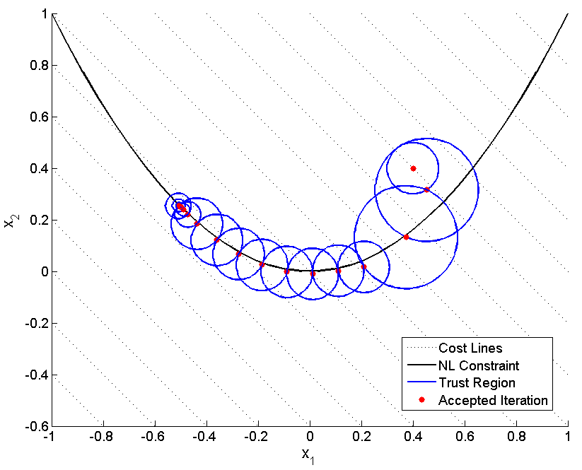
Figure 1: Typical convergence process with virtual control and trust regions.

II-B4 The SCvx Algorithm

The final problem formulation and the SCvx algorithm can now be presented. Considering the virtual control and the trust regions, a Convex Optimal Control Problem (COCP) is solved at $k^{th}$ succession:

Problem 2 (COCP).

Determine $w^{*}\in L_{\infty}[0,T]^{m}$, and $d^{*}\in W_{1,\infty}[0,T]^{n}$, which minimize the functional $L(d,w)$ defined in (5), subject to constraints (4), (7), as well as

$$u^{k}(t)+w(t) \in U,$$

$$x^{k}(t)+d(t) \in X.$$

With this convex subproblem, SCvx algorithm is given as in Algorithm 1.

Algorithm 1 Successive Convexification (SCvx)

  Input Select initial state $x^{1}$ and control $u^{1}$ s.t. $x^{1}\in X$ and $u^{1}\in U$. Initialize trust region radius with positive $\varDelta^{1}$ and lower bound $\varDelta_{l}$. Select positive penalty weight $\lambda$, and parameters $0<\rho_{0}<\rho_{1}<\rho_{2}<1$ and $\alpha>1$.

  Step 1 At each succession $k$, solve Problem 2 at $(x^{k},u^{k},\varDelta^{k})$ to get an optimal solution $d^{k}$.

  Step 2 Compute the ”actual” change in the penalized cost (6):

$$\Delta J(x^{k},u^{k})\coloneqq\Delta J^{k}=J(x^{k},u^{k})-J(x^{k}+d^{k},u^{k}+w^{k}),$$ (8)

and the ”predicted” change by linear approximation:

$$\Delta L(d^{k},w^{k})\coloneqq\Delta L^{k}=J(x^{k},u^{k})-L(d^{k},w^{k}).$$ (9)

  if $\Delta L^{k}=0$ then

     Stop, and return $(x^{k},u^{k})$;

  else

     Compute the ratio $r^{k}=\Delta J^{k}/\Delta L^{k}$.

  end if

  Step 3

  if $r^{k}<\rho_{0}$ then

     Reject this step, contract the trust region radius, i.e. $\varDelta_{k}\leftarrow\varDelta_{k}/\alpha$ and go back to Step 1;

  else

     Accept this step, i.e. $x^{k+1}\leftarrow x^{k}+d^{k}$, $u^{k+1}\leftarrow u^{k}+w^{k}$, and update $\varDelta^{k+1}$ by

$$\varDelta^{k+1}=\begin{cases}\varDelta^{k}/\alpha,&\text{if }r^{k}<\rho_{1};\\ \varDelta^{k},&\text{if }\rho_{1}\leq r^{k}<\rho_{2};\\ \alpha\varDelta^{k},&\text{if }\rho_{2}\leq r^{k}.\end{cases}$$

  end if

  $\varDelta^{k+1}\leftarrow\max\{\varDelta^{k+1},\varDelta_{l}\}$, $k\leftarrow k+1$, and go to Step 1.

This algorithm is of trust region type, and follows standard trust region radius update rules with some modifications.

One important distinction lies in the subproblem to be solved at each succession. Conventional trust region algorithms usually perform a line search along the Cauchy arc to achieve a ”sufficient” reduction [24]. In our algorithms, however, a full convex optimization problem is solved to speed up the process, i.e. we solve the subproblem to its full optimality. As a result, the number of successions can be significantly less, by achieving more cost reduction at each succession. Admittedly, computational effort may slightly increase at each succession, but thanks to the algorithm customization techniques [11], we are able to solve each convex subproblem fast enough to outweigh the negative impact of solving it to full optimality.

In Step 2, the ratio $r^{k}$ is used as a metric for the quality of linear approximations. A desirable scenario is when $\Delta J^{k}$ agrees with $\Delta L^{k}$, i.e. $r^{k}$ is close to 1. Hence if $r^{k}$ is above $\rho_{2}$, which means our linear approximation predicts the cost reduction well, then we may choose to enlarge the trust region in Step 3, i.e., we put more faith in our approximation. Otherwise, we may keep the trust region unchanged, or contract its radius if needed. The most unwanted situation is when $r^{k}$ is negative, or close to zero. The current step will be rejected in this case, and one has to contract the trust region and re-optimize at $(x^{k},u^{k})$.

III CONVERGENCE ANALYSIS

In this section, we present a convergence analysis in the continuous-time setting. Hence we re-formulate the continuous-time optimal control problem as an infinite dimensional optimization problem in Banach space to simplify notations. To do this, we treat both the states and the control as independent variables, so that in Problem 1 and Problem 2, (2b) and (4) are considered as equality constraints. For simplicity, we denote our variable pair $(x,u)$ as $x$ in the sequel. Thus the space X will be re-defined as

$$X\coloneqq W_{1,\infty}[0,T]^{n}\times L_{\infty}[0,T]^{m}.$$

Following this definition, the original dynamics will be represented by a set of algebraic equations:

$$g_{i}(x)=0,\quad i=1,2,\ldots,n,$$ (10)

and the original state and control constraints will be represented by a set of inequalities:

$$h_{j}(x)\leq 0,\quad j=1,2,\ldots,n+m.$$ (11)

Denote the set of $x$ satisfying (11) as $F$,

$$F=\{x\,|\,h_{j}(x)\leq 0,\quad j=1,2,\ldots,n+m\}.$$ (12)

For objective functional, the original one (2a) becomes

$$\Psi(x)\coloneqq\varphi(x(T),T)+\int_{0}^{T}L(x(t),t)\;dt.$$ (13)

Note that $\Psi(\cdot)$ is Fréchet differentiable, since $\varphi(\cdot)$ and $L(\cdot)$ are both differentiable. Now Problem 1 is ready to be re-formulated as:

Problem 3.

Determine $x\in X$, which minimizes $\Psi(x)$ defined in (13), subject to constraints (10) and (11).

If we rewrite (10) in a more concise form, $g(x)=0$, then the penalized cost defined in (6) will be

$$J(x,\lambda)\coloneqq\Psi(x)+\lambda\gamma(g(x)).$$ (14)

Then the associated penalty problem can be established in a similar manner:

Problem 4.

Determine $x\in X$, which minimizes $J(x,\lambda)$ defined in (14), subject to constraints (11).

III-A Exactness of Penalty Function $\gamma(g(x))$

We say a penalty function is exact, if there exists a finite $\lambda$ such that problems before and after penalizing are equivalent in the sense of optimality conditions. A geometric justification of exactness for $\gamma(g(x))$ with different norms can be found in [22]. Alternatively, we can also show it via analysis. To do this, we need to introduce some definitions and assumptions first.

Definition 1 (Local Optimum).

If there exist $\bar{\lambda}\geq 0$ and $\bar{x}\in F$ such that $J(\bar{x},\lambda)\leq J(x,\lambda)$ for all $\lambda\geq\bar{\lambda}$ and for all $x\in N(\bar{x})\cap F$, where $N(\bar{x})$ denotes an open neighborhood of $\bar{x}$, then $\bar{x}$ is a local optimum of Problem 3.

Assumption 1 (LICQ).

Linear Independence Constraint Qualification (LICQ) is satisfied at $\bar{x}$ if the gradients of active constraints

$$\{\,\nabla g_{1}(\bar{x}),\ldots,\nabla g_{n}(\bar{x});\nabla h_{i}(\bar{x}),i\in I(\bar{x})\,\}$$

are linearly independent, where $I(\bar{x})$ is the index set of active inequality constraints,

$$I(\bar{x})=\{i\,|\,h_{i}(\bar{x})=0,\quad i=1,2,\ldots,n+m\}.$$

Now we are ready to present our first theorem, which states the stationarity part of the first order necessary conditions (KKT conditions) for a point $\bar{x}$ to be a local solution of Problem 3, as in Definition 1.

Theorem 1 (Stationary Conditions).

If the nonlinear constraints of Problem 3 satisfy LICQ, and $\bar{x}$ is a local solution of Problem 3, then there exist Lagrange multipliers $\mu_{i}$ and $\sigma_{i}\geq 0$ such that

$$\nabla\Psi(\bar{x})+\operatorname*{ess\,sup}\limits_{t\in[0,T]}\sum_{i=1}^{n}\mu_{i}\nabla g_{i}(\bar{x})+\sum_{i\in I(\bar{x})}\sigma_{i}\nabla h_{i}(\bar{x})=0.$$

Proof.

It directly follows Corollary 1 in [25], with some minor modifications to facilitate the essential supremum, $\operatorname*{ess\,sup}\limits_{t\in[0,T]}(\cdot)$. ∎

An equivalent form of Theorem 1 is Theorem 3.11 from [21], which involves a Hamiltonian and is interpreted as a local minimum principle.

To examine the exactness of $\gamma(g(x))$, we also need to establish optimality conditions for the penalty problem, i.e. Problem 4. For fixed $\lambda$, the cost $J(x)$ is not differentiable everywhere due to non-smoothness of $\gamma(g(x))$. However, since $\Psi(x)$ and $g(x)$ are both continuously Fréchet differentiable, $J$ is locally Lipschitz continuous. Then we have

Definition 2 (GDD).

If $J$ is locally Lipschitz continuous, the Generalized Directional Derivative (GDD) of $J$ at $\bar{x}$ in any direction s exists, and can be defined as

$$dJ(\bar{x},s)\coloneqq\limsup\limits_{\mathclap{\begin{subarray}{c}x\rightarrow\bar{x}\\ \delta\rightarrow 0^{+}\end{subarray}}}\frac{J(x+\delta s)-J(x)}{\delta}.$$ (15)

By [26], $dJ$ as defined above also satisfies the following implicit relationship,

$$dJ(\bar{x},s)=\max\{\langle\nu,s\rangle\,|\,\nu\in\partial J(\bar{x})\},$$ (16)

where $\partial J(\bar{x})$ is the generalized differential of $J$ at $\bar{x}$, i.e.

$$\partial J(\bar{x})=\{\nu\,|\,dJ(\bar{x},y)\geq\nu y,\forall y\in X\}.$$ (17)

Applying Theorem 1 in [25] and Using the above definitions, we have

Lemma 1.

If $\bar{x}$ is a local solution of Problem 4, then there exist multipliers $\sigma_{i}\geq 0$ such that

$$0\in\partial J(\bar{x})+\left\{y\,|\,y=\sum_{i\in I(\bar{x})}\sigma_{i}\nabla h_{i}(\bar{x})\right\}\triangleq D(\bar{x}),$$ (18)

where the ”$+$” sign stands for the Minkowski sum of two sets.

Define the set of constrained stationary points of Problem 4 as

$$S\coloneqq\{x\,|\,x\in F\text{ and }0\in D(x)\}.$$

Lemma 1 states that if $\bar{x}$ solves Problem 4, then $\bar{x}\in S$.

Next lemma gives an explicit expression of $\partial J(x)$ for any $x$ and directly follows Theorem 2.1 in [27].

Lemma 2.

For any fixed positive weight $\lambda$, the generalized differential of the penalized cost $J(x)$ is

$$\partial J(x)=\left\{\nabla\Psi(x)+\lambda\operatorname*{ess\,sup}\limits_{t\in[0,T]}\sum_{i=1}^{n}\mu_{i}\nabla g_{i}(x)\,|\,\mu_{i}\right\}$$

where $\mu_{i}$ is defined by

$$\mu_{i}\begin{cases}=\text{sgn }g_{i}(x),&\text{if }g_{i}(x)\neq 0;\\ \in[-1,1],&\text{if }g_{i}(x)=0.\end{cases}$$

Next theorem gives the main result in this subsection, that is, the exactness of the penalty problem.

Theorem 2.

If $\bar{x}$ is a stationary point of Problem 3 with multipliers $\bar{\mu}_{i}$, and $\bar{\sigma}_{i}$, and if penalty weight $\lambda$ satisfies

$$\lambda\geq|\bar{\mu}_{i}|,\quad\forall\;i=1,2,\ldots,n,$$ (19)

then $\bar{x}$ is a constrained stationary point of Problem 4, that is, $\bar{x}\in S$.

Conversely, if $\bar{x}\in S$ is feasible for Problem 3, then it is a stationary point of Problem 3.

Proof.

From Theorem 1, we have

$$\nabla\Psi(\bar{x})+\operatorname*{ess\,sup}\limits_{t\in[0,T]}\sum_{i=1}^{n}\bar{\mu_{i}}\nabla g_{i}(\bar{x})+\sum_{i\in I(\bar{x})}\bar{\sigma_{i}}\nabla h_{i}(\bar{x})=0,$$ (20)

and $\bar{\sigma_{i}}\geq 0$. Since $\bar{x}$ is feasible to Problem 3, we have $g_{i}(\bar{x})=0$. Therefore from Lemma 2, the generalized differential at $\bar{x}$ is

$$\partial J(\bar{x})=\left\{\nabla\Psi(\bar{x})+\lambda\operatorname*{ess\,sup}\limits_{t\in[0,T]}\sum_{i=1}^{n}\mu_{i}\nabla g_{i}(\bar{x})\,|\,\mu_{i}\right\},$$

where $\mu_{i}\in[-1,1]$. Then from (19), $\lambda\geq 1$. Hence $\lambda\mu_{i}$ can take any value in $\mathbb{R}$, including $\bar{\mu_{i}}$. In other words,

$$\nabla\Psi(\bar{x})+\operatorname*{ess\,sup}\limits_{t\in[0,T]}\sum_{i=1}^{n}\bar{\mu_{i}}\nabla g_{i}(\bar{x})\in\partial J(\bar{x}).$$

Combining this with $\bar{\sigma_{i}}\geq 0$, from (20) we have $0\in D(\bar{x})$, which has been defined in (18). Again, since $\bar{x}$ is feasible, $\bar{x}\in F$, i.e. $\bar{x}\in S$.

Converse result can be trivially derived from Lemma 1 and Lemma 2. ∎

Remark.

Although Theorem 2 does not suggest a constructive way to find such a $\lambda$, it still has important theoretical values. In our current implementations, we select a ”sufficiently” large $\lambda$ and keep it fixed for the whole process. Numerical results show that this works well for most applications.

The ”conversely” part of Theorem 2 is what really matters to our subsequent convergence analysis. It guarantees that as long as we can find a stationary point for the penalty problem which is feasible to the original problem, we reach stationarity of the original problem as well.

III-B Convergence Analysis

Two major convergence results will be stated in this subsection. The first one deals with the case of finite convergence, while the second will handle the situation where an infinite sequence $\{x^{k}\}$ is generated by the SCvx algorithm. Note that for simplicity, we suppress the dependence on control variables $u$ and $w$ in $J$ and $L$ respectively, i.e. $x$ means $(x,u)$ and $d$ stands for $(d,w)$. For the finite case, we have

Theorem 3.

The ”predicted” changes $\Delta L^{k}$ defined in (9) are nonnegative for any $k$. Furthermore, $\Delta L^{k}=0$ implies that $x^{k}$ is a stationary point of Problem 4, i.e. $x^{k}\in S$.

Proof.

$d=0$ is always feasible for the convex subproblem, Problem 2, while $d^{k}$ solves this problem. Hence we have

$$L(d^{k})\leq L(0)=J(x^{k}),$$

so that $\Delta L^{k}=J(x^{k})-L(d^{k})\geq 0$, and $\Delta L^{k}=0$ if and only if $d=0$ solves problem 2. In the $\Delta L^{k}=0$ case, one can directly apply Lemma 1 and Lemma 2 to get $x^{k}\in S$. ∎

Now the real challenge is when $\{x^{k}\}$ is an infinite sequence. It would be nice to have some smoothness when examining the limit process. However in this case, the non-differentiable penalty function $\gamma(\cdot)$ poses difficulties to our analysis. To facilitate further results, we first note that for any $x$,

$$J(x+d)=L(d)+o(\|d\|)$$ (21)

and $o(\|d\|)$ is independent of $x$. This can be verified by simply writing out the Taylor expansion of $J(x)$ and using the fact that $\gamma(\cdot)$ is a linear operator.

Next lemma is the major preliminary result, and its proof also provides some geometric insights of the SCvx algorithm we described.

Lemma 3.

Let $\bar{x}\in F$ but $\bar{x}\notin S$, i,e, $\bar{x}$ is feasible but not a stationary point of the penalty problem, and any scalar $c\leq 1$. Then there exist positive $\bar{\varDelta}$ and $\bar{\epsilon}$ such that for all $x\in N(\bar{x},\bar{\epsilon})\cap F$ and $0<\varDelta\leq\bar{\varDelta}$, any optimal solution $\bar{d}$ of the convex subproblem, Problem 2 solved at $x$ with trust region radius $\varDelta$ satisfies

$$r(x,\varDelta)=\frac{J(x)-J(x+\bar{d})}{J(x)-L(\bar{d})}\geq c,$$ (22)

where $N(\bar{x},\bar{\epsilon})$ represents an open neighborhood of $\bar{x}$ with radius $\bar{\epsilon}$.

Proof.

Since $\bar{x}\in F$ but $\bar{x}\notin S$, we know that $0\notin D(\bar{x})$, where $D(\bar{x})$ is defined in (18).

By definition in (17), the generalized differential $\partial J(\bar{x})$ is the intersection of half spaces, and hence it is a closed convex set. Also, the set

$$\left\{y\,|\,y=\sum_{i\in I(\bar{x})}\sigma_{i}\nabla h_{i}(\bar{x}),\;\text{for some }\sigma_{i}\geq 0\right\}\triangleq C(\bar{x})$$ (23)

is a conic combination of $\nabla h_{i}(\bar{x})$, hence it is a closed convex cone. Since Minkowski sum preserves convexity, $D(\bar{x})$ is a closed and convex set as well. Applying the separation theorem of convex sets to $D(\bar{x})$, we get that there exists a unit vector $s$ and a scalar $\kappa>0$ such that for all $\nu\in D(\bar{x})$,

$$\langle\nu,s\rangle\leq-\kappa<0.$$ (24)

Since $\partial J(\bar{x})$ is a subset of $D(\bar{x})$, (24) holds for all $\nu\in\partial J(\bar{x})$, which means $\max\{\langle\nu,s\rangle\,|\,\nu\in\partial J(\bar{x})\}\leq-\kappa$. The left hand side is exactly the expression for GDD as described in (16). Therefore, we have

$$dJ(\bar{x},s)\coloneqq\limsup\limits_{\mathclap{\begin{subarray}{c}x\rightarrow\bar{x}\\ \varDelta\rightarrow 0^{+}\end{subarray}}}\frac{J(x+\varDelta s)-J(x)}{\varDelta}\leq-\kappa.$$

It implies that there exist positive $\bar{\varDelta}$ and $\bar{\epsilon}$ such that for all $x\in N(\bar{x},\bar{\epsilon})\cap F$ and $0<\varDelta\leq\bar{\varDelta}$,

$$\frac{J(x+\varDelta s)-J(x)}{\varDelta}<-\frac{\kappa}{2}.$$ (25)

Another subset of $D(\bar{x})$ is $C(\bar{x})$ defined in (23), so (24) also holds for all $\nu\in C(\bar{x})$. This necessarily implies

$$\langle\nabla h_{i}(\bar{x}),s\rangle\leq 0,\quad i\in I(\bar{x}),$$ (26)

which essentially means $s$ is a feasible direction of the active constraints at $\bar{x}$.

Now consider Problem 2 is solved with such $x$ and $\varDelta$, and gives an optimal solution $\bar{d}$. By using (21), the ”actual” change in $J$ is

$$\Delta J(x,\bar{d}) =J(x)-J(x+\bar{d})$$

$$=J(x)-L(\bar{d})-o(\|\bar{d}\|)$$

$$=\Delta L(\bar{d})-o(\|\varDelta\|).$$ (27)

Thus the ratio

$$r(x,\varDelta)=\frac{\Delta J(x,\bar{d})}{\Delta L(\bar{d})}=1-\frac{o(\|\varDelta\|)}{\Delta L(\bar{d})}.$$

Let $d^{\prime}=\varDelta s$. Since $s$ is a feasible direction as implied by (26), $d^{\prime}$ will be a feasible solution to Problem 2, while $\bar{d}$ is optimal. Thus we have $L(\bar{d})\leq L(d^{\prime})$, which in turn means

$$\Delta L(\bar{d})\geq\Delta L(d^{\prime})$$ (28)

Now in the $\varDelta\rightarrow 0$ process, $0<\varDelta\leq\bar{\varDelta}$ will be satisfied. Then from (25), we have

$$\Delta J(x,d^{\prime})=J(x)-J(x+d^{\prime})>\left(\frac{\kappa}{2}\right)\varDelta.$$

With $\bar{d}$ replaced by $d^{\prime}$ in (27),

$$\Delta J(x,d^{\prime})=\Delta L(d^{\prime})-o(\|\varDelta\|)\geq\left(\frac{\kappa}{2}\right)\varDelta.$$

Combining this with (28), we get

$$\Delta L(x,\bar{d})\geq\Delta L(d^{\prime})-o(\|\varDelta\|)>\left(\frac{\kappa}{2}\right)\varDelta.$$

Thus $\Delta L(x,\bar{d})>(\kappa/2)\varDelta+o(\|\varDelta\|)$, and the ratio

$$r(x,\varDelta)=1-\frac{o(\|\varDelta\|)}{\Delta L(\bar{d})}>1-\frac{o(\|\varDelta\|)}{(\kappa/2)\varDelta+o(\|\varDelta\|)}.$$

Therefore, as $\varDelta\rightarrow 0$, $r(x,\varDelta)\rightarrow 1$, and thus for any $c<1$, $r(x,\varDelta)\geq c$. ∎

Remark.

A frustrating situation happens when the algorithm keeps rejecting our trial steps. Fortunately, Lemma 3 provides some assurance that the SCvx algorithm won’t reject the trial steps forever. At some point, usually after reducing $\varDelta^{k}$ several times, the ratio metric $r^{k}$ will be greater than any prescribed $c$, hence $r^{k}\geq\rho_{0}$ is guaranteed.

We can now present our main result in this section.

Theorem 4.

If the SCvx algorithm generates an infinite sequence $\{x^{k}\}$, then $\{x^{k}\}$ has limit points, and any limit point $\bar{x}$ is a constrained stationary point of Problem 4, i.e. $\bar{x}\in S$.

Proof.

The proof is by contradiction. Since we have assumed the feasible region to be convex and compact, there is at least one subsequence $\{x^{k_{i}}\}\rightarrow\bar{x}$, which is NOT a stationary point. From Lemma 3, there exist positive $\bar{\varDelta}$ and $\bar{\epsilon}$ such that

$$r(x,\varDelta)\geq\rho_{0}\quad\text{for all }x\in N(\bar{x},\bar{\epsilon})\cap F\text{ and }0<\varDelta\leq\bar{\varDelta}.$$

Without loss of generality, we can suppose the whole subsequence $\{x^{k_{i}}\}$ is in $N(\bar{x},\bar{\epsilon})$, so

$$r(x^{k_{i}},\varDelta)\geq\rho_{0}\quad\text{for all }0<\varDelta\leq\bar{\varDelta}.$$ (29)

If the initial trust region radius is less than $\bar{\varDelta}$, then (29) will be trivially satisfied.

Now if the initial radius is greater than $\bar{\varDelta}$, then $\varDelta$ may need to be reduced several times before the condition (29) is met. Let $\hat{\varDelta}$ be the last $\varDelta^{k_{i}}$ that needs to be reduced, then evidently $\hat{\varDelta}>\bar{\varDelta}$. Also, let $\varDelta^{k_{i}}$ be the subsequence consists of all the valid radius after the last rejection. Then

$$\varDelta^{k_{i}}=\hat{\varDelta}/\alpha>\bar{\varDelta}/\alpha.$$

Since there is also a lower bound $\varDelta_{l}$ on $\varDelta$, we have

$$\varDelta^{k_{i}}\geq\min\{\varDelta_{l},\bar{\varDelta}/\alpha\}\triangleq\delta.$$ (30)

Note that condition (29) can be express as

$$J(x^{k_{i}})-J(x^{k_{i}+1})\geq\rho_{0}\Delta L^{k_{i}}.$$ (31)

Our next goal is to find a lower bound for $\Delta L^{k_{i}}$. Further, we let $\bar{d}$ solves the convex subproblem, Problem 2 at $\bar{x}$ with trust region radius $\delta/2$, i.e. $\|\bar{d}\|_{\infty}\leq\delta/2$. Let $\hat{x}=\bar{x}+\bar{d}$, then

$$\|\hat{x}-\bar{x}\|_{\infty}\leq\delta/2.$$ (32)

Since $\bar{x}\notin S$, Theorem 3 implies

$$\Delta L(\bar{d})=J(\bar{x})-L(\bar{d})\triangleq\theta>0.$$

By continuity of $J$ and $L$, there exists an $i_{0}>0$ such that for all $i\geq i_{0}$

$$J(x^{k_{i}})-L(\hat{x}-x^{k_{i}})>\theta/2,\text{ and}$$ (33)

$$\|x^{k_{i}}-\bar{x}\|_{\infty}<\delta/2.$$ (34)

From (32) and (34), we have for all $i\geq i_{0}$

$$\|\hat{x}-x^{k_{i}}\|_{\infty}\leq\|\hat{x}-\bar{x}\|_{\infty}+\|x^{k_{i}}-\bar{x}\|_{\infty}<\delta\leq\varDelta^{k_{i}}.$$ (35)

where the last inequality comes from (30). Let $\hat{d}^{k_{i}}=\hat{x}-x^{k_{i}}$, (35) implies $\hat{d}^{k_{i}}$ is a feasible solution for the convex subproblem at $(x^{k_{i}},\varDelta^{k_{i}})$ when $i\geq i_{0}$. Then if $d^{k_{i}}$ is the optimal solution to this subproblem, we have $L(d^{k_{i}})\leq L(\hat{d}^{k_{i}})$, so

$$\Delta L(d^{k_{i}})=J(x^{k_{i}})-L(d^{k_{i}})\geq J(x^{k_{i}})-L(\hat{d}^{k_{i}})>\theta/2.$$ (36)

The last inequality is due to (33). Combine (31) and (36), we have for all $i\geq i_{0}$

$$J(x^{k_{i}})-J(x^{k_{i}+1})\geq\rho_{0}\theta/2.$$ (37)

However, the positive infinite series

$$\sum_{i=1}^{\infty}\left(J(x^{k_{i}})-J(x^{k_{i}+1})\right) \leq\sum_{i=1}^{\infty}\left(J(x^{k_{i}})-J(x^{k_{i+1}})\right)$$

$$=J(x^{k_{1}})-J(\bar{(}x))\leq\infty.$$

Thus it is convergent, so necessarily

$$J(x^{k_{i}})-J(x^{k_{i}+1})\;\rightarrow\;0,$$

which contradicts (37). Therefore, we conclude that every limit point $\bar{x}\in S$. ∎

IV NUMERICAL SIMULATIONS

This section presents a numerical example to demonstrate the proposed algorithm’s capabilities. The example consists of a mass subject to “double-integrator” dynamics with nonlinear aerodynamic drag. The mass is controlled using a thrust input, $\mathbf{T}$, that is limited to a maximum magnitude of $T_{max}$. The problem formulation is summarized below, and its parameters are given in Table LABEL:t:sim_params.

minimize $$\int_{0}^{t_{f}}{\Gamma(\tau)d\tau}\quad\text{s.t.}$$

$$\mathbf{x}(0) =\mathbf{x}_{i}\quad\quad\,\ \mathbf{v}(0)=\mathbf{v}_{i}$$

$$\mathbf{x}(t_{f}) =\mathbf{x}_{f}\quad\quad\mathbf{v}(t_{f})=\mathbf{v}_{f}$$

$$\dot{\mathbf{x}}(t) =\mathbf{v}(t)\quad\;\;\;\dot{\mathbf{v}}(t)=\mathbf{a}(t)$$

$$\mathbf{a}(t) =\frac{1}{m}\left(\mathbf{T}(t)-k_{d}||\mathbf{v}(t)||\mathbf{v}(t)\right)$$

$$||\mathbf{T}(t)|| \leq\Gamma(t)\leq T_{max}.$$

TABLE I: Simulation Parameters

Parameter	Value
$t_{f}$	10
$m$	1.0
$k_{d}$	0.25
$T_{max}$	2.0
$\mathbf{x}_{i}$	$[0\quad 0]^{T}$
$\mathbf{x}_{f}$	$[10\quad 10]^{T}$
$\mathbf{v}_{i}$	$[5\quad 0]^{T}$
$\mathbf{v}_{f}$	$[5\quad 0]^{T}$
$\Delta_{l}$	$0.0$
$\rho_{0}$	$0.0$
$\rho_{1}$	$0.25$
$\rho_{2}$	$0.9$
$\alpha$	$2.0$

Here, we linearize the first succession about a constant velocity straight-line trajectory from the initial to the final position. The convergence history is presented in Fig. 2, where the first 10 accepted successions are shown, after which a desirable convergence is achieved.

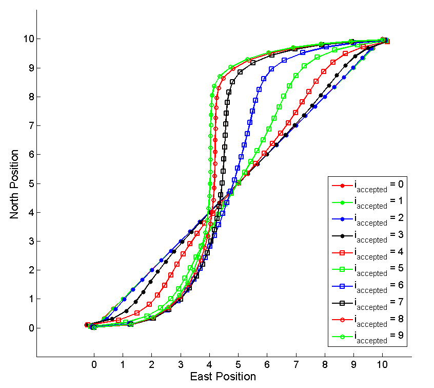
Figure 2: Convergence history of two-dimensional trajectory. The dots along the trajectory indicate time-discretization points.

Fig. 3 shows the converged thrust magnitude profile. The plot also shows a no-drag thrust magnitude profile for the same scenario. Note that the no-drag case renders the problem convex, thus recovering the classical “bang-bang” solution. In contrast, the case with aerodynamic drag takes advantage of drag at the beginning by decreasing its thrust magnitude, and must sustain a non-zero thrust in the middle of the trajectory to counter the energy loss induced by drag. Note that the area under the thrust curve in the case with drag is less than that of the case without drag. Thus, we see evidence of a situation where the optimal cost of the problem is reduced due to the inclusion of nonlinear dynamics.

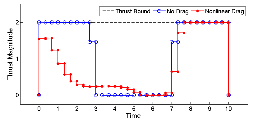
Figure 3: Convergence history of solution and thrust profile: The thrust magnitude profile of the converged solution (red) and of the corresponding no-drag problem (blue). The markers indicate time-discretization points.

Fig. 4 show the process the algorithm undergoes in obtaining the solution. The top plot shows how $r^{k}$ varies as a function of iteration number, and how the trial step is rejected when $r^{k}$ drops below $\rho_{0}$. Note that the trust region radius increases whenever $r^{k}$ is greater than $\rho_{2}$, stays the same when $\rho_{1}\leq r^{k}\leq\rho_{2}$ or $r^{k}\leq\rho_{0}$, and decreases when $\rho_{0}\leq r^{k}\leq\rho_{1}$. More importantly, we can see how the process of rejecting the step results in decreasing the trust region radius, $\Delta^{k}$, thus increasing $r^{k}$ back above $\rho_{0}$.

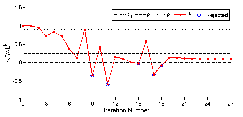
Figure 4: Algorithm behavior during the solution process. The plot shows the time history of $r^{k}$ relative to the thresholds $\rho_{0}$, $\rho_{1}$, and $\rho_{2}$, and indicates the rejected steps.

V CONCLUSIONS

In this paper, we have proposed the SCvx algorithms. It successively convexifies nonlinear dynamics, and enables us to solve non-convex optimal control problems in real-time by actually solving a sequence of convex subproblem. We have given a relatively thorough description and analysis of the proposed algorithm, with the aid of a simple, yet illustrative numerical example. Convergence has been demonstrated in theoretical proofs, as well as illustrative figures and plots. The main result is: for the infinite convergent case, we have proved that every limit point will satisfied the optimality condition for the original non-convex optimal control problems. A key next step is to incorporate this algorithm with other convexification techniques to construct a comprehensive algorithmic framework to deal with a large class of non-convexities.

Acknowledgments

The authors gratefully acknowledge John Hauser of University of Colorado for his deep and valuable insights.

References

- [1] B. Açıkmeşe, J. Carson, and L. Blackmore, “Lossless convexification of non-convex control bound and pointing constraints of the soft landing optimal control problem,” IEEE Transactions on Control Systems Technology, vol. 21, no. 6, pp. 2104–2113, 2013.
- [2] L. Blackmore, B. Açıkmeşe, and J. M. Carson, “Lossless convexfication of control constraints for a class of nonlinear optimal control problems,” System and Control Letters, vol. 61, no. 4, pp. 863–871, 2012.
- [3] A. Richards, T. Schouwenaars, J. P. How, and E. Feron, “Spacecraft trajectory planning with avoidance constraints using mixed-integer linear programming,” Journal of Guidance, Control, and Dynamics, vol. 25, no. 4, pp. 755–764, 2002.
- [4] X. Liu and P. Lu, “Solving nonconvex optimal control problems by convex optimization,” Journal of Guidance, Control, and Dynamics, vol. 37, no. 3, pp. 750–765, 2014.
- [5] C. Buskens and H. Maurer, “Sqp-methods for solving optimal control problems with control and state constraints: adjoint variables, sensitivity analysis, and real-time control,” Journal of Computational and Applied Mathematics, vol. 120, pp. 85–108, 2000.
- [6] M. Gerdts, “A nonsmooth newtom’s method for control-state constrained optimal control problems,” Mathematics and Computers in Simulation, 2008.
- [7] D. Hull, “Conversion of optimal control problems into parameter optimization problems,” Journal of Guidance, Control, and Dynamics, vol. 20, no. 1, pp. 57–60, 1997.
- [8] S. Boyd and L. Vandenberghe, Convex Optimization. Cambridge University Press, 2004.
- [9] A. Domahidi, E. Chu, and S. Boyd, “ECOS: An SOCP solver for Embedded Systems,” in Proceedings European Control Conference, 2013.
- [10] J. Mattingley and S. Boyd, “Cvxgen: A code generator for embedded convex optimization,” Optimization and Engineering, vol. 13, no. 1, pp. 1–27, 2012.
- [11] D. Dueri, J. Zhang, and B. Açikmese, “Automated custom code generation for embedded, real-time second order cone programming,” in 19th IFAC World Congress, 2014, pp. 1605–1612.
- [12] C. Garcia and M. Morari, “Model predictive control: theory and practice — a survey,” Automatica, vol. 25, no. 3, pp. 335–348, 1989.
- [13] D. Mayne, J. Rawlings, C. Rao, and P. Scokaert, “Constrained model predictive control: Stability and optimality,” Automatica, vol. 36, no. 6, pp. 789–814, 2000.
- [14] M. N. Zeilinger, D. M. Raimondo, A. Domahidi, M. Morari, and C. N. Jones, “On real-time robust model predictive control,” Automatica, vol. 50, no. 3, pp. 683 – 694, 2014.
- [15] M. Harris and B. Açıkmeşe, “Lossless convexification of non-convex optimal control problems for state constrained linear systems,” Automatica, vol. 50, no. 9, pp. 2304–2311, 2014.
- [16] B. Açıkmeşe and L. Blackmore, “Lossless convexification of a class of optimal control problems with non-convex control constraints,” Automatica, vol. 47, no. 2, pp. 341–347, 2011.
- [17] R. E. Griffith and R. Stewart, “A nonlinear programming technique for the optimization of continuous processing systems,” Management science, vol. 7, no. 4, pp. 379–392, 1961.
- [18] F. Palacios-Gomez, L. Lasdon, and M. Engquist, “Nonlinear optimization by successive linear programming,” Management Science, vol. 28, no. 10, pp. 1106–1120, 1982.
- [19] J. Zhang, N.-H. Kim, and L. Lasdon, “An improved successive linear programming algorithm,” Management science, vol. 31, no. 10, pp. 1312–1331, 1985.
- [20] J. B. Rosen, “Iterative solution of nonlinear optimal control problems,” SIAM Journal on Control, vol. 4, no. 1, pp. 223–244, 1966.
- [21] K. C. P. Machielsen, Numerical solution of optimal control problems with state constraints by sequential quadratic programming in function space. Technische Universiteit Eindhoven, 1987.
- [22] D. Q. Mayne and E. Polak, “An exact penalty function algorithm for control problems with state and control constraints,” Automatic Control, IEEE Transactions on, vol. 32, no. 5, pp. 380–387, 1987.
- [23] S.-P. Han and O. L. Mangasarian, “Exact penalty functions in nonlinear programming,” Mathematical programming, vol. 17, no. 1, pp. 251–269, 1979.
- [24] A. R. Conn, N. I. Gould, and P. L. Toint, Trust region methods. Siam, 2000, vol. 1.
- [25] F. H. Clarke, “A new approach to lagrange multipliers,” Mathematics of Operations Research, vol. 1, no. 2, pp. 165–174, 1976.
- [26] R. Fletcher, Practical Methods of Optimization: Vol. 2: Constrained Optimization. John Wiley & Sons, 1981.
- [27] F. H. Clarke, “Generalized gradients and applications,” Transactions of the American Mathematical Society, vol. 205, pp. 247–262, 1975.