Herschel/PACS far-IR spectral imaging of a jet from an intermediate mass protostar in the OMC-2 region

We present the first detection of a jet in the far-IR [O I] lines from an intermediate mass protostar. We have carried out a Herschel/PACS spectral mapping study in the [O I] lines of OMC-2 FIR 3 and FIR 4, two of the most luminous protostars in Orion outside of the Orion Nebula. The spatial morphology of the fine structure line emission reveals the presence of an extended photodissociation region (PDR) and a narrow, but intense jet connecting the two protostars. The jet seen in [O I] emission is spatially aligned with the Spitzer/IRAC 4.5 $\mu\mathrm{m}$ jet and the CO (6-5) molecular outflow centered on FIR 3. The mass loss rate derived from the total [O I] 63 $\mu\mathrm{m}$ line luminosity of the jet is 7.7 $\times$10^-6 M_⊙ yr^-1, more than an order of magnitude higher than that measured for typical low mass class 0 protostars. The implied accretion luminosity is significantly higher than the observed bolometric luminosity of FIR 4, indicating that the [O I] jet is unlikely to be associated with FIR 4. We argue that the peak line emission seen toward FIR 4 originates in the terminal shock produced by the jet driven by FIR 3. The higher mass-loss rate that we find for FIR 3 is consistent with the idea that intermediate mass protostars drive more powerful jets than their low-mass counterparts. Our results also call into question the nature of FIR 4.

1 Introduction

The far-infrared lines of [O I] are prominent tracers of jets from young stars and protostars. They provide a straightforward measure of the mass flow through dissociative J-shocks driven by the outflowing jets (Werner et al. 1984; Cohen et al. 1988; Nisini et al. 1996; Hollenbach 1985; Hollenbach & McKee 1989). In regions of high extinction, as those found around young protostars, [O I] lines are a means to trace and characterize jets from outflows, unaffected by extinction or confusion with the ambient molecular cloud. While [O I] jets from optically revealed pre-main sequence stars and low-mafss protostars have been detected with Herschel/PACS (e.g., Podio et al. 2012; Nisini et al. 2015), no such detections have been reported for embedded intermediate mass protostars.

Table 1: Log of PACS spectroscopic observations

HOPS ID	ObsID	OD	Date	Total time	RA	DEC	Observing mode	Spectral range
				(s)	($\deg$)	($\deg$)
FIR 3 (OFF)	1342227763	838	2011 Aug 30	989	5 32 18.750	$-$6 24 27.50	pointed	57-71 $\&$170-213
FIR 3 (ON)	1342227764	838	2011 Aug 30	8933	5 35 27.670	$-$5 09 35.10	$3\times 3$ raster	57-71 $\&$170-213
FIR 3 (OFF)	1342227765	838	2011 Aug 30	989	5 32 18.750	$-$6 24 27.50	pointed	57-71 $\&$170-213
FIR 3 (ON)	1342227766	838	2011 Aug 30	8933	5 35 27.670	$-$5 09 35.10	$3\times 3$ raster	57-71 $\&$170-213
FIR 3 (OFF)	1342227768	838	2011 Aug 30	1520	5 32 18.750	$-$6 24 27.50	pointed	50-98 $\&$102-196
FIR 3 (ON)	1342227769	838	2011 Aug 30	6083	5 35 27.670	$-$5 09 35.10	$2\times 2$ raster	50-98 $\&$102-196
FIR 3 (OFF)	1342227770	838	2011 Aug 30	1520	5 32 18.750	$-$6 24 27.50	pointed	50-98 $\&$102-196
FIR 3 (ON)	1342227771	838	2011 Aug 30	6083	5 35 27.670	$-$5 09 35.10	$2\times 2$ raster	50-98 $\&$102-196
FIR 4 (ON)	1342239690	1020	2012 Feb 27	1930	5 35 27.070	$-$5 10 00.40	pointed	50-71 $\&$102-142 $\&$ 170-213
FIR 4 (OFF)	1342239691	1020	2012 Feb 27	1930	5 32 18.750	$-$6 24 27.50	pointed	50-71 $\&$102-142 $\&$ 170-213
FIR 4 (OFF)	1342239692	1020	2012 Feb 27	3079	5 32 18.750	$-$6 24 27.50	pointed	71-98 $\&$141-196
FIR 4 (ON)	1342239693	1020	2012 Feb 27	3079	5 35 27.070	$-$5 10 00.40	pointed	71-98 $\&$141-196

Figure 1: (Left): [O I] 63 $\mu\mathrm{m}$ line map generated with Drizzle and specInterpolate for 2″. (Right): [O I] 63 $\mu\mathrm{m}$ line map generated with specProject and specInterpolate for 3″. The left image provides a sharper spatial reconstruction north to $-$05^∘ 10′ of the FIR 3 jet component by taking advantage of drizzling but the right image has been used for this study allowing in order to achieve a homogeneous and consistent mapping of the entire area.

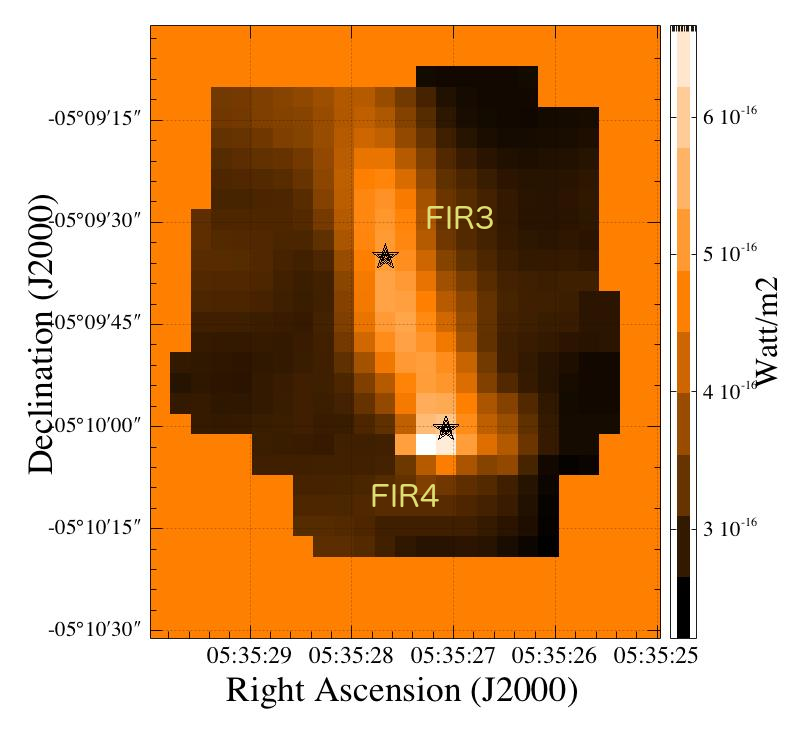
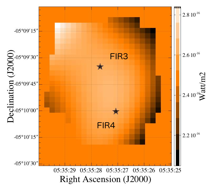
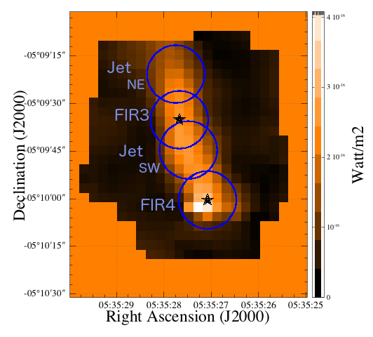
Figure 2: (Top left): [O I] 63 $\mu\mathrm{m}$ line map of the OMC-2 region. (Top right): Extended emission component extracted by fitting a third order polynomial to the line map. (Bottom): Narrow ridge like emission component obtained after subtracting the extended emission background component. Positions, sizes, and names of the line flux aperture measurements listed in Table 2 are indicated.

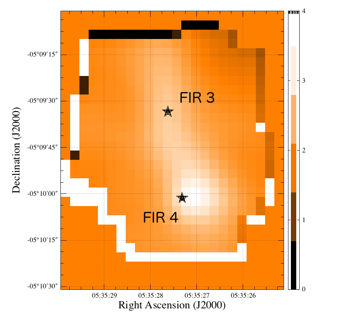
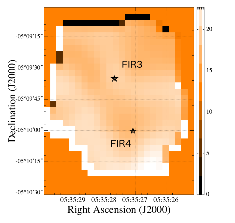
Figure 3: (Left): [O I] 63 $\mu\mathrm{m}$ / [C II] 158 $\mu\mathrm{m}$ map, (Right): [O I] 63 $\mu\mathrm{m}$  / [O I] 145 $\mu\mathrm{m}$ map. All line ratios are calculated at matched angular resolution.

The OMC-2 region in Orion A is one of the richest targets for [O I] studies of outflows from intermediate mass protostars. It contains a group of eight protostars with luminosities of a 20 to 360 $L_{\odot}$ (Adams et al. 2012; Furlan et al. 2016), much higher than the typical luminosity of 1 $L_{\odot}$ for the peak of the protostellar luminosity function of the Orion protostars (Kryukova et al. 2012; Furlan et al. 2016). OMC-2, part of a 2 pc long, dense filament which extends between the Orion Nebula Cluster (ONC) to the south and NGC 1977 to the north, hosts a higher than average fraction of young Class 0 protostars (Chini et al. 1997; Peterson & Megeath 2008; Adams et al. 2012; Megeath et al. 2012; Stutz & Kainulainen 2015).

In this paper, we present data obtained as part of the Herschel Orion Protostar Survey (HOPS) open time key program. We analyze Herschel/ PACS fine structure line observations of the OMC-2 protostars FIR 3 (HOPS 370, VLA 11) and FIR 4 (HOPS 108, VLA 12) (see Reipurth et al. 1999; Adams et al. 2012; Furlan et al. 2016). FIR 3 is the most luminous protostar ($L_{\mathrm{bol}}$$=360$ $L_{\odot}$) in OMC-2 and drives a bipolar outflow with one lobe extending to FIR 4 (Williams et al. 2003; Shimajiri et al. 2008). While previous observations indicated that FIR 4 has a luminosity of 1000 $L_{\odot}$ (Crimier et al. 2009), the bolometric luminosity has now been revised to 38 $L_{\odot}$ (see Furlan et al. 2014, for a detailed discussion). Low-$J$ ($J_{up}\leavevmode\nobreak\ \leq$ 3) CO observations do not show a distinct outflow associated with FIR 4. FIR 3 and FIR 4 have the brightest known far-IR line emission in the cloud outside of the Orion nebula (Manoj et al. 2013). While FIR 3 has a far-IR CO luminosity of $\sim$ 0.06 $L_{\odot}$, FIR 4 has a far-IR CO luminosity of $\sim$ 0.2 $L_{\odot}$ and the brightest [O I] and H₂O emission observed among the HOPS sample (Manoj et al. 2013). Moreover, a clear peak in the far-IR line emission is found at the location of FIR 4 (Manoj et al. 2013; Furlan et al. 2014). While our understanding of the nature of FIR 4 is still incomplete (see Osorio et al., in prep.), the [O I] detailed physical nature of FIR 3 is now coming into sharper focus.

We detect, for the first time, a jet in the far-IR [O I] lines from an intermediate mass protostar FIR 3. The jet line luminosity and implied mass loss rate are a factor of 10 higher than typical values for low-mass class 0 protostars. This jet extends from FIR 3 to FIR 4 and is spatially coincident with CO (6-5) outflow observations, demonstrating a connection between FIR 3 and the bright far-IR line emission at the position of FIR 4. We propose that the bright line emission associated with FIR 4 is produced by the FIR 3 jet.

2 Observations & data reduction

2.1 Herschel PACS

The PACS spectroscopic observations of the OMC-2 region were carried out using the Range Spectroscopy mode to achieve a Nyquist-sampled coverage of the $57-196$ $\mu\mathrm{m}$ wavelength range. The region centered on FIR 3 was observed in the full PACS spatial resolution mapping mode, oversampling the beam by using a 3$\times$3 raster in the blue and 2$\times$2 raster in the red channel with sub-pixel raster line step sizes of 3$\arcsec$ and 4.5$\arcsec$, respectively. The region centered on FIR 4 was observed in the single-pointing mode. We applied the unchopped beam-modulation technique developed for crowded-field spectroscopy. In the unchopped mode, off-positions free of cloud emission within 2^∘ from the target were observed to remove the telescope and sky background. The log of PACS observations of the OMC-2 region is given in Table 1.

The Nyquist sampled wavelength range of $57-71$ $\mu\mathrm{m}$ was observed in the third grating order (B3A), the range $71-98$ $\mu\mathrm{m}$ in the second order (B2B), and the range $102-196$ $\mu\mathrm{m}$ in the first order (R1). The second (B2B) and third (B3A) grating orders are observed with the blue camera, while the first order (R1) spectra has been taken with the red camera simultaneously with one of the blue observations. The broad-range spectral scans were repeated 2 times on each raster position for the mapping observations, and 4 times for the pointed observations in order to achieve at least a 5$\sigma$ detection for the diagnostic lines across the sampled area and to improve spectral sampling provided by the sub-pixel offsets between grating scans.

The HOPS 370 (FIR 3) mapping observation was composed of a sequence of on-target raster and off-target pointed observations which ensures the continuum signal-to-noise achieved per raster position is identical to the signal-to-noise achieved within the single off-position observation. The off-block is subtracted from every raster position of the corresponding mapping observation. In order to shorten the timescale between on- and off-blocks each of the B3A/R1 and B2B/R1 observations have been split up into two identical subgroups resulting 4 on- and off observations pairs in total, on the extra cost of $\sim$ 15 min instrument and spacecraft overheads. For the 3$\times$3 blue rasters $\sim$ 89% of time was spent-on source, while for the 2$\times$2 red rasters $\sim$ 75% of the time was used for on-target observations exhibiting an excellent observing efficiency. The HOPS 108 (FIR 4) pointed observations followed a similar design principle except the choice of wavelength range combinations introduces a slightly improved redundancy and deeper detection limit. The on-source time consists $\sim$ 50% of the total observing time of pointed observations.

FIR 3 was observed in 2011 August over a total of 10.4 hrs (including overheads), and FIR 4 was observed on 2012 February over 2.8 hrs. Table 1 gives the observation list, observing mode parameters, covered wavelength ranges and individual integration times. The Herschel nominal absolute pointing accuracies for the periods comprising the observations of FIR 3 and FIR 4 are 1$\aas@@fstack{\prime\prime}$3 and 0$\aas@@fstack{\prime\prime}$9, respectively (Sánchez-Portal et al. 2014). However, in order to improve the short-term relative pointing accuracy (pointing stability), the attitude data were reprocessed by means of a ground reconstruction procedure making use of the data from the gyroscopes. This procedure improves the instrumental PSF and gives a very uniform absolute pointing accuracy of 1$\aas@@fstack{\prime\prime}$2 across the periods of the mission relevant to this paper. However, the observations of FIR 4 were carried with a solar aspect angle (SAA) of about 102.5^∘. At such angles, some pointing shifts due to structural thermoelastic effects could be expected (Sánchez-Portal et al. 2014) and hence a conservative accuracy figure of [O I] 2$\aas@@fstack{\prime\prime}$0 is advisable for this second target.

The data were reduced with the Herschel interactive processing environment (HIPE v12.1 and calibration v65; Ott (2010)) employing the standard unchopped long-range spectroscopy data processing script to achieve spatially calibrated spectral maps. We applied the standard flux calibration scheme, where the system response applicable to an observation ID is estimated from a calibration block at key wavelengths. The calibration block is executed at the beginning of each on- and off-source observation and the derived system response is adopted for the duration of the observation. The absolute flux level is propagated from the key wavelengths to the covered wavelengths range applying the relative spectral response function (RSRF). Unchopped raw data suffer from instantaneous system response drifts due to cosmic-ray impacts on detectors. Unlike in the case of chop/nod observing mode where drifts are largely eliminated at the chopping frequency in the chop_on-chop_off differential signal, any drifts occurring at timescales shorter than the observation itself remains a property of raw unchopped data. As part of the standard pipeline spectral flat-field task, the continuum sampled by each of the 16 spectral pixels was scaled to the median value to correct for residual flat field effects and to take advantage of redundancy in the data to minimise the impact of eventual drifting pixels. In the final step, flux calibrated cubes are created by subtracting on-off pairs to completely remove the sky and telescope background. On each individual off-subtracted spectral cubes we apply a multi-resolution wavelet based continuum subtraction before data are projected into the final hypersectral cubes. Using this adaptive technique any post-calibration residual continuum wiggles broader than  5-7$\times$ the width of an unresolved line can be efficiently eliminated from the spectra.

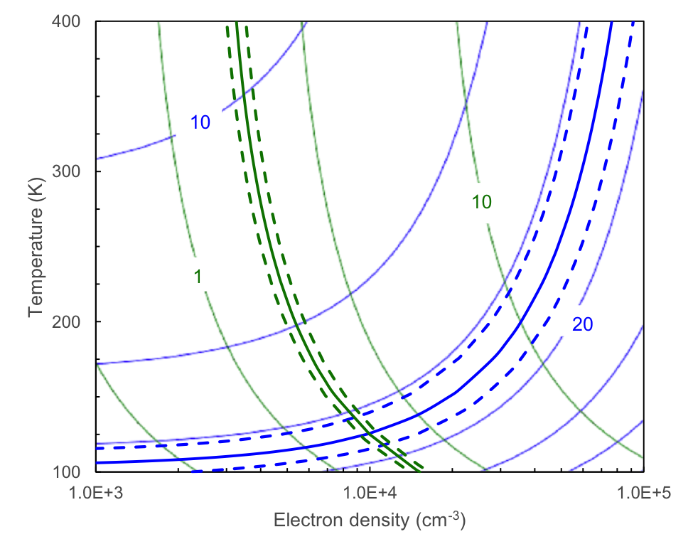
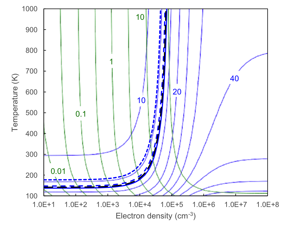
Figure 4: (Top): observed [O I] 63.2/145.5 (blue) and [O I] 63.2/[C II] 157.7 line ratio (green) contours compared to expectations for a single-component model. The observed ratios for the regions immediately outside the FIR 3 jet are indicated with heavy solid contours, and the $\pm$1 $\sigma$ band by dashed contours. Thin contours indicate the constant line ratios, covering the plotted range of density and temperature, with logarithmically-spaced contours. The families of curves intersect near $n_{e}$ = 10⁴ $\textrm{cm}^{-3}$ and T = 130 K, which lie in the ranges common for photodissociation regions in the Orion molecular-cloud complex. (Bottom): [O I] 63.2/145.5 intensity ratios observed along the jet plotted as heavy blue curves: FIR 4 (shortest dashes), FIR 3 (solid), SW/NE of FIR 3 (medium/long dashes). At high temperatures the intensity ratios would indicate electron density in the range 5$\times$10⁴ - 8$\times$10⁴ $\textrm{cm}^{-3}$.

2.2 CO observations

We also obtained CO J=6-5 map of the OMC-2 region made with the CHAMP+ seven element receiver array on the APEX 12 meter telescope. The CO map has 9″ resolution similar to the 63 $\mu$m [O I] map. The details of these observations will be published in a forthcoming paper on a CHAMP survey of several Orion protostars.

3 Analysis and results

The [O I] 63 $\mu\mathrm{m}$ line map of the OMC-2 region is presented in Figure 2. Inspection of the line map reveals a jet: a narrow spatially collimated emission feature connecting FIR 3 and FIR 4. The jet feature is seen superposed on an uniform extended emission. In the following we show that the extended background component is consistent with the emission from a photodissociation region (PDR) on the surface of the OMC-2 cloud.

3.1 Extended PDR emission in OMC-2

The spatial morphology of the fine structure line emission indicates the presence of uniform extended emission in the OMC-2 region. Figure 3 shows the [O I] 63 $\mu\mathrm{m}$ to [CII] and [O I] 63 to 145 $\mu\mathrm{m}$ line ratio maps. The line ratios of the extended emission are approximately constant and distinct from the narrow jet-like emission, indicating a different physical origin for the extended emission. The OMC-2 region lies between the Orion Nebula Cluster (ONC) to the south and NGC 1977 to the north-east, both of which contain OB stars (Peterson & Megeath 2008) and the UV radiation from which can produce photodissociation regions (PDRs) on the surface of molecular clouds.

To quantify the emission from the extended component, we measured the line ratios in six 15″$\times$ 15″regions, three on either side of the jet. The line ratios are remarkably constant between the boxes:
${[\mathrm{O\leavevmode\nobreak\ I}]63}/{[\mathrm{C\leavevmode\nobreak\ II}]158}=1.9\pm 0.1$ ,
${[\mathrm{O\leavevmode\nobreak\ I}]63}/{[\mathrm{O\leavevmode\nobreak\ I}]146}=17\pm 1$.
We compared these line ratios to those expected for a cloud with uniform density and temperature in order to estimate the physical conditions of the extended emission region. If we imagine each [O I] and [C II] line-emission region to have a uniform density and temperature, we can derive useful characteristic densities and temperatures from the line intensity ratios, under the common assumptions that the lines are optically thin and unextinguished, the atomic energy levels are collisionally excited, and the energy-level populations are in steady state (e.g., Osterbrock & Ferland 2006).

Figure 4 contains results of such calculations for the intensity ratios we observe for the FIR 3 jet and for the adjacent cloud emission. We considered only the five lowest-energy levels for neutral oxygen, and the two lowest-energy levels for ionized carbon, to have significant population. We invoked only electrons as collision partners, as these rates dominate those from protons and hydrogen even when the ionization fraction is small. We took the relative abundance of C⁺ and O to be the solar-system C/O ratio, 0.46 (Lodders & Palme 2009). We used the collision strengths computed by Bell et al. (1998) and Zatsarinny & Tayal (2003) for $e-$O, and by Tayal (2008) for $e-$C⁺. Finally, we used the Einstein A-coefficients computed by Froese Fischer & Tachiev (2004) and Wiese & Fuhr (2007) for [O I] and [C II] respectively.

The observed line ratios give an electron density of $n_{e}$$\sim$10⁴ $\textrm{cm}^{-3}$ and T = 130 K for the extended emission component (see Figure 4), appropriate for PDRs with incident FUV field strength of $G_{0}\sim$ 100 (Kaufman et al. 1999). The values for $n_{e}$, T and $G_{0}$ that we obtain lie in the ranges commonly observed for PDRs on the surface of molecular clouds (Hollenbach & Tielens 1997, 1999), indicating that the extended component surrounding the jet is consistent with the emission from a photodissociation region (PDR) on the surface of the OMC-2 cloud.

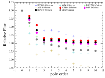
Figure 5: Flux from apertures along the jet for different polynomial order fits relative to zero order fit shown as a function of the polynomial order used for subtracting the extended background emission component.

3.2 Separation of the extended PDR and the jet components

We isolated the jet component from the PDR background for further analysis. We first extracted the extended emission component by fitting the line image with a third order polynomial after masking the central ridge like emission component above 30% of the peak emission detected in the mapped area. We used a third order polynomial to fit the background because it was found to be optimal. Higher order polynomial fits did not improve the background subtraction significantly. This is illustrated in Figure 5, where we show the flux extracted from different apertures on the jet after subtracting the background by fitting polynomials of orders 0 to 10 divided by the flux extracted at the 0 order polynomial. The flux obtained for different polynomial orders are shown relative to that for the zeroth order polynomial fit. For both the [O I] 63 $\mu\mathrm{m}$ and [O I] 145 $\mu\mathrm{m}$  there is no significant improvement beyond a 3^rd polynomial fit to the background emission.

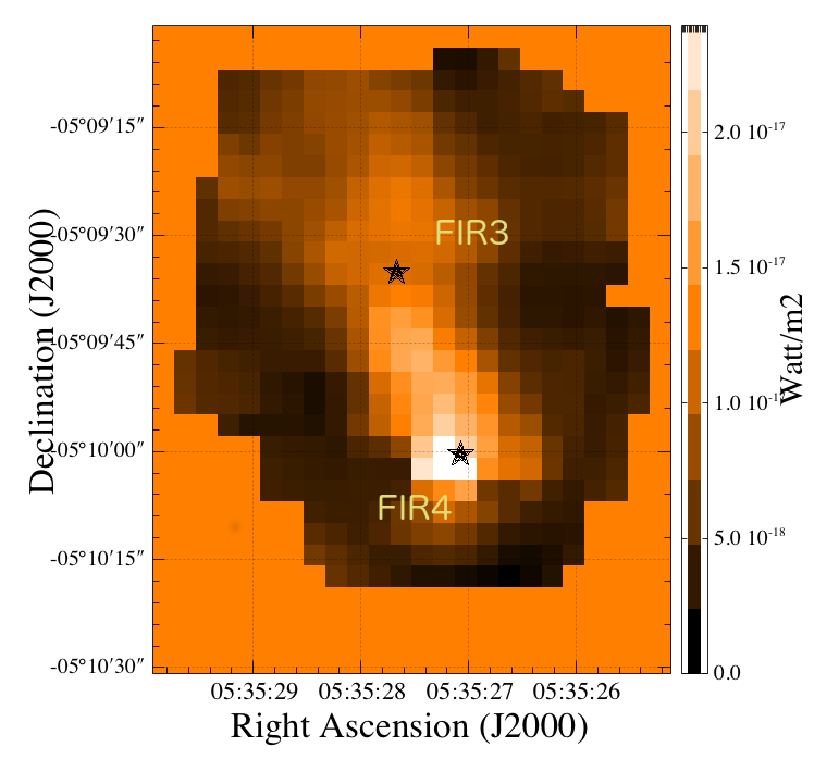
Figure 6: (Left): [O I] 145 $\mu\mathrm{m}$ line map and (Right): [O I] 63 / [O I] 145 line ratio map, both after the subtraction of the extended component.

We then subtracted the extended emission component from the total emission map. Figure 2 shows the total [O I] 63 $\mu\mathrm{m}$ line emission map, the background component and the residual jet component after subtracting the extended background. The procedure was repeated for [O I] 145 $\mu\mathrm{m}$ and the results are shown in Figure 6. Flux values on the jet component have been summed up within 9″synthetic radii apertures. The central locations of the four apertures are indicated on Figure 2 and the line fluxes are listed in Table 2. The statistical uncertainties in the extracted line fluxes were estimated from the fluctuations in the background-subtracted line images measured at several positions located off the jet. These include rms fluctuations due to both the noise in the observed line and the residual from the PDR subtraction. The rms noise of the [O I] 63 $\mu\mathrm{m}$ line map is found to be 2.6 $\times$ 10^-17 Wm^-2 per pixel while that for [O I] 145 $\mu\mathrm{m}$ line map is 3.5 $\times$ 10^-18 Wm^-2 per pixel. Uncertainties corresponding to the line flux integrated over 9″ radius apertures are listed in Table 2.

3.3 The jet morphology

The [O I] jet has a north-east to south-west orientation. The jet emission extends from the edge of the mapped area in the north-east, through FIR 3, and finally terminates at the location of FIR 4 in the south-west, where the [O I] emission is the brightest. Figure 7 shows contours of the [O I] 63 $\mu\mathrm{m}$ jet on a Spitzer/IRAC 4.5 $\mu\mathrm{m}$ image (Megeath et al. 2012). The 4.5 $\mu\mathrm{m}$ band contains bright H₂ emission which traces the shocked molecular gas excited by the jet. We observe a prominent extended 4.5 $\mu\mathrm{m}$ jet terminating in a bow shock to the north-east of FIR-3 (extending past the PACS line map coverage). The 4.5 $\mu\mathrm{m}$ jet emission clearly appears to be driven by FIR 3; however, the counter-jet traced by [O I] is not readily seen at 4.5 $\mu\mathrm{m}$. Figure 7 also shows an overlay of blue- and red-shifted CO (6-5) outflow emission which traces the molecular gas entrained by the jet. The CO emission clearly follows the north-east component of the 4.5 $\mu\mathrm{m}$ jet as well as the [O I] emission extending to the south-west and terminating at FIR 4. Since both CO outflow lobes have high-velocity line wings on both sides of the systemic velocity, the outflow must lie close to the plane of the sky. The combined morphology of all three emission components ([O I], 4.5 $\mu\mathrm{m}$, and CO) strongly suggests that the jet/outflow is driven by FIR 3.

3.4 Excitation conditions in the jet

To investigate the physical conditions along the jet, we measured the [O I] 63 $\mu\mathrm{m}$/145 $\mu\mathrm{m}$ line ratio at four different locations along the jet (Table 2). We compare the observed ratios to predictions for a cloud with uniform density and temperature, described in Section 3.1 and Figure 4. At the high temperatures expected in the dissociative shocks in jets, the line ratio is insensitive to the precise temperature, and indicates electron density ($n_{e}$) in the range of 5-8$\times$10⁴ $\textrm{cm}^{-3}$ (see Figure 4). The $n_{e}$ values for the four different sections of the jet were computed for T = 3000 K (see Table 2). The densities that we derive appear to suggest a gradient along the jet with the density of the jet decreasing with increasing distance from FIR 3. However, the variations in the density along the jet are not significantly above the associated uncertainties, so the presence of a density gradient in the jet cannot be established.

Table 2: Observed properties of the [O I] jet from FIR 3

Position	RA(J2000)	Dec(J2000)	[O I] 63 $\mu\mathrm{m}$		Mass-loss rate	[O I] 63 $\mu\mathrm{m}$/145 $\mu\mathrm{m}$	Electron density
along the jet			Line flux	Line luminosity	$\dot{M}_{out}$	flux ratio	$n_{e}$
			($\times$ 10-15 Wm-2)	($\times$ 10-2 L⊙)	($\times$ 10-6 M⊙yr-1)		($\times$ 104 $\textrm{cm}^{-3}$)
FIR 4	5 35 27.07	$-$5 10 0.37	5.1 $\pm$ 0.14	2.8	2.3	12.2 $\pm$ 0.7	4.8 $\pm$ 0.7
JetSW	5 35 27.48	$-$5 09 44.64	5.2 $\pm$ 0.14	2.8	2.3	13.5 $\pm$ 0.8	6.5 $\pm$ 0.9
FIR 3	5 35 27.67	$-$5 09 35.10	4.8 $\pm$ 0.14	2.6	2.1	14.1 $\pm$ 1.0	7.4 $\pm$ 1.1
JetNE	5 35 27.74	$-$5 09 20.70	3.8 $\pm$ 0.14	2.1	1.7	13.8 $\pm$ 1.2	7.0 $\pm$ 1.4
Entire jet			17.3$\pm$0.3	9.5	7.7

3.5 Mass-loss rates from jets

The [O I] 63 $\mu\mathrm{m}$ line luminosity provides a direct measure of the mass loss rates from protostars (Hollenbach 1985; Hollenbach & McKee 1989). This line is the primary coolant of the predominantly atomic gas in the postshock gas for temperatures in the range of 5000-500 K. The [O I] line luminosity of a planar shocked region is proportional to the rate at which jet material flows into the shock front, or the mass loss rate of the driving source, given by
$\dot{M}_{out}=8.1\times 10^{-5}(L_{[O\leavevmode\nobreak\ I]}/L_{\odot})\leavevmode\nobreak\ \textrm{M${}_{\odot}$\leavevmode\nobreak\ yr${}^{-1}$}$.
Presuming a protostar’s mass loss rate to be constant over the dynamical time of the jet, and neglecting emission from shocks within the jet, the total [O I] 63 $\mu\mathrm{m}$ luminosity, seen from a protostar’s outflow thus yields the protostar’s mass-loss rate. With these caveats, the mass loss rate for FIR3, corresponding to the total [O I] 63 $\mu\mathrm{m}$ luminosity we observe in the jet is 7.7$\times$10^-6 M_⊙ yr^-1. The total [O I] flux was measured from the PDR subtracted line map by adding up all the pixels with flux values $\geq$ 3 $\times$ the rms of the map (Table 2). We also computed the shock flow rates at four different locations along the jet from the [O I] luminosities measured within 9″of the positions listed in Table 2 (also see Figure 2). The flow rates at different sections of the jets lie within a narrow range of 1.7-2.3 $\times$10^-6 M_⊙ yr^-1 and differ only by 26% at most, indicating that the mass flow along the jet is relatively smooth and continuous.

Mass-loss rates from protostars are closely connected to mass accretion rate onto protostars: theoretical models of jet launching predict a proportionality between mass loss rate and mass accretion rate,
$\dot{M}_{out}$ = $b\>\dot{M}_{acc}$,
where $b$ has a theoretical as well as a mean observed value near 0.1 (Pelletier & Pudritz 1992; Watson et al. 2015). The mass flow rate of $\dot{M}_{out}$ = 2.3$\times$10^-6 M_⊙ yr^-1 at the location of FIR 4 implies a mass accretion rate, $\dot{M}_{\mathrm{acc}}$ = 2.3$\times$10^-5 M_⊙ yr^-1, which corresponds to an accretion-luminosity, $L_{\mathrm{acc}}$ = 350 $L_{\odot}$, assuming
$R_{\star}$/$M_{\star}$ = 1 $R_{\odot}$/$M_{\odot}$,
appropriate for intermediate-mass young stars on the birth line (Palla & Stahler 1993). This value of $L_{\mathrm{acc}}$ is close to a factor of 10 higher than the observed $L_{\mathrm{bol}}$ for FIR 4. Further, as noted by Furlan et al. (2014), the true luminosity of FIR 4 could be as small as 14 $L_{\odot}$. On the other hand, the $L_{\mathrm{acc}}$ that we derive is consistent with the observed $L_{\mathrm{bol}}$ for FIR 3. Moreover, the $\dot{M}_{\mathrm{acc}}$ values indicated by the mass loss rates derived from [O I] is remarkably close to the envelope infall rate of 1$\times$10^-5 M_⊙ yr^-1 estimated for FIR 3 from the radiative transfer modeling of the observed broad band spectral energy distribution (Adams et al. 2012; Furlan et al. 2016). All these different lines of argument strongly suggest that the [O I] jet is driven by FIR 3.

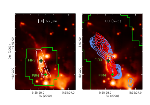
Figure 7: (Left): [O I] 63 $\mu$m line emission (white contours; levels = 1, 2 & 3 $\times$10^-16 Wm^-2/pixel) with the FOV outlined in green. (Right): blue ($-$10 to 9 km s^-1) and red (14 to 30 km s^-1) wings of the CO 6-5 are the blue and red contours. Both are overlaid on the 4.5 $\mu$m image, which shows the jet extending to the north-east.

4 Discussion

Our analysis indicates that the [O I] jet connecting FIR 3 and FIR 4 actually originates from the FIR 3 protostar. Although our Herschel/PACS line maps do not cover the full extent of the north-eastern portion of the 4.5 $\mu\mathrm{m}$ shocked emission, the [O I] jet is observed on either side of FIR 3 and terminates at FIR 4. The jet is also spatially aligned with the CO (6-5) outflow, which extends to FIR 4 in the south. The near constant mass loss rate found along the [O I] jet, indicating a steady and continuous mass flow, also suggests that FIR 3 is driving the jet. The mass flow rate close to FIR 3 and 20″(8400 AU) away at the location of FIR 4 are very similar. It is highly unlikely that FIR 4, which is $\sim$ 10 times less luminous than FIR 3 is driving a jet with mass-flow rate similar to that of FIR 3. These pieces of evidence strongly suggest that the driving source of the observed [O I] jet is FIR 3.

The peak [O I] emission, nevertheless, is observed close to FIR 4. All the high-excitation molecular cooling lines in the far-IR (H₂O, CO and OH) observed with Herschel/PACS also have their peak emission at the location of FIR 4 (Furlan et al. 2014, Manoj et al. in prep). In fact, FIR 4 is one of the brightest far-IR line emitting source among all the protostars observed by HOPS. The far-IR line luminosities measured within a 9.4″aperture around FIR 4 is more than 4$\times$ higher than that observed for FIR 3 (Manoj et al. 2013). Our analysis and other studies of the region, however, do not show any evidence for FIR 4 driving a powerful outflow/jet which could excite such intense line emission. We argue, therefore, that the bright line emission seen toward FIR 4 is the terminal shock (Mach disk) of the FIR 3 jet. Such terminal shocks are often the brightest features of YSO jets, and comprise many of the best-known Herbig-Haro objects. FIR 4 may simply lie along the line of sight and may not even be physically associated with the shocked emitting region.

The jet driven by FIR 3 is the first to be imaged in [O I] 63 $\mu\mathrm{m}$ from an intermediate-mass protostar. [O I] jets from low mass class 0 protostars observed with Herschel/PACS by Nisini et al. (2015) show mass-loss rates in the range of 1-4 $\times$10^-7 M_⊙ yr^-1. These mass-loss rates are more than an order of magnitude lower than that of FIR 3. The mass loss rate for FIR 3 is higher than even the relatively high mass-loss rate of 2-4 $\times$10^-6 M_⊙ yr^-1 found for HH 46 by Nisini et al. (2015). Thus our results indicate that the mass-loss rates in intermediate-mass protostars are $\ga$ 10 times higher than that observed for most low-mass class 0 protostars, consistent with the idea that they drive more powerful jets than their low-mass counterparts.