A generalised multicomponent system of Camassa-Holm-Novikov equations

Abstract

In this paper we introduce a two-component system, depending on a parameter $b$, which generalises the Camassa-Holm ($b=1$) and Novikov equations ($b=2$). By investigating its Lie algebra of classical and higher symmetries up to order $3$, we found that for $b\neq 2$ the system admits a $3$-dimensional algebra of point symmetries and apparently no higher symmetries, whereas for $b=2$ it has a $6$-dimensional algebra of point symmetries and also higher order symmetries. Also we provide all conservation laws, with first order characteristics, which are admitted by the system for $b=1,2$. In addition, for $b=2$, we show that the system is a particular instance of a more general system which admits an $\mathfrak{sl}(3,\mathbb{R})$-valued zero-curvature representation. Finally, we found that the system admits peakon solutions and, in particular, for $b=2$ there exist 1-peakon solutions with non-constant amplitude.

1 Introduction

Since the seminal paper by Camassa and Holm [8], hundreds works have been devoted to several aspects of nonlocal evolution equations of the Camassa-Holm (CH) type, such as: integrability, in the sense of the existence of infinite symmetries [13, 23, 33, 34, 35], existence of bi-hamiltonian formulation and Lax pairs [13, 23, 35, 37], and existence of (multi-) peakon solutions [13, 23]. Further aspects of these classes of equations have also been widely investigated from many different points of view, see [16, 17, 18, 21, 29]. Also, some works considering systems with many components of CH type equations have been of interest, see e.g. [15, 22, 31].

More recently, equations with parameter-dependent nonlinearities have been considered, see for instance [3, 10, 11, 19, 20], where families of equations unifying both Camassa-Holm and Novikov equations [23, 35] are studied.

Motivated by the works [3, 10, 11], in this paper we consider the system

$$\begin{array}[]{l}\left\{\begin{array}[]{l}m_{t}+(b+1)\,u_{x}\,v^{b-1}\,m+u^{b-1}\,v\,m_{x}=0,\\ \\ n_{t}+(b+1)\,v_{x}\,u^{b-1}\,n+v^{b-1}\,u\,n_{x}=0,\end{array}\right.\end{array}$$ (1)

where $u=u(x,t)$, $v=v(x,t)$, $m=u-u_{xx}$ and $n=v-v_{xx}$ are referred to as the momenta and $b\in\mathbb{R}$.

System (1) is invariant under the change $(u,v)\mapsto(v,u)$. In particular, when $u=v$ the system reduces to

$$m_{t}+(b+1)\,u_{x}\,u^{b-1}\,m+u^{b}\,m_{x}=0.$$ (2)

Interestingly, equation (2) reduces to CH equation for $b=1$, and to Novikov equation for $b=2$. Therefore, one may consider system (1) as a two-component generalisation of both CH and Novikov equations. Equation (2) is just the equation deduced in [10], by using symmetry arguments and techniques introduced in [24, 25]. In [11] equation (2) was also re-obtained by imposing invariance under scalings and the existence of a certain multiplier (see [1, 2] for further details). Later, in [3] it was proved that (2) admits peakon and multi-peakon solutions. Other properties of (2) were also investigated by Himonas and Holliman in the paper [18], by embedding it into a two-parameter family of equations.

In this paper we shall investigate system (1) from several points of view. In Section 2 we compute symmetries and conservation laws. In particular, we investigate the existence of higher order, or generalised, symmetries. Then, in Section 3, we show that (1) can be embedded in a $4$-component system admitting an $\mathfrak{sl}(3,\mathbb{R})-$valued zero-curvature representation (ZCR) which generalizes an analog result of paper [32]. In Section 4 we investigate the existence of peakon and multi-peakon solutions of (1). Finally, our results are discussed in Section 5.

2 Symmetries and conservation laws of system $(\ref{1.1})$

In this section we collect the results of the search of classical and higher symmetries of system $(\ref{1.1})$, as well as of low order conservation laws.

2.1 Classical and higher symmetries

By standard methods of symmetry analysis (see e.g. [4, 5, 6, 27, 36, 39]) one can prove the following

Theorem 1

When $b\neq 2$, the Lie algebra of classical symmetries of $(\ref{1.1})$ is $3$-dimensional with generators

$$X_{1}=\frac{\partial}{\partial x},\quad X_{2}=\frac{\partial}{\partial t},\quad X_{3}=bt\frac{\partial}{\partial t}-u\frac{\partial}{\partial u}-v\frac{\partial}{\partial v}.$$ (3)

On the contrary, for $b=2$, Lie algebra of classical symmetries of $(\ref{1.1})$ is $6$-dimensional, with generators $X_{1}$, $X_{2}$, $X_{3}$ (where $b=2$), and

$$X_{4}=u\frac{\partial}{\partial u}-v\frac{\partial}{\partial v},\quad X_{i}=e^{2\epsilon_{i}x}(\frac{\partial}{\partial x}+\epsilon_{i}u\frac{\partial}{\partial u}+\epsilon_{i}v\frac{\partial}{\partial v}),\qquad$$ (4)

with $i=5,6$ and $\epsilon_{5}=1$, $\epsilon_{6}=-1$.

Therefore, by computing the flows of classical symmetries admitted by (1) one gets the following

Corollary 1

Under the flows $\left\{A_{s_{i}}\right\}$ of classical symmetries $X_{i}$, $i=1,2,...,6$, where the $s_{i}$’s denote the flow-parameters, solutions $\left\{u=u(x,t),\,v=v(x,t)\right\}$ of $(\ref{1.1})$ respectively transform to:
$1)\;\left\{u_{1}=u(x-s_{1},t),\,v_{1}=v(x-s_{1},t)\right\}$;
$2)\;\left\{u_{2}=u(x,t-s_{2}),\,v_{1}=v(x,t-s_{2})\right\}$;
$3)\;\left\{u_{3}=e^{s_{3}}u\left(x,te^{-bs_{3}}\right),\,v_{3}=e^{s_{3}}v\left(x,te^{-bs_{3}}\right)\right\}$;
$4)\;\left\{u_{4}=e^{-s_{4}}u\left(x,t\right),\,v_{4}=e^{-s_{4}}v\left(x,t\right)\right\}$;
$5)\;\left\{u_{5}=\sqrt{1+2s_{5}e^{2x}}u\left(-\frac{1}{2}\ln\left(2s_{5}+e^{-2x}\right),t\right),\,v_{5}=\sqrt{1+2s_{5}e^{2x}}v\left(-\frac{1}{2}\ln\left(2s_{5}+e^{-2x}\right),t\right)\right\}$;
$6)\;\left\{u_{6}=\sqrt{1-2s_{6}e^{-2x}}u\left(\frac{1}{2}\ln\left(-2s_{6}+e^{2x}\right),t\right),\,v_{6}=\sqrt{1-2s_{6}e^{-2x}}v\left(\frac{1}{2}\ln\left(-2s_{6}+e^{2x}\right),t\right)\right\}$.

The special character suggested by Theorem 1 for the case $b=2$ is further confirmed by the search of higher order (or generalised) symmetries. Indeed, we have not found any higher order symmetry for $b\neq 2$, whereas for $b=2$ we found the following

Theorem 2

When $b=2$ system $(\ref{1.1})$ admits higher order symmetries. Moreover, up to order $3$, higher symmetries in evolutionary form

$$Y=\sum_{|\sigma|\geq 0}D_{\sigma}(\phi)\frac{\partial}{\partial u_{\sigma}}+\sum_{|\sigma|\geq 0}D_{\sigma}(\psi)\frac{\partial}{\partial v_{\sigma}}$$

are described by the characteristics (or generating functions) $Q=(\phi,\psi)$:

$$\phi={\displaystyle\sum_{i=1}^{9}}c_{i}\phi_{i}\qquad\psi={\displaystyle\sum_{i=1}^{9}}c_{i}\psi_{i}$$

where $Q_{i}=(\phi_{i},\psi_{i})$, for $i=1,...,6$, are the characteristics of classical symmetries $X_{i}$ (see Theorem 1), whereas for $i=7,8,9$ are given by

$$\phi_{7}=\frac{\left(u-u_{xx}\right)^{1/3}}{\left(v-v_{xx}\right)^{2/3}},\qquad\psi_{7}=\frac{\left(-v+v_{xx}\right)^{1/3}}{\left(u-u_{xx}\right)^{2/3}},$$

$$\begin{array}[]{l}\phi_{8}=2\left(vv_{xx}+v_{x}^{2}-\frac{3}{2}v^{2}\right)u^{3}+2u\left(v^{2}u_{x}^{2}-u_{x}v_{t}\right)-u_{tt}\vspace{10pt}\\ \qquad+4u^{2}\left(\frac{1}{4}v^{2}u_{xx}-vv_{x}u_{x}+\frac{1}{2}v_{xt}\right),\vspace{10pt}\\ \psi_{8}=-2\left(u_{x}^{2}+uu_{xx}-\frac{3}{2}u^{2}\right)v^{3}+2v\left(-v_{x}^{2}u^{2}+u_{t}v_{x}\right)+v_{tt}\vspace{10pt}\\ \qquad+4v^{2}\left(-\frac{1}{4}u^{2}v_{xx}+uv_{x}u_{x}-\frac{1}{2}u_{xt}\right),\end{array}$$

$$\begin{array}[]{l}\phi_{9}={\displaystyle\frac{1}{2}}\left({\displaystyle v^{2}u{\it u_{t}}}-{\displaystyle v^{3}u^{2}u_{x}}\right){\it u_{xx}}+{\displaystyle\frac{1}{2}}\left(-u^{2}vv_{x}+uv^{2}u_{x}-uv_{t}\right){\it u_{tx}\vspace{10pt}}\\ \qquad+\left({\displaystyle\frac{v^{2}u_{x}^{2}}{2}}-{\displaystyle\frac{1}{2}}\left({\it v_{t}}+3uvv_{x}\right)u_{x}+u^{2}v_{x}^{2}+u^{2}vv_{xx}+uv_{tx}-{\displaystyle\frac{3}{2}}v^{2}u^{2}\right)u_{t}\vspace{10pt}\\ \qquad-{\displaystyle\frac{1}{6}}u^{3}v^{3}u_{xxx}+{\displaystyle\frac{2}{3}}u^{3}v^{3}u_{x}-{\displaystyle\frac{1}{6}}u_{ttt},\vspace{10pt}\\ \psi_{9}={\displaystyle\frac{1}{2}}\left({\displaystyle u^{2}v{\it v_{t}}}-{\displaystyle u^{3}v^{2}v_{x}}\right){\it v_{xx}}+{\displaystyle\frac{1}{2}}\left(-v^{2}uu_{x}+vu^{2}v_{x}-vu_{t}\right){\it v_{tx}}\vspace{10pt},\\ \qquad+\left({\displaystyle\frac{u^{2}v_{x}^{2}}{2}}-{\displaystyle\frac{1}{2}}\left({\it u_{t}}+3vuu_{x}\right)v_{x}+v^{2}u_{x}^{2}+v^{2}uu_{xx}+vu_{tx}-{\displaystyle\frac{3}{2}}u^{2}v^{2}\right)v_{t}\vspace{10pt}\\ \qquad-{\displaystyle\frac{1}{6}}v^{3}u^{3}v_{xxx}+{\displaystyle\frac{2}{3}}v^{3}u^{3}v_{x}-{\displaystyle\frac{1}{6}}v_{ttt}.\end{array}$$

In particular, the corresponding Lie algebra structure is given by the non trivial Jacobi brackets

$$\begin{array}[]{l}\{Q_{1},Q_{5}\}=2Q_{5},\quad\{Q_{1},Q_{6}\}=-2Q_{6},\quad\{Q_{2},Q_{3}\}=2Q_{2},\vspace{10pt}\\ \{Q_{3},Q_{8}\}=-4Q_{8},\quad\{Q_{3},Q_{9}\}=-6Q_{9},\quad\{Q_{5},Q_{6}\}=-4Q_{1}.\end{array}$$

Theorem 2 provides important indications about the property of system (1) being symmetry-integrable when $b=2$. Indeed, according to the terminology introduced in [28] (see also [14]), Theorem 2 proves that system 1 is almost symmetry-integrable of depth at least $3$. On the contrary, our computations up to order $3$ did not provide any higher symmetry of (1) for $b\neq 2$. Thus, we conjecture that system $(\ref{1.1})$ is symmetry-integrable only in the case $b=2$.

2.2 Conservation laws

We recall that a 1-form $\Lambda=Pdx+Qdt$ is a local conservation law for (1), provided that $d\Lambda\equiv 0$ on the solutions of (1). Local conservation laws form a real vector space and we refer the reader to [1, 2, 39] for the general theory and more details on computation techniques.

In order to find local conservation laws of system (1), one has to satisfy the following condition

$$\begin{array}[]{l}D_{t}(P)-D_{x}(Q)-\varphi\left[m_{t}+(b+1)\,u_{x}\,v^{b-1}\,m+u^{b-1}\,v\,m_{x}\right]\\ \\ -\psi\left[n_{t}+(b+1)\,v_{x}\,u^{b-1}\,n+v^{b-1}\,u\,n_{x}\right]=0,\end{array}$$

where $(\varphi,\psi)$ are the characteristics of the corresponding conservation laws.

By performing all needed computations, for cases $b=1$ and $b=2$ with first order characteristics, we find the following

Theorem 3

The space of nontrivial conservation laws with first order characteristics of system $(\ref{1.1})$ is $1$-dimensional for $b=1$ and $5$-dimensional for $b=2$, with generators $\Lambda=Pdx+Qdt$ given in Table 1.

Table 1: Low order conservation laws for system (1) with $b=1$ and $b=2$.

			Components of conserved vectors
$b$	$\varphi$	$\psi$	$P$ (density)	$Q$ (flux)
1	1	1	$u+v$	$\begin{array}[]{l}-v^{2}+v_{x}^{2}-u^{2}+u_{x}^{2}+uv_{xx}\\ -uv+vu_{xx}-v_{x}u_{x}+u_{tx}+v_{tx}\end{array}$
2	$v$	$u$	$uv+u_{x}v_{x}$	$\begin{array}[]{l}(vv_{xx}+v_{x}^{2}-2v^{2})u^{2}+\\ (v_{tx}+v^{2}u_{xx}-2vu_{x}v_{x})u\\ +vu_{tx}+v^{2}u_{x}^{2}\end{array}$
2	$-v_{x}$	$u_{x}$	$(u_{xx}-u)v_{x}$	$\begin{array}[]{l}-v_{x}vu_{x}^{2}+u_{x}v_{tx}\\ +(vu_{x}v_{xx}+u_{x}v_{x}^{2}-u_{xx}vv_{x}-v_{t})u\end{array}$
2	$-v_{t}$	$u_{t}$	$\begin{array}[]{l}((vv_{xx}+v_{x}^{2})uu_{x}\\ +v_{tx}u_{x}+2v_{x}u^{2}v\\ +u_{xx}v_{t}\end{array}$	$\begin{array}[]{l}u_{t}uv_{x}^{2}+2v_{t}vu^{2}-v_{t}vu_{x}^{2}\\ +(vu_{x}u+u_{t})v_{tx}+u_{t}uvv_{xx}\\ +v_{t}(u_{x}v_{x}-u_{xx}v)u+u_{x}v_{tt}\end{array}$
2	$-(v_{x}-v)e^{2x}$	$(u_{x}-u)e^{2x}$	$\begin{array}[]{l}\left[(v_{x}-v)(u_{x}+u_{xx})\right.\\ \left.+u(-v+v_{xx})\right]e^{2x}\end{array}$	$\begin{array}[]{l}\left\{v(v-v_{x})u_{x}^{2}+\left[(v_{xx}v+v_{x}^{2}-2v^{2})u\right.\right.\\ \left.\left.+(v_{tx}-v_{t})\right]u_{x}+v(v-v_{x})uu_{xx}\right.\\ \left.-(v_{x}^{2}+v_{xx}v-2vv_{x})u^{2}+u_{t}(v_{x}-v)\right\}\,\rme^{2x}\end{array}$
2	$-(v_{x}+v)e^{-2x}$	$(u_{x}+u)e^{-2x}$	$\begin{array}[]{l}\left[(2v-v_{x})u_{x}-uv\right.\\ \left.-(u-u_{xx})v_{x}\right]e^{-2x}\end{array}$	$\begin{array}[]{l}\left\{\left[uv_{x}^{2}+(v_{tx}+vv_{xx}u-2v^{2}u)\right]u_{x}\right.\\ -(v^{2}+vv_{x})u_{x}^{2}+u^{2}v_{x}^{2}\\ +uv(2u-u_{xx})v_{x}+(-vu_{tx}+uv_{tx}\\ \left.-u_{xx}v^{2}u+vv_{xx}u^{2}+v_{t}u)\right\}\rme^{-2x}\end{array}$

3 Embedding of (1) with $b=2$ into a new $4$-component system admitting an $\mathfrak{sl}(3,\mathbb{R})-$valued ZCR

In this section we will consider the system (1) with $b=2$, and rewrite it in the form

$$\begin{array}[]{l}\left\{\begin{array}[]{l}D_{t}m_{1}+D_{x}\left(u_{1}\,u_{2}\,m_{1}\right)+\left(-u_{1}\,u_{2x}+2u_{2}u_{1x}\right)m_{1}=0,\\ \\ D_{t}m_{2}+D_{x}\left(u_{1}\,u_{2}\,m_{2}\right)+\left(-u_{2}\,u_{1x}+2u_{1}u_{2x}\right)m_{2}=0,\\ \end{array}\right.\end{array}$$ (5)

where $u_{1}=u$, $u_{2}=v$ and $m_{1}=m$, $m_{2}=n$.

In the paper [15] the authors already considered this system and they found that it admits a zero-curvature representation (ZCR) which depends on a parameter $\lambda$, $\lambda\in\mathbb{R}\setminus\{0\}$. Their ZCR is not $\mathfrak{sl}(3,\mathbb{R})-$valued, nevertheless one can slightly modify their result and check that (5) also admits the $\mathfrak{sl}(3,\mathbb{R})-$valued ZCR $D_{t}X-D_{x}T+\left[X,T\right]=0$, with

$$X=\left(\begin{array}[]{ccc}0&\lambda m_{1}&1\\ 0&0&\lambda m_{2}\\ 1&0&0\end{array}\right),$$

and

$$T=\left(\begin{array}[]{ccc}\frac{1}{3\lambda^{2}}-u_{2}u_{1x}\vspace{10pt}&\frac{u_{1x}}{\lambda}-\lambda u_{1}u_{2}m_{1}\vspace{10pt}&u_{1x}u_{2x}\vspace{10pt}\\ \frac{u_{2}}{\lambda}\vspace{10pt}&-\frac{2}{3\lambda^{2}}+u_{2}u_{1x}-u_{1}u_{2x}\vspace{10pt}&-\lambda u_{1}u_{2}m_{2}+\frac{-u_{2x}}{\lambda}\vspace{10pt}\\ -u_{2}u_{1}&\frac{u_{1}}{\lambda}&\frac{1}{3\lambda^{2}}+u_{1}u_{2x}\end{array}\right).$$

Moreover, in the paper [32] has also been shown that (5) can be embedded in the following $4$-component Camassa-Holm type hierarchy

$$\left\{\begin{array}[]{l}D_{t}m_{1}+D_{x}\left(\Gamma m_{1}\right)-\Gamma n_{2}+g_{1}g_{2}n_{2}+\left(f_{2}g_{2}+2f_{1}g_{1}\right)m_{1}=0,\vspace{5pt}\\ D_{t}m_{2}+D_{x}\left(\Gamma m_{2}\right)+\Gamma n_{1}-g_{1}g_{2}n_{1}-\left(f_{1}g_{1}+2f_{2}g_{2}\right)m_{2}=0,\vspace{5pt}\\ D_{t}n_{1}+D_{x}\left(\Gamma n_{1}\right)+\Gamma m_{2}-f_{1}f_{2}m_{2}-\left(f_{2}g_{2}+2f_{1}g_{1}\right)n_{1}=0,\vspace{5pt}\\ D_{t}n_{2}+D_{x}\left(\Gamma n_{2}\right)-\Gamma m_{1}+f_{1}f_{2}m_{1}+\left(f_{1}g_{1}+2f_{2}g_{2}\right)n_{2}=0,\vspace{5pt}\end{array}\right.$$ (6)

where $m_{i}=u_{i}-u_{ixx}$, $n_{i}=v_{i}-v_{ixx}$, $i=1,2$, $f_{1}=u_{2}-v_{1x}$, $f_{2}=u_{1}+v_{2x}$, $g_{1}=v_{2}+u_{1x}$, $g_{2}=v_{1}-u_{2x}$ and $\Gamma$ is an arbitrary differentiable function of $u_{i},v_{i}$ and their partial derivatives with respect to $x$. As shown in [32], system (6) generalises several well known Camassa-Holm type equations and admits a ZCR too.

Like for [15], also the ZCR originally considered in [32] for the system (6) is not $\mathfrak{sl}(3,\mathbb{R})$-valued. However, one can check that an $\mathfrak{sl}(3,\mathbb{R})-$valued ZCR for (6) is provided by

$$X=\left(\begin{array}[]{ccc}0&\lambda m_{1}&1\\ \lambda n_{1}&0&\lambda m_{2}\\ 1&\lambda n_{2}&0\end{array}\right),$$

$$T=\left(\begin{array}[]{ccc}\frac{1}{3\lambda^{2}}-f_{1}g_{1}\vspace{10pt}&\frac{g_{1}}{\lambda}-\lambda\Gamma m_{1}\vspace{10pt}&-g_{1}g_{2}\vspace{10pt}\\ -\lambda\Gamma n_{1}+\frac{f_{1}}{\lambda}\vspace{10pt}&-\frac{2}{3\lambda^{2}}+f_{1}g_{1}+f_{2}g_{2}\vspace{10pt}&-\lambda\Gamma m_{2}+\frac{g_{2}}{\lambda}\vspace{10pt}\\ -f_{1}f_{2}&-\lambda\Gamma n_{2}+\frac{f_{2}}{\lambda}&\frac{1}{3\lambda^{2}}-f_{2}g_{2}\end{array}\right),$$

where $\lambda\in\mathbb{R}\setminus\{0\}$.

The following result, which follows by direct computations, provides a generalisation of (6) and hence a further generalisation of (5).

Theorem 4

The four-component system

$$\left\{\begin{array}[]{l}D_{t}m_{1}+D_{x}\left(\Gamma m_{1}\right)-\Gamma n_{2}+c_{1}\left(g_{1}g_{2}n_{2}+f_{2}g_{2}m_{1}+2f_{1}g_{1}m_{1}\right)\\ \\ \qquad-3c_{2}m_{1}-c_{3}n_{2}=0,\\ \\ D_{t}m_{2}+D_{x}\left(\Gamma m_{2}\right)+\Gamma n_{1}+c_{1}\left(-g_{1}g_{2}n_{1}-f_{1}g_{1}m_{2}-2f_{2}g_{2}m_{2}\right)\\ \\ \qquad+3c_{2}m_{2}+c_{3}n_{1}=0,\\ \\ D_{t}n_{1}+D_{x}\left(\Gamma n_{1}\right)+\Gamma m_{2}+c_{1}\left(-f_{1}f_{2}m_{2}-f_{2}g_{2}n_{1}-2f_{1}g_{1}n_{1}\right)\\ \\ \qquad+3c_{2}n_{1}+c_{3}m_{2}=0,\\ \\ D_{t}n_{2}+D_{x}\left(\Gamma n_{2}\right)-\Gamma m_{1}+c_{1}\left(f_{1}f_{2}m_{1}+f_{1}g_{1}n_{2}+2f_{2}g_{2}n_{2}\right)\\ \\ \qquad-3c_{2}n_{2}-c_{3}m_{1}=0,\end{array}\right.$$ (7)

where $m_{i}$, $n_{i}$, $f_{i}$, $g_{i}$ are given by

$$\begin{array}[]{l}m_{i}=u_{i}-u_{ixx},\qquad n_{i}=v_{i}-v_{ixx},\quad i=1,2,\vspace{5pt}\\ \\ f_{1}=u_{2}-v_{1x},\quad f_{2}=u_{1}+v_{2x},\quad g_{1}=v_{2}+u_{1x},\quad g_{2}=v_{1}-u_{2x},\end{array}$$

$c_{1},c_{2},c_{3}\in\mathbb{R}$ and $\Gamma$ is an arbitrary differentiable function of $u_{i},v_{i}$ and their derivatives with respect to $x$, admits the zero-curvature representation $D_{t}X-D_{x}T+\left[X,T\right]=0$ defined, for any $\lambda\in\mathbb{R}\setminus\{0\}$, by

$$X=\left(\begin{array}[]{ccc}0&\lambda m_{1}&1\\ \lambda n_{1}&0&\lambda m_{2}\\ 1&\lambda n_{2}&0\end{array}\right)$$

and

$$T=\left(\begin{array}[]{ccc}c_{1}\left(\frac{1}{3\lambda^{2}}-g_{1}f_{1}\right)+c_{2}\vspace{10pt}&c_{1}\frac{g_{1}}{\lambda}-\lambda m_{1}\Gamma\vspace{10pt}&-c_{1}g_{1}g_{2}+c_{3}\vspace{10pt}\\ -\lambda n_{1}\Gamma+c_{1}\frac{f_{1}}{\lambda}\vspace{10pt}&c_{1}\left(-\frac{2}{3\lambda^{2}}+g_{1}f_{1}+g_{2}f_{2}\right)-2c_{2}\vspace{10pt}&-\lambda m_{2}\Gamma+c_{1}\frac{g_{2}}{\lambda}\vspace{10pt}\\ c_{3}-c_{1}f_{1}f_{2}&-\lambda n_{2}\Gamma+c_{1}\frac{f_{2}}{\lambda}&c_{1}\left(\frac{1}{3\lambda^{2}}-g_{2}f_{2}\right)+c_{2}\end{array}\right).$$

System (6) is a particular instance of (7), and in general they are not contact equivalent. In the particular case of (5) this fact readily follows from the following

Theorem 5

By choosing $v_{1}=v_{2}=0$ and $\Gamma=u_{1}u_{2}$, system $(\ref{eq_gen})$ reduces to the system

$$\begin{array}[]{l}\left\{\begin{array}[]{l}D_{t}m_{1}+D_{x}\left(u_{1}\,u_{2}\,m_{1}\right)+c_{1}\left(-u_{1}\,u_{2x}+2u_{2}u_{1x}\right)m_{1}-3c_{2}m_{1}=0,\\ \\ D_{t}m_{2}+D_{x}\left(u_{1}\,u_{2}\,m_{2}\right)+c_{1}\left(-u_{2}\,u_{1x}+2u_{1}u_{2x}\right)m_{2}+3c_{2}m_{2}=0,\\ \end{array}\right.\end{array}$$ (8)

which is not contact equivalent to $(\ref{1.2*})$. In particular, $(\ref{1.3})$ reduces to $(\ref{1.2*})$ when $c_{1}=1,\,c_{2}=0$.

Proof: The structure of the Lie algebra of classical symmetries of (8) depends on $c_{1}$ and $c_{2}$. Indeed, by a direct computation one gets that the dimension of this Lie algebra is $4$ when $c_{1}\neq 1$, and $6$ when $c_{1}=1$. In particular, when $c_{1}\neq 1$ the Lie algebra is described by the characteristics $S_{i}=(\phi_{i},\psi_{i})$, with

$$\phi_{1}=u_{x},\qquad\phi_{2}=u_{t},\qquad\phi_{3}=t\left(3c_{2}u-u_{t}\right),\qquad\phi_{4}=u,$$

and

$$\psi_{1}=v_{x},\qquad\psi_{2}=v_{t},\qquad\psi_{3}=\left(-3c_{2}tv-tv_{t}-v\right),\qquad\psi_{4}=-v.$$

In this first case the only non trivial Jacobi bracket is

$$\begin{array}[]{l}\{S_{2},S_{3}\}=-3c_{2}S_{4}+S_{2}.\end{array}$$

On the contrary, when $c_{1}=1$ the Lie algebra is described by the previous characteristics $S_{i}=(\phi_{i},\psi_{i})$ for $i=1,2,3,4$, and by two further characteristics $S_{5}=(\phi_{5},\psi_{5})$ and $S_{6}=(\phi_{6},\psi_{6})$ given by

$$\phi_{5}=\rme^{-2x}\left(u+u_{x}\right),\qquad\phi_{6}=\rme^{2x}\left(-u+u_{x}\right),$$

and

$$\psi_{5}=\rme^{-2x}\left(v+v_{x}\right),\qquad\psi_{6}=\rme^{2x}\left(-v+v_{x}\right).$$

In this second case the only non trivial Jacobi brackets are

$$\begin{array}[]{l}\{S_{2},S_{3}\}=-3c_{2}S_{4}+S_{2},\qquad\{S_{1},S_{5}\}=2S_{5},\qquad\{S_{1},S_{6}\}=-2S_{6},\qquad\{S_{5},S_{6}\}=-4S_{1}.\end{array}$$

Thus the result follows by the invariance of symmetry algebras under contact transformations. $\square$

4 Multi-peakons

From now on, we assume that $b$ is a positive integer, and make the änsatz that system (1) admits a superposition of peakon solutions of the form

$$u(x,t)=\sum_{i=1}^{N}p_{i}\rme^{-|x-q_{i}|},\quad\quad v(x,t)=\sum_{i=1}^{M}P_{i}\rme^{-|x-Q_{i}|},$$ (9)

where $N$ and $M$ are arbitrary positive integer numbers and $p_{i},\,P_{i},\,q_{i}$ and $Q_{i}$ are $2(N+M)$ smooth functions of $t$. We omitted the explicit dependence on $t$ for sake of simplicity. We shall denote derivative with respect to $t$ as $p^{\prime}_{i},\,P^{\prime}_{i},\,q^{\prime}_{i}$ and $Q^{\prime}_{i}$.

In the distributional sense, see [38] for further details, we have the following results:

$$\begin{array}[]{l}\displaystyle{u_{x}=-\sum_{i=1}^{N}{\rm sign\,}{(x-q_{i})p_{i}}\rme^{-|x-q_{i}|},\,\,v_{x}=-\sum_{i=1}^{M}{\rm sign\,}{(x-Q_{i})P_{i}}\rme^{-|x-Q_{i}|}},\\ \\ \displaystyle{u_{xx}=u-2\sum_{i=1}^{N}p_{i}\delta(x-q_{i}),\quad v_{xx}=v-2\sum_{i=1}^{M}P_{i}\delta(x-Q_{i})}.\end{array}$$ (10)

Thus, one can write the momenta and their derivatives as

$$\begin{array}[]{l}\displaystyle{m=2\sum_{i=1}^{N}p_{i}\delta(x-q_{i}),\,\,n=2\sum_{i=1}^{M}P_{i}\delta(x-Q_{i}),\,\,m_{x}=2\sum_{i=1}^{N}p_{i}\delta^{\prime}(x-q_{i})},\\ \\ \displaystyle{n_{x}=2\sum_{i=1}^{M}P_{i}\delta^{\prime}(x-Q_{i}),\,\,m_{t}=2\sum_{i=1}^{N}\left[p_{i}^{\prime}\delta(x-q_{i})-p_{i}q_{i}^{\prime}\delta^{\prime}(x-q_{i})\right]},\\ \\ \displaystyle{n_{t}=2\sum_{i=1}^{N}\left[P_{i}^{\prime}\delta(x-Q_{i}(t))-P_{i}Q_{i}^{\prime}\delta^{\prime}(x-Q_{i})\right].}\end{array}$$ (11)

Hence, by substituting (9), (10) and (11) into (1), integrating against all pair of test functions with compact support and making use of the regularisation ${\rm sign\,}{(0)}=0$, one gets that the functions $p_{i},\,P_{i},\,q_{i}$ and $Q_{i}$ evolve according to the system of ODEs

$$\begin{array}[]{lcl}\displaystyle{q_{k}^{\prime}}&=&\displaystyle{\left(\sum\limits_{m=1}^{N}p_{m}e^{-|q_{k}-q_{m}|}\right)^{b-1}}\sum\limits_{j=1}^{M}P_{j}e^{-|q_{k}-Q_{j}|},\quad 1\leq k\leq N,\\ \\ \displaystyle{Q_{\sigma}^{\prime}}&=&\displaystyle{\left(\sum\limits_{m=1}^{M}P_{m}\rme^{-|Q_{\sigma}-Q_{m}|}\right)^{b-1}}\sum\limits_{j=1}^{N}p_{j}\rme^{-|Q_{\sigma}-q_{j}|},\quad 1\leq\sigma\leq M,\\ \\ \displaystyle{p_{k}^{\prime}}&=&\displaystyle{p_{k}\left[(b+1)\sum\limits_{j=1}^{N}{\rm sign\,}{(q_{k}-q_{j})p_{j}\rme^{-|q_{k}-q_{j}|}}\left(\sum\limits_{m=1}^{M}P_{m}\rme^{-|q_{k}-Q_{m}|}\right)^{b-1}\right.}\\ \\ &&\displaystyle{\left.-(b-1)\sum\limits_{j=1}^{N}\sum\limits_{l=1}^{M}{\rm sign\,}{(q_{k}-q_{j})}p_{j}P_{l}\rme^{-|q_{k}-q_{j}|-|q_{k}-Q_{l}|}\left(\sum\limits_{m=1}^{N}p_{m}\rme^{-|q_{k}-q_{m}|}\right)^{b-2}\right.}\\ \\ &&\displaystyle{-\left.\sum\limits_{l=1}^{M}{\rm sign\,}{(q_{k}-Q_{l})P_{l}\,\rme^{-|q_{k}-Q_{l}|}}\left(\sum\limits_{m=1}^{N}p_{m}\rme^{-|q_{k}-q_{m}|}\right)^{b-1}\right]},\quad 1\leq k\leq N,\\ \\ \displaystyle{P_{\sigma}^{\prime}}&=&\displaystyle{P_{\sigma}\left[(b+1)\sum\limits_{j=1}^{M}{\rm sign\,}{(Q_{\sigma}-Q_{j})P_{j}\rme^{-|Q_{\sigma}-q_{j}|}}\left(\sum\limits_{m=1}^{N}p_{m}\rme^{-|Q_{\sigma}-q_{m}|}\right)^{b-1}\right.}\\ \\ &&\displaystyle{\left.-(b-1)\sum\limits_{j=1}^{M}\sum\limits_{l=1}^{N}{\rm sign\,}{(Q_{\sigma}-Q_{j})}P_{j}p_{l}\,\rme^{-|Q_{\sigma}-Q_{j}|-|Q_{\sigma}-q_{l}|}\left(\sum\limits_{m=1}^{M}P_{m}\rme^{-|Q_{\sigma}-Q_{m}|}\right)^{b-2}\right.}\\ \\ &&\displaystyle{-\left.\sum\limits_{l=1}^{N}{\rm sign\,}{(Q_{\sigma}-q_{l})p_{l}\,\rme^{-|Q_{\sigma}-q_{l}|}}\left(\sum\limits_{m=1}^{M}P_{m}\,\rme^{-|Q_{\sigma}-Q_{m}|}\right)^{b-1}\right]},\quad 1\leq\sigma\leq M.\end{array}$$ (12)

Obtaining a solution of the system (12) is in general a difficult task, however in the particular case when $N=M$, $q_{j}=Q_{j}$ and $p_{j}=P_{j}$, system (12) reduces to

$$\begin{array}[]{lcl}\displaystyle{q^{\prime}_{k}}&=&\displaystyle{\left(\sum\limits_{j=1}^{N}p_{j}\rme^{-|q_{k}-q_{j}|}\right)^{b}},\\ \\ \displaystyle{p^{\prime}_{k}}&=&\displaystyle{p_{k}\sum\limits_{j=1}^{N}{\rm sign\,}{(q_{k}-q_{j})p_{j}\rme^{-|q_{k}-q_{j}|}}\left(\sum\limits_{j=1}^{N}p_{j}\rme^{-|q_{k}-q_{j}|}\right)^{b-1}},\end{array}$$ (13)

which is a result analogous to that obtained in [3].

Although system (13) shows the consistency of our results with those previously known, it also reflects a noteworthy difference between the scalar case considered in [3] and the two component case of (1). A particularly interesting manifestation of such differences is provided by the properties of $1$-peakon solutions of system (1) which are discussed below.

When $N=M=1$, after rearranging notations, system (12) reads

$$\begin{array}[]{l}q^{\prime}=p^{b-1}P\,\rme^{-|q-Q|},\quad Q^{\prime}=P^{b-1}p\,\rme^{-|Q-q|},\\ \\ p^{\prime}=-{\rm sign\,}{(q-Q)}\,\rme^{-|q-Q|}\,p^{b}P,\quad P^{\prime}={\rm sign\,}{(q-Q)}\,\rme^{-|q-Q|}\,P^{b}p.\end{array}$$ (14)

Thus, in view of (14), one has the following results.

Theorem 6

Assume that $p,\,P,\,q$ and $Q$ are smooth functions satisfying $(\ref{4.7})$, then

$$(q-Q)^{\prime}=pP(p^{b-2}-P^{b-2})\,\rme^{-|q-Q|}$$ (15)

and

$$(p\pm P)^{\prime}=-{\rm sign\,}{(q-Q)}\,\rme^{-|q-Q|}\,pP(p^{b-1}\mp P^{b-1}).$$ (16)

Proof: It follows from (14) by a direct computation.$\square$

Theorem 7

Assume that $p,\,P,\,q$ and $Q$ are smooth functions satisfying $(\ref{4.7})$, and assume that ${\rm sign\,}{(q-Q)}\neq 0$, then

$$\left\{\begin{array}[]{lcl}pP=\kappa,&\quad if&b=2,\\ \\ \displaystyle{\frac{1}{p^{b-2}}+\frac{1}{P^{b-2}}=\kappa,}&\quad if&b\neq 2,\end{array}\right.$$ (17)

where $\kappa$ is a constant.

Proof: It is enough to observe that $p^{\prime}P^{b-1}=-p^{b-1}P^{\prime}$. $\square$

Theorem 8

Assume that $p,\,P,\,q$ and $Q$ are smooth functions satisfying $(\ref{4.7})$, with $b\in\mathbb{N}$, $b\neq 2$ and $q=Q$, then $q=\kappa^{b}t+x_{0}$, where $\kappa$ and $x_{0}$ are arbitrary constants. Moreover for any odd $b$ one has $p=P=\kappa$, whereas for any even $b$ one has $p=\pm\kappa$ and $P=\kappa$.

Proof: It follows from (15) and the first equation of (14). $\square$

Theorem 8 gives us a complete characterisation of peakons for $b\in\mathbb{N}$, $b\neq 2$ and $q=Q$. Indeed, by rearranging notations, if $b$ is odd one has the solutions

$$u(x,t)=c^{1/b}\rme^{-|x-ct-x_{0}|},\,\,v(x,t)=c^{1/b}\rme^{-|x-ct-x_{0}|},\quad b=1,3,5,\cdots.$$ (18)

On the other hand, if $b\neq 2$ is even, one has the following solutions

$$u(x,t)=\pm c^{1/b}\rme^{-|x-ct-x_{0}|},\,\,v(x,t)=\pm c^{1/b}\rme^{-|x-ct-x_{0}|},\quad b=4,6,8,\cdots.$$ (19)

Notice that in the limit $u=v$ the system inherits the same solutions of (2), however since $u$ and $v$ in (19) do not need to have the same signal one also has the solutions $(u,v)=\pm(c^{1/b}e^{-|x-ct-x_{0}|},-c^{1/b}e^{-|x-ct-x_{0}|}).$

A more interesting situation occurs when $b=2$. Indeed, by Theorem 6 and 7, one gets $pP=k$ and $q=Q+x_{0}$, with $x_{0}$ a constant of integration. Therefore a straightforward integration of ODEs (14) leads to the following

Theorem 9

When $b=2$ the Cauchy problem for the system $(\ref{4.7})$, with the initial data $p(0)=p_{0},\,P(0)=P_{0},\,q(0)=q_{0}$ and $Q(0)=Q_{0}$, has the unique solution

$$\begin{array}[]{l}q(t)=p_{0}\,P_{0}\rme^{-|x_{0}|}t+q_{0},\quad Q(t)=p_{0}\,P_{0}\rme^{-|x_{0}|}t+Q_{0},\\ \\ p(t)=p_{0}\rme^{-t\,{\rm sign\,}{(x_{0})}p_{0}\,P_{0}\rme^{-|x_{0}|}},\,\,\displaystyle{P(t)=P_{0}\,\rme^{t\,{\rm sign\,}{(x_{0})}p_{0}\,P_{0}\rme^{-|x_{0}|}},}\end{array}$$ (20)

where $x_{0}:=q_{0}-Q_{0}$.

In view of Theorem 9, for each fixed $t_{0}$ system (1), with $b=2$, admits solutions with shape $\propto e^{-|x|}$. Actually, the Cauchy problem

$$\begin{array}[]{l}\left\{\begin{array}[]{l}m_{t}+3\,u_{x}\,v\,m+u^{b-1}\,v\,m_{x}=0,\\ \\ n_{t}+3\,v_{x}\,u\,n+v^{b-1}\,u\,n_{x}=0,\\ \\ m=u-u_{xx},\quad n=v-v_{xx},\\ \\ u(x,0)=p_{0}{\rm e}^{-|x-q_{0}|},\quad v(x,0)=P_{0}{\rm e}^{-|x-Q_{0}|}\end{array}\right.\end{array}$$ (21)

admits a pair of 1-peakon solutions (that is, $N=M=1$ in (9)) given by

$$\begin{array}[]{l}\displaystyle{u(x,t)=p_{0}{\rm e}^{-t\,{\rm sign\,}{(x_{0})}p_{0}\,P_{0}\rme^{-|x_{0}|}}\,{\rm e}^{-|x-p_{0}\,P_{0}{\rm e}^{-|x_{0}|}t-q_{0}|}},\\ \\ \displaystyle{v(x,t)=P_{0}{\rm e}^{t\,{\rm sign\,}{(x_{0})}p_{0}\,P_{0}\rme^{-|x_{0}|}}\,{\rm e}^{-|x-p_{0}\,P_{0}{\rm e}^{-|x_{0}|}t-Q_{0}|}}.\end{array}$$ (22)

Let

$$\begin{array}[]{l}\displaystyle{u_{0}(x,t):=p_{0}\,{\rm e}^{-|x-p_{0}\,P_{0}\,t|}},\\ \\ \displaystyle{v_{0}(x,t):=P_{0}\,{\rm e}^{-|x-p_{0}\,P_{0}\,t|}}.\end{array}$$ (23)

A very quick calculation yields

$$\begin{array}[]{l}\|u(\cdot,t_{0})\|_{L^{p}(\mathbb{R})}={\rm e}^{-p\,t_{0}\,{\rm sign\,}{(x_{0})}p_{0}\,P_{0}\rme^{-|x_{0}|}}\|u_{0}\|_{L^{p}(\mathbb{R})},\\ \\ \|v(\cdot,t_{0})\|_{L^{p}(\mathbb{R})}={\rm e}^{p\,t_{0}\,{\rm sign\,}{(x_{0})}p_{0}\,P_{0}\rme^{-|x_{0}|}}\|v_{0}\|_{L^{p}(\mathbb{R})},\end{array}$$ (24)

for each $t_{0}$ and $1\leq p\leq\infty$.

Recalling that $x_{0}=q_{0}-Q_{0}$, if $(q_{0},Q_{0})\rightarrow(0,0)$, then $x_{0}\rightarrow 0$ and (22) is equivalent to (23).

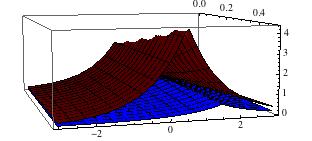
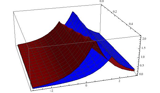
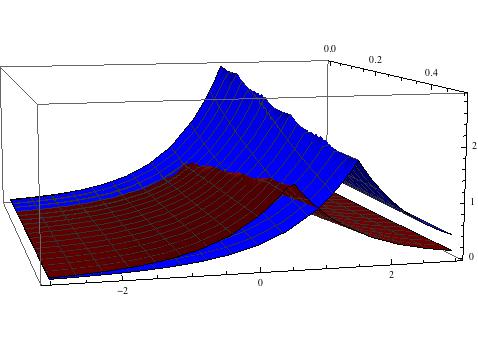
Figure 1: The figures, from left to right, show the function (22) with $\kappa=e$, $q_{0}=1$ and $p_{0}=1,\,2$, $3$, respectively. Function $u$ is represented in blue, whereas $v$ in red. The graphics were made with Mathematica by taking $(x,t)\in[0,1/2]\times[-3,3]$.

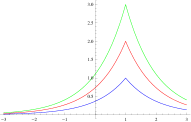
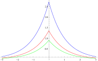
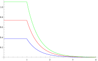
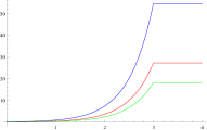
Figure 2: The first and second figures, from left to right, describe $u(x,0)$ and $v(x,0)$ as provided by (22) with $x\in[-3,3]$. The third and the fourth figures represent $u(2,t)$ and $v(2,t)$ for $t\in[0,4]$. In all cases $p_{0}\,P_{0}=\rme$ and $q_{0}=1$ and $Q_{0}=0$, whereas the values $p_{0}=1,\,2$ and $3$ correspond to blue, red and green, respectively.

5 Discussion

Our results in this paper show that the multidimensional generalisation (1) of the equation (2) exhibits a behaviour slightly different from the scalar case when $b>2$, and very different for $b=1$ and $b=2$. Case $b=2$ is particularly interesting and richer.

From the point of view of Lie symmetries, when $b\neq 2$ system (1) has the same classical symmetry algebra of (2), as follows by comparing with the results obtained in [9, 3]. On the contrary, when $b=2$, system (1) admits a $6$-dimensional classical symmetry algebra which extends the $5$-dimensional symmetry algebra admitted by the Novikov equation [7, 12, 3]. For instance, when $b=2$ the system (2) acquires the symmetry generator $X_{4}$ in (4). Although at the level of point symmetries we have a minor change of behaviour of (1) when compared with (2), we begin to have better evidence of the differences when we look for higher order symmetries. In this direction, the only case we find such symmetries for system (1) is just $b=2$, whereas equation (2), being integrable for $b=1$ and $b=2$, has higher order symmetries for these cases, see [8, 23, 35].

It has also been shown (see Theorem 4) that for $b=2$ system (1) can be embedded in a $4$-component system admitting an $\mathfrak{sl}(3,\mathbb{R})-$valued zero-curvature representation which generalizes a $4$-component system found in [32]. Indeed, the $4$-component system described in our paper is not contact equivalent to that obtained in [32].

With respect to conserved quantities, it is known that equation (2) admits, for any positive integer value of $b$, the first integral (actually, a Hamiltonian for $b=1$ and $b=2$)

$${\cal H}_{1}[u]=\int_{\mathbb{R}}\left(u^{2}+u_{x}^{2}\right)dx,$$ (25)

see [3, 8, 7, 10, 11, 23]. This integral corresponds to the Sobolev norm in $H^{1}(\mathbb{R})$ of the solutions $u$ of (2). Therefore, it is natural to expect that the bilinear form

$${\cal H}[u,v]=\int_{\mathbb{R}}\left(uv+u_{x}v_{x}\right)dx=\int_{\mathbb{R}}\left(vm+un\right)dx$$ (26)

would be a first integral of (1). Notice that, for the scalar case, the integral (25) can be derived by using the multiplier $u$ (in the sense of [1, 2, 3]) or the fact that (1) is strictly self-adjoint (in the sense of [24, 25]). In the latter case, this first integral is derived from the scaling generator $X^{b}$ in (3), see [7, 10, 26].

According to Table 1, the first integral (26) is derived as in the scalar case for $b=2$. However, (26) is a first integral only for $b=2$. Indeed, by multiplying the first equation of system (1) by $v$ and the second by $u$, simple manipulations yield the following relation:

$$\begin{array}[]{lcl}D_{t}(vm+un)&=&-(b+1)[u_{x}\,v^{b}\,m+v_{x}\,u^{b}\,n]\\ \\ &&-(u^{b-1}\,v^{2}\,m_{x}+v^{b-1}\,u^{2}\,n_{x})+(v_{t}\,m+u_{t}\,n).\end{array}$$ (27)

Hence, (27) provides a conservation law for (1) only for $b=2$, since just for this value of $b$ the right hand side of (27) is a total derivative with respect to $x$. Indeed, by computing the variational derivative of the right hand side of (27) one can see that this only happens for $b=2$. In this case (27) can be rewritten as

$$\begin{array}[]{l}D_{t}(vm+un)+D_{x}[2u^{2}(2v^{2}-v_{x}^{2}-vv_{xx})\\ \\ +u(4vu_{x}v_{x}-v_{tx}-2v^{2}u_{xx})+u_{t}v_{x}+u_{x}v_{t}-vu_{tx}-2v^{2}u_{x}^{2}]=0.\end{array}$$ (28)

Notice that in the degenerated case $u=v$ equation (27) provides a conservation law for any value of $b$, since its right hand side is always a total derivative with respect to $x$.

Still about conserved quantities of (1), in [15] it was shown that system (1) with $b=2$ has a Hamiltonian. In [30] and [31] it was also found a second Hamiltonian and proved that (1) with $b=2$ has a bi-Hamiltonian structure.

Finally, the most intriguing differences between the system (1) and the scalar equation (2) concern peakon solutions. Multi-peakon solutions of (1) can be found by solving system (12), which is in general a difficult task. However, 1-peakon solutions have been explicitly computed and show a noteworthy difference between 1-peakons of (1) and those of (2).

In the paper [15] the authors found the functions (23) as solutions for system (1) with $b=2$. These functions are $L^{p}(\mathbb{R})-$integrables, for each $p$, and, in particular, are in $L^{2}(\mathbb{R})$. However, we obtain a more general solution (22) which admits (23) as a particular case. These new solutions are $1$-peakons with non-constant amplitude and non-conservative norms in view of (24), unless $x_{0}=0$, which implies that $q_{0}$ and $Q_{0}$ are just the same as well as $q(t)=Q(t)$, see Theorem 9.

It is worth to notice that, if $x_{0}\neq 0$ in (22), then either one of the functions $u$ or $v$ blows up when $t\rightarrow\infty$. This can be easily checked in the case $x_{0}=q_{0}>0,\,p_{0}\,P_{0}>0$ and $Q_{0}=0$, since for curve $t\mapsto x(t)=p_{0}P_{0}e^{-|q_{0}|}t$ one has $|v(p_{0}P_{0}e^{-|q_{0}|}t,t)|\rightarrow\infty$ when $t\rightarrow\infty$. This is another way to foresee that the norms of the solutions are not conserved. Particularly, they are not squared integrable solutions. However, in spite of this unboundedness, Theorem 7 entails that the integral (26) is bounded for these $1$-peakons since $uv,\,u_{x}v_{x}\thicksim{\rm e}^{-|x-p_{0}\,P_{0}\,t|}$.

6 Acknowledgement

The authors are grateful to P. L. da Silva for doing the figures of this paper and for useful discussions that motivated us to consider $N$ and $M$ multipeakons in (9). The work of D. Catalano Ferraioli was partially supported by CNPq (grants no. $310577/2015-2$ and $422906/2016-6$). The work of I. L. Freire was partially supported by CNPq (grants no. $308516/2016-8$ and $404912/2016-8$). I. L. Freire would like to express his gratitude to the Departamento de Matemática – UFBA, where this work begun, for the warm hospitality.

References

References

- [1] S. Anco and G. Bluman, Direct construction method for conservation laws of partial differential equations. I. Examples of conservation law classifications, European J. Appl. Math., 13, 545–566, (2002).
- [2] S. Anco and G. Bluman, Direct construction method for conservation laws of partial differential equations. II. General treatment, European J. Appl. Math., 13, 567–585, (2002).
- [3] S. Anco, P. L. da Silva and I. L. Freire, A family of wave-breaking equations generalizing the Camassa-Holm and Novikov equations, J. Math. Phys., 56, paper 091506, (2015).
- [4] G. W. Bluman and S. Kumei, Symmetries and Differential Equations, Applied Mathematical Sciences 81, Springer, New York, (1989).
- [5] G. W. Bluman and S. Anco, Symmetry and Integration Methods for Differential Equations, Springer, New York, (2002).
- [6] G. Bluman, A. Cheviakov, S.C. Anco, Applications of Symmetry Methods to Partial Differential Equations, Springer Applied Mathematics Series 168, Springer, New York, (2010).
- [7] Y. Bozhkov, I. L. Freire and N. H. Ibragimov, Group analysis of the Novikov equation, Comp. Appl. Math., 33, 193–202, (2014).
- [8] R. Camassa and D. D. Holm, An integrable shallow water equation with peaked solitons, Phys. Rev. Lett., 71, 1661–1664, (1993).
- [9] P. A. Clarkson, E. L. Mansfield and T. J. Priestley, Symmetries of a class of nonlinear third-order partial differential equations, Math. Comput. Modelling., 25, 195–212, (1997).
- [10] P. L. da Silva and I. L. Freire, On certain shallow water models, scaling invariance and strict self-adjointness, Proceeding Series of the Brazilian Society of Computational and Applied Mathematics, (2015), DOI: /10.5540/03.2015.003.01.0022. See also, P. L. da Silva and I. L. Freire, Strict self-adjointness and shallow water models, e-print arXiv:1312.3992 (2013).
- [11] P. L. da Silva and I. L. Freire, An equation unifying both Camassa-Holm and Novikov equations, Proceedings of the 10th AIMS International Conference, (2015), DOI: 10.3934/proc.2015.0304.
- [12] P. L. da Silva and I. L. Freire, On the group analysis of a modified Novikov equation, Interdisciplinary Topics in Applied Mathematics, Modeling and Computational Science, 117 Springer Proceedings in Mathematics and Statistics, 161-166, (2015), DOI: 10.1007/978-3-319-12307-323.
- [13] A. Degasperis, D. D. Holm and A. N. W. Hone, A new integrable equation with peakon solutions, Theor. Math. Phys., 133, 1463–1474, (2002).
- [14] A. Fokas, Symmetries and integrability, Studies Appl. Math., 77, 253–229, (1987).
- [15] X. Geng and B. Xue, An extension of integrable peakon equations with cubic nonlinearity, Nonlinearity, 22, 1847–1856, (2009).
- [16] A. A. Himonas and C. Holliman, The Cauchy problem for the Novikov equation Nonlinearity, 25, 449–479, (2012).
- [17] A. A. Himonas and J. Holmes, Holder continuity of the solution map for the Novikov equation, J. Math. Phys., 54, paper 061501, (2013).
- [18] K. Grayshan and A. Himonas, Equations with peakon traveling wave solutions, Adv. Dyn. Syst. Appl., 8, 217–232, (2013).
- [19] A. Himonas and C. Holliman, The Cauchy problem for a generalized Camassa-Holm equation, Adv. Differ. Equations, 19, 161–260, (2014).
- [20] A. Himonas and D. Mantzavinos, An -family of equations with peakon traveling waves, Proc. Amer. Math. Soc., 144, 3797–3811, (2016).
- [21] D. D. Holm and M. F. Staley, Wave structure and nonlinear balances in a family of evolutionary PDEs, Siam. J. Appl. Dyn. Sys., 2, 323–380, (2003).
- [22] D. D. Holm and R. I. Ivanov, Multi-component generalizations of the CH equations: geometrical aspects, peakons and numerical examples, J. Phys. A: Math. Theor., 43, paper 492001, (2010)
- [23] A. N. W. Hone and J. P, Wang, Integrable peak on equations with cubic nonlinearities, J. Phys. A: Math. Theor., 41, 372002, 10 pp., (2008).
- [24] N. H. Ibragimov, A new conservation theorem, J. Math. Anal. Appl., 333, 311–328, (2007).
- [25] N. H. Ibragimov, Nonlinear self-adjointness and conservation laws, J. Phys. A: Math. Theor., 44, 432002, 8 pp., (2011).
- [26] N.H. Ibragimov, R.S. Khamitova, A. Valenti, Self-adjointness of a generalized Camassa-Holm equation, Appl. Math. Comp., 218, 2579–2583, (2011).
- [27] N. H. Ibragimov, Transformation groups and Lie algebras, World Scientific, (2013).
- [28] P. H. van der Kamp and J. Sanders, Almost integrable evolution equations, Selecta Mathematica, 8, 705–719, (2002).
- [29] J. Lenells, Conservation laws of the Camassa-Holm equation, J. Phys. A: Math. Gen., 38, 869–880, (2005).
- [30] N. Li and Q. P. Liu On bi-Hamiltonian structure of two-component Novikov equation, Phys. Lett. A, 377, 257–261, (2013).
- [31] H. Li, Y. Li and Y. Chen, Bi-hamiltonian structure of multi-component Novikov equation, J. Nonlin. Math. Phys., 21, 509–520, (2014).
- [32] N. Li, Q. P. Liu and Z. Popowicz, A four-component Camassa-Holm type hierarchy, J. Geom. Phys., 85, 29–39, (2014).
- [33] A. V. Mikhailov, Introduction, Lect. Notes Phys., 767, 1–18, (2009), DOI: 10.1007/978-3-540-88111-70.
- [34] A. V. Mikhailov and V. S. Novikov, Perturbative symmetry approach, J. Phys. A: Math. Gen., 35, 4775–4790, (2002).
- [35] V. S. Novikov, Generalizations of the Camassa-Holm equation, J. Phys. A: Math. Theor., 42, 342002, 14 pp., (2009).
- [36] P. J. Olver, Applications of Lie groups to differential equations, 2nd edition, Springer, New York, (1993).
- [37] Z. Qiao, A new integrable equation with cuspons and W/M-shape-peaks solitons, J. Math. Phys., 47, paper 112701, (2006).
- [38] L. Schwartz, Mathematics for the physical sciences, Dover, (2008) [English translation of L. Schwartz, Méthodes mathématiques pour les sciences physiques, (1966)].
- [39] A. M. Vinogradov, Local symmetries and conservation laws, Acta Appl. Math., 2, 21–78, (1984).