Multiscale Sub-grid Correction Method for Time-Harmonic High-Frequency Elastodynamics with Wavenumber Explicit Bounds

Abstract

The simulation of the elastodynamics equations at high-frequency suffers from the well known pollution effect. We present a Petrov–Galerkin multiscale sub-grid correction method that remains pollution free in natural resolution and oversampling regimes. This is accomplished by generating corrections to coarse-grid spaces with supports determined by oversampling lengths related to the $\log(k)$, $k$ being the wavenumber. Key to this method are polynomial-in-$k$ bounds for stability constants and related inf-sup constants. To this end, we establish polynomial-in-$k$ bounds for the elastodynamics stability constants in general Lipschitz domains with radiation boundary conditions in $\mathbb{R}^{3}$. Previous methods relied on variational techniques, Rellich identities, and geometric constraints. In the context of elastodynamics, these suffer from the need to hypothesize a Korn's inequality on the boundary. The methods in this work are based on boundary integral operators and estimation of Green's function's derivatives dependence on $k$ and do not require this extra hypothesis. We also implemented numerical examples in two and three dimensions to show the method eliminates pollution in the natural resolution and oversampling regimes, as well as performs well when compared to standard Lagrange finite elements.

1 Introduction

Modelling and simulating high-frequency wave propagation in complex media is a computationally demanding process. The need in applications to simulate wave propagation with accurate and robust numerical methods is wide ranging. In acoustics applications such as the automotive and aerospace industries, the need to understand sound propagation is critical for vibration control and consumer comfort. For more complex mechanical media, the acoustic (Helmholtz) equation is not sufficient to describe the real propagation of signals and waves. This is the case in subsurface seismic imaging applications, whereby attenuation from the elastic properties must be taken into account. The simulation of accurate signal propagation through the subsurface is utilized in calibrating the material properties in earth models and thus must be fast and robust. This is utilized in application domains ranging from environmental to petroleum exploration, and even mining engineering applications.

It has been known for many years that at high-frequency, using numerical methods in Helmholtz type problems yields a pollution effect in the solution if the mesh parameter, $h$, is able not to resolve the effects of high-frequency $k$. It is has been shown [2] that using a finite stencil completely eliminating the pollution effect is impossible for two or more space dimensions (while the authors of [2] were able to exhibit a pollution-free method in one space dimension). There are a wide range of methodologies and techniques for trying to combat the pollution error and here we mention only a few. A plane wave Lagrange multiplier technique is utilized in [45] for the mid-frequency range. Utilizing a Discontinuous Galerkin (DG) formulation for both $h$ and $hp$ the authors develop methods for high-frequency in [17, 18]. In the boundary integral method setting, asymptotic methods may be used [8]. By going to a fully DG context and computing an optimal test space, the authors in [48] are able to obtain a pollution free method in one space dimension. A breakthrough was achieved by relating the polynomial order $p$ to the frequency $k$ in a logarithmic way utilizing $hp$ methods in [37, 36]. In this work, we shall utilize a method based on the so-called Local Orthogonal Decomposition (LOD) [32].

The LOD method is based on utilizing quasi-interpolation operators to build a fine scale or detail space. Then, by forcing orthogonality an augmented coarse-space is constructed. However, the supports of these corrections to the original coarse-space are global. To make the scheme computationally efficient a truncation to local patch procedure is implemented. The errors of such a truncation can be carefully tracked [22, 32]. The method originally was conceived to handle elliptic problems with very rough and multiscale coefficients. However, since its inception it has seen generalizations to semi-linear equations [21, 20], oversampling methods [23], problems with microstructure [6], and parabolic problems [31], just to name a few. For this paper, we utilize the method's effective ability to eliminate pollution in optimal coarse-grid, $H$, and frequency, $k$, regimes [5, 19, 42]. Assuming polynomial-in-$k$ growth of stability and inf-sup constants of the continuous problem, and supposing patch truncations (oversampling) parameter $m$ of order $\log(k)$, we obtain a pollution free method in the resolution condition, $Hk\lesssim 1$ range.

However, polynomial-in-$k$ growth of stability constants is not guaranteed as trapping domains may yield constants of order $\exp(k),$ for certain frequency values [4, 7]. The study and calculation of the stability and related inf-sup constants and their dependence on $k$ is a vivid area of active research that dates back to the early works [39, 38, 46] as well as [16] . In the acoustic setting, given certain geometric and convexity conditions, the work of [34] gave polynomial (constant) bounds in $k$. Subsequent generalizations and extensions of these methods in the Helmholtz setting can be found in [12, 24, 25, 44, 3]. In general, these methods rely on variational techniques that utilize the special test function $x\cdot\nabla u$, Rellich identities, geometric constraints, and various boundary condition constraints. These methods have also been extended to the case of smooth weakly heterogeneous coefficients [5], although with serious constraints on coefficients that can be considered.

Prior to this work, a key issue in using this variational and Rellich identities method for the elastodynamics (elastic Helmholtz) case is the fact that the stress terms arrive on certain boundary integrals. In standard elasticity analysis, Korn's second inequality (see [33]) is employed to handle these terms in the interior of the domain. However, in the fundamental work of [12], to obtain gradient lower bounds on these stress terms a ``boundary'' Korn's inequality must be conjectured of the form

$$\left\lVert\frac{1}{2}\left(\nabla u+(\nabla u)^{T}\right)\right\rVert_{L^{2}(\partial\Omega)}^{2}\geq C\left(\left\lVert\nabla u\right\rVert_{L^{2}(\partial\Omega)}^{2}-\left\lVert u\right\rVert_{L^{2}(\partial\Omega)}^{2}\right),$$ (1.1)

for some boundary $\partial\Omega$. Here $\Omega\subset\mathbb{R}^{d},d=2,3.$ Although such a result may seem reasonable it is as yet unproven and must be assumed to obtain polynomial-in-$k$ bounds for the elastodynamics case.

However, in the recent works of [15, 37, 35, 44], a new technique is developed in the Helmholtz case without using the variational techniques and instead relying on boundary integral operators, estimates-in-$k$ of Green's functions, and Green's identity. These techniques make minimal (Lipschitz domain) geometric assumptions on the domain, but must be used for radiation (Robin type) boundary conditions. It is this technique that we use in this work for the elastodynamics case with radiation boundary conditions. The main theoretical contribution of this work is to show methods in [15, 37, 36] can be extended to the case of elastodynamics (elastic Helmholtz) and establish polynomial-in-$k$ bounds without the use of a conjectured boundary Korn's inequality (1.1) in $\mathbb{R}^{3}$. We finally mention the independent work [10], which establishes similar stability bounds (with sharper $k$-dependence but a slightly different geometric setting).

The proof of the polynomial bounds requires many auxiliary computations and results, so we sketch the organization of the proof and paper as follows. In Section 2, we present the problem set up of the elastodynamics equations with radiation boundary conditions in the frequency domain and its related variational forms. We then introduce the Green's function, $G_{k}$ and related potential operators. In this mechanics context, $G_{k}$ is referred to as the Kupradze matrix [29, 30]. We define the Newton potential, $N_{k}$ and present $k$-dependent estimates as in [37]. From here we obtain estimates for the single and double layer potentials, denoted $\widetilde{V}_{k},\widetilde{K}_{k},$ respectively. This is accomplished by employing a technique from [44], where layer potential estimates are obtained for nontrivial $k$. Then, we utilize standard a-priori and variational techniques, along with the ideas from [16, 15], where we write the solution via single and double layer potentials by Green's identity. Using the estimates for the layer potentials we obtain an estimate for $u$ in terms of known boundary norms of $u$ and $\sigma(u)\nu$. This gives polynomial-in-$k$ bounds as well as the related inf-sup constant.

In Section 3, we present the ideas of the multiscale sub-grid correction algorithm as in [5, 19, 42]. Here we present the algorithm as well as the basic error analysis. We implemented examples for both two and three dimensional examples and see that the method performs well in handling pollution effects when compared to the standard Lagrange finite elements.

Finally, the Appendix A is devoted to the proof of the main Newton potential estimates. The $k$-dependence of derivatives of Green's function (Kupradze matrix) is critical for the estimates in Section 2. We use the Fourier techniques to estimate the Green's function similar to [37]. The key observation, suggested by an anonymous reviewer in a previous version of the manuscript, is to notice the additional term of the Green's function has a cancellation in the leading order of the singularity. This observation greatly simplifies the analysis of a previous version by the authors. The Green's function estimate then yields estimates for $N_{k}$.

Standard notation on complex-valued Lebesgue and Sobolev spaces applies in this paper. The real and imaginary part of $z\in\mathbb{C}$ reads $\Re z$ and $\Im z$, respectively. The imaginary unit is denoted by $\mathbf{i}$ and the bar denotes complex conjugation $\bar{z}=\Re z-\mathbf{i}\Im z$. The analysis in this paper is explicit in the wavenumber $k$ and in the mesh-size parameters $H$ and $h$ of the finite element spaces. Generic constants, often denoted by $C$ and possibly having different values at different occurrences, are independent of those parameters. An inequality $A\leq CB$, will be frequently abbreviated by $A\lesssim B$. The notation $A\approx B$ means $A\lesssim B\lesssim A$. We focus on the regime of large wave numbers $k$ and will sometimes use that $k$ is sufficiently large.

2 Elastodynamic Equation in the Frequency Domain

In this section, we will introduce the governing equations for the three dimensional elastodynamic equation. Here we introduce the related variational form, as well as the critical Korn (in the interior of the domain) and Gårding inequalities. We will then prove the wavenumber explicit bounds for the solution and show that we obtain frequency $k$-polynomial bounds of the solution given a radiation boundary condition on a bounded connected Lipschitz domain. From this we are able to obtain an estimate for the inf-sup stability constant utilized heavily in our multiscale numerical algorithm.

2.1 Elastodynamics Governing Equations

We now begin the problem setting. First, let $\Omega\subset\mathbb{R}^{3}$ be a bounded open connected Lipschitz domain in $\mathbb{R}^{3}$ and take $f\in L^{2}(\Omega)^{3}$ and $g\in L^{2}(\partial\Omega)^{3}$. We suppose that $u$ satisfies the elastodynamic equation (time-harmonic elastic wave equation in the frequency domain) with radiation boundary conditions. We suppose that our material satisfies a homogeneous isotropic stress tensor

$$\sigma(u)=2\mu\varepsilon(u)+\lambda\text{tr}(\varepsilon(u))=\mu(\nabla u+(\nabla u)^{T})+\lambda\text{div}(u)I,$$ (2.1)

where the symmetric gradient is given by $\varepsilon(u)=(\nabla u+(\nabla u)^{T})/2$, $I$ is the identity matrix, and superscript $T$ denotes transpose. We let $u=(u^{(1)},u^{(2)},u^{(3)})$ be the solution of the following governing equations

$$-\text{div}(\sigma(u))-k^{2}u =f\text{ in }{\Omega},$$ (2.2a)

$$\sigma(u)\nu+\mathbf{i}ku =g\text{ on }\partial\Omega$$ (2.2b)

where $\nu$ is the outward normal. Note that this is equivalent to the Lamé equations

$$-\mu\Delta u-(\lambda+\mu)\nabla(\text{div}(u))-k^{2}u =f\text{ in }{\Omega},$$

$$\lambda\text{div}(u)\nu+\mu(\nabla u+(\nabla u)^{T})\nu+\mathbf{i}ku =g\text{ on }\partial\Omega.$$

Here $\lambda$ and $\mu$, are the Lamé constants with $\mu>0$ and $\lambda>-2\mu/3$ [13, 27]. We require further that $\lambda+2\mu>0$ for strong ellipticity [33, p. 297]. The boundary condition is the elastodynamic analogue of the Robin boundary condition $\nabla u\cdot\nu+\mathbf{i}ku=g$ in the acoustic Helmholtz context. In elasticity, a traction boundary condition is required, here we define the traction conormal as

$$\frac{\partial u}{\partial\nu}:=\sigma(u)\nu=\lambda\text{div}(u)\nu+\mu(\nabla u+(\nabla u)^{T})\nu,$$ (2.3)

which for notational brevity we will often denote $\partial_{\nu}u$. The corresponding variational form can be arrived at via the Betti formula [26], multiplying (2.2) by $\bar{v}$ and integrating we obtain

$$-\int_{{\Omega}}\text{div}(\sigma(u))\cdot\bar{v}dx-\int_{{\Omega}}k^{2}u\cdot\bar{v}dx=\int_{{\Omega}}\sigma(u):\nabla\bar{v}dx-\int_{\partial{\Omega}}\sigma(u)\nu\bar{v}ds-\int_{{\Omega}}k^{2}u\cdot\bar{v}dx$$

$$=\int_{{\Omega}}\left(\mu(\nabla u+(\nabla u)^{T})+\lambda\text{div}(u)I\right):\nabla\bar{v}dx-\int_{\partial{\Omega}}(g-\mathbf{i}ku)\cdot\bar{v}ds-\int_{{\Omega}}k^{2}u\cdot\bar{v}dx.$$

Here we have full contraction denoted by $A:B=\sum_{ij}A_{ij}B_{ij}$. Thus, using the identity $\text{div}(u)I:\nabla\bar{v}=\text{div}(u)\text{div}(\bar{v})$, and $2(\nabla u+(\nabla u)^{T}):\nabla\bar{v}=(\nabla u+(\nabla u)^{T}):(\nabla\bar{v}+(\nabla\bar{v})^{T}),$ we may write the following variational form. Find $u\in(H^{1}({\Omega}))^{3},$ satisfying

$$\Phi(u,\bar{v})=F(v)\text{ for all }\bar{v}\in(H^{1}({\Omega}))^{3},$$ (2.4)

where $\Phi(u,\bar{v})=\Phi_{{\Omega}}(u,\bar{v})+\Phi_{\partial{\Omega}}(u,\bar{v})$ and $F$ are given by

$$\Phi_{{\Omega}}(u,\bar{v})=\int_{{\Omega}}\left(\lambda\text{div}(u)\text{div}(\bar{v})+{2\mu}\varepsilon(u):\varepsilon(v)-k^{2}u\cdot\bar{v}\right)dx$$ (2.5a)

$$\Phi_{\partial{\Omega}}(u,\bar{v})=\mathbf{i}k\int_{\partial{\Omega}}u\cdot\bar{v}ds,\qquad F(v)=\int_{\partial{\Omega}}g\cdot\bar{v}ds+\int_{{\Omega}}f\cdot\bar{v}dx.$$ (2.5b)

Here $dx$ is the standard Lebesgue volume measure, and $ds$ the standard Lebesgue surface measure. We will denote $\left\lVert\cdot\right\rVert_{L^{2}({\Omega})}$ and $\left\lVert\cdot\right\rVert_{H^{s}({\Omega})}$, $s=1,2$, to be the standard Sobolev norms. When there is no ambiguity we will not differentiate between the vector norms and scalar norms.

Recall, for the open bounded Lipschitz domain $\Omega\subset\mathbb{R}^{3}$, Korn's second inequality (in the interior) [33]

$$\left\lVert\varepsilon(u)\right\rVert_{L^{2}(\Omega)}^{2}\geq c_{\mathrm{Korn}}\left\lVert\nabla u\right\rVert_{L^{2}(\Omega)}^{2}-C_{\mathrm{Korn}}\left\lVert u\right\rVert_{L^{2}(\Omega)}^{2}.$$ (2.6)

We have for some $C,c$ positive and independent of $k$, that

$$\Re\Phi_{{\Omega}}(u,\bar{u}) =2\mu\left\lVert\varepsilon(u)\right\rVert_{L^{2}({\Omega})}^{2}+\lambda\left\lVert\text{div}(u)\right\rVert_{L^{2}({\Omega})}^{2}-k^{2}\left\lVert u\right\rVert_{L^{2}({\Omega})}^{2}$$ (2.7)

$$\geq C\left\lVert\nabla u\right\rVert_{L^{2}({\Omega})}^{2}-(c+k^{2})\left\lVert u\right\rVert_{L^{2}({\Omega})}^{2}.$$

Indeed, we see that this is the Gårding's inequality on $(H^{1}({\Omega}))^{3}$. With an argument analogous to that of [34, Sect. 8.1] one can show that (2.4) is uniquely solvable. We will make the $k$-dependence precise in Theorem 2.7 below.

2.2 Green's Functions and Potentials' Estimates

In this subsection, we will introduce the ideas and notation to analyze the first and second layer potentials in elastodynamics. We will introduce the Green's function (in this setting it is the Kupradze matrix) and related boundary and Newton potentials. These, via Somigliana's formula (Green's identiy), give a representation for the solution of the elastodynamics equation.

We begin with some notation following the style introduced in [13] and [35]. As above, let $\Omega\subset\mathbb{R}^{3}$ be a bounded, open, connected Lipschitz domain in $\mathbb{R}^{3}$. Finally, we suppose the convention [35] that $k\geq k_{0}>0$ for some fixed $k_{0}$. As seen in Section 2.3, Theorem 2.8, $k_{0}$ is related to the Korn's second inequality constant $C_{\text{Korn}}$, and depends only on the domain and material parameters, but not on $k$. In general, we are considered here with high-frequency (large $k$) problems. We now define the Green's function, or in this setting often referred to as the Kupradze matrix, corresponding to (2.2a). The Green's function is the fundamental solution to the equation

$$-\text{div}\left(\sigma\left(G_{k}(x-y)\right)\right)-k^{2}G_{k}(x-y) =\delta(x-y)\text{ in }{\Omega},$$ (2.8)

or expanded out into the Lamé equations form

$$-\mu\Delta G_{k}(x-y)-(\lambda+\mu)\nabla(\text{div}(G_{k}(x-y)))-k^{2}G_{k}(x-y) =\delta(x-y)\text{ in }{\Omega}$$ (2.9)

for the Dirac distribution $\delta$.

Remark 2.1.

There are many ways to obtain the Green's function of the above system. For $d=2,3$, the Green's function can be obtained as in [28] via Hörmander's method of parametrics and derived via Radon transforms in [47]. For a complete treatment of this subject we refer the readers to [29, 30].

Letting $k_{1}^{2}=k^{2}(\lambda+2\mu)^{-1}\,,\,k_{2}^{2}=k^{2}\mu^{-1}$, for $i,j=1,2,3$, we write the Green's function as

$$(G_{k}(r))_{ij} =\frac{1}{4\pi\mu}\left(\delta_{ij}\frac{e^{\mathbf{i}k_{2}r}}{r}+\frac{1}{k_{2}^{2}}\frac{\partial^{2}}{\partial x_{i}\partial x_{j}}\left(\frac{e^{\mathbf{i}k_{2}r}}{r}-\frac{e^{\mathbf{i}k_{1}r}}{r}\right)\right),$$ (2.10a)

$$(G^{E}_{k}(r))_{ij} =\frac{1}{4\pi\mu}\left(\frac{1}{k_{2}^{2}}\frac{\partial^{2}}{\partial x_{i}\partial x_{j}}\left(\frac{e^{\mathbf{i}k_{2}r}}{r}-\frac{e^{\mathbf{i}k_{1}r}}{r}\right)\right),$$ (2.10b)

$$(G^{H}_{k}(r))_{ij} =\frac{1}{4\pi\mu}\left(\delta_{ij}\frac{e^{\mathbf{i}k_{2}r}}{r}\right),$$ (2.10c)

where $r=|x|$, is the standard Euclidean distance in spherical coordinates. Note that the elastic rotational term (2.10b) is smoother than it first appears. Indeed, note that $\left(\frac{e^{\mathbf{i}k_{2}r}}{r}-\frac{e^{\mathbf{i}k_{1}r}}{r}\right)\to 0$ as $r\to 0$, so that the leading order singularity is cancelled.

Remark 2.2.

Note that a two-dimensional representation for the elastodynamics Green's function exists. Indeed, from [28], we have

$$(G_{k}(r))_{ij}=\frac{\mathbf{i}}{4\mu}\left(\delta_{ij}H_{0}^{(1)}(k_{2}r)+\frac{1}{k_{2}^{2}}\frac{\partial^{2}}{\partial x_{i}\partial x_{j}}\left(H_{0}^{(1)}(k_{2}r)-H_{0}^{(1)}(k_{1}r)\right)\right),$$

where $H_{0}^{(1)}$ are zero order Hankel functions of the first kind. We expect that similar to [37], the following estimates hold for the two-dimensional, but leave this to future investigations due to the extra technical difficulties in handling Hankel functions as opposed to merely exponential functions of the form $\exp(\mathbf{i}kr)/r$.

The Newton potential for $f\in(L^{2}({\Omega}))^{3}$ with compact support in $\mathbb{R}^{3}$, is given by

$$(N_{k}(f))(x)=\int_{{\Omega}}G_{{k}}(x-y)f(y)dy,\text{ for }x\in{\Omega}.$$ (2.11)

Here we use the notation to mean $(N_{k}(f))_{i}=\sum_{j=1}^{3}\int_{{\Omega}}(G_{k})_{ij}(x-\cdot)f_{j}dy,i=1,2,3,$ and similarly for the operators defined below. We further define the layer potential operators as in [27] and [35] for $\varphi\in(L^{2}(\partial\Omega))^{3}$ and $x\in{\Omega}$ as

$$\widetilde{V}_{k}(\varphi)(x):=\int_{\partial{\Omega}}G_{{k}}(x-y)\varphi(y)ds_{y},\hskip 7.22743pt\widetilde{K}_{k}(\varphi)(x):=\int_{\partial{\Omega}}\partial_{\nu_{y}}G_{{k}}(x-y)\varphi(y)ds_{y},$$ (2.12)

here $\partial_{\nu_{y}},$ to denote the traction conormal, (2.3), with respect to $y$.

We then have a representation formula for (2.2) in the interior of the domain given by (2.13) below. This is the so-called Somigliana's formula (Green's identity in matrix form) [28, §1.6.2, p. 25], which we briefly describe here. Denote the operator corresponding to elastodynamics as ${\mathcal{L}}_{k}=-\mu\Delta-(\lambda+\mu)\nabla\text{div}-k^{2}$. From the Green's identity we have for $u$ a solution to (2.2) for $f=0$

$$\int_{{\Omega}}\left(G_{k}(x-y){\mathcal{L}}_{k}u(y)-{\mathcal{L}}_{k}G_{k}(x-y)u(y)\right)dy=\int_{\partial{\Omega}}\left(-G_{k}(x-y)\partial_{\nu_{y}}u(y)+\partial_{\nu_{y}}G_{k}(x-y)u(y)\right)ds_{y}.$$

Hence, we have the solution representation as

$$u(x)=\int_{\partial{\Omega}}\left(G_{k}(x-y)\partial_{\nu_{y}}u(y)-\partial_{\nu_{y}}G_{k}(x-y)u(y)\right)ds_{y},\,x\in{\Omega}.$$

Finally, (2.2) has a single layer and double layer potential representation of the form

$$u(x) =\widetilde{V}_{k}(\sigma(u)\nu)(x)-\widetilde{K}_{k}(u)(x),\,x\in{\Omega},$$ (2.13)

where $\sigma(u)\nu$ is defined via (2.3).

The above potentials satisfy the following $k$-dependent bounds.

Theorem 2.3 (Newton potential estimates).

Let $f\in(L^{2}({\Omega}))^{3},$ for the Newton potential (2.11) we have the estimate

$$k^{-1}{\left\lVert N_{k}(f)\right\rVert}_{H^{2}({\Omega})}+{\left\lVert N_{k}(f)\right\rVert}_{H^{1}({\Omega})}+k{\left\lVert N_{k}(f)\right\rVert}_{L^{2}({\Omega})}\leq C{\left\lVert f\right\rVert}_{L^{2}({\Omega})},$$ (2.14)

where $C>0$ is independent of $k$ and depends only on $\Omega,\mu,\lambda$.

• See Appendix A. ∎

With the Newton potential estimate, Theorem 2.3, we can establish the following layer potential estimates.

Lemma 2.4 (layer potential estimates).

The layer potential operators $\widetilde{V}_{k}$ and $\widetilde{K}_{k}$ defined in (2.12) satisfy, for any $\varphi\in(L^{2}(\partial\Omega))^{3}$, the estimates

$$\|\widetilde{V}_{k}(\varphi)\|_{L^{2}(\Omega)}\leq Ck^{-1/2}\|\varphi\|_{L^{2}(\partial\Omega)}\quad\text{and}\quad\|\widetilde{K}_{k}(\varphi)\|_{L^{2}(\Omega)}\leq Ck^{1/2}\|\varphi\|_{L^{2}(\partial\Omega)}.$$

• The proof is very similar to that of [44, Lemma 4.3] and we briefly show it here for completeness and self-consistent reading. Recall the Newton potential $N_{k}$ from (2.11) whose adjoint $N_{k}^{\prime}$ is given by

  $$(N_{k}^{\prime}(f))(x)=\int_{{\Omega}}\overline{G_{{k}}(x-y)}f(y)dy,\text{ for }x\in{\Omega},$$

  and satisfies $N^{\prime}_{k}(f)=\overline{N_{k}(\bar{f})}$. With the definitions (2.12) this leads to the identity

  $$\int_{\Omega}\widetilde{V}_{k}(\varphi)(x)\overline{f(x)}\,dx=\int_{\partial\Omega}\varphi(x)\overline{N_{k}^{\prime}(f)(x)}\,ds_{x}.$$

  The multiplicative trace inequality therefore shows

  $$\int_{\Omega}\widetilde{V}_{k}(\varphi)(x)\overline{f(x)}\,dx\leq\|\varphi\|_{L^{2}(\partial\Omega)}\|N_{k}^{\prime}f\|_{L^{2}(\partial\Omega)}\leq\|\varphi\|_{L^{2}(\partial\Omega)}\|N_{k}^{\prime}f\|_{L^{2}(\Omega)}^{1/2}\|N_{k}^{\prime}f\|_{H^{1}(\Omega)}^{1/2}.$$

  The Newton potential estimate (2.14) from Theorem 2.3 and the identity $N^{\prime}_{k}(f)=\overline{N_{k}(\bar{f})}$ therefore yield

  $$\int_{\Omega}\widetilde{V}_{k}(\varphi)(x)\overline{f(x)}\,dx\leq Ck^{-1/2}\|\varphi\|_{L^{2}(\partial\Omega)}\|f\|_{L^{2}(\Omega)}.$$

  Choosing $f=\widetilde{V}_{k}(\varphi)$ gives the first asserted estimate. Analogous computations for the double-layer potential read

  $$\int_{\Omega}\widetilde{K}_{k}(\varphi)(x)\overline{f(x)}\,dx\int_{\partial\Omega}\varphi(x)\overline{\partial_{\nu}N_{k}^{\prime}(f)(x)}\,ds_{x}\leq\|\varphi\|_{L^{2}(\partial\Omega)}\|N_{k}^{\prime}f\|_{H^{1}(\Omega)}^{1/2}\|N_{k}^{\prime}f\|_{H^{2}(\Omega)}^{1/2}$$

  and the combination with (2.14) implies

  $$\int_{\Omega}\widetilde{K}_{k}(\varphi)(x)\overline{f(x)}\,dx\leq Ck^{1/2}\|\varphi\|_{L^{2}(\partial\Omega)}\|f\|_{L^{2}(\Omega)}.$$

  The choice $f=\widetilde{K}_{k}(\varphi)$ then proves the second claimed estimate. ∎

2.3 $k$-Polynomial Growth of the Stability Constant

Here we present the main $k$-growth estimates of this work. We establish polynomial growth of the stability constant with respect to wavenumber $k$ for system (2.2). We will first require a few auxiliary lemmas similar to those obtained for the Helmholtz case in [15, 44]. Throughout this section, we will use the following notation

$$\left\lVert u\right\rVert_{1,k}:=\left({\left\lVert\nabla u\right\rVert}_{L^{2}({\Omega})}^{2}+k^{2}{\left\lVert u\right\rVert}_{L^{2}({\Omega})}^{2}\right)^{1/2}.$$

Lemma 2.5.

Let ${\Omega}\subset\,\mathbb{R}^{3}$ be a bounded, open, connected Lipschitz domain. Let $u\in(H^{1}({\Omega}))^{3}$ be a solution to (2.2) with $f=0$ with $g\in(L^{2}(\partial{\Omega}))^{3}$. Then,

$$\|u\|_{L^{2}(\partial\Omega)}\leq k^{-1}\|g\|_{L^{2}(\partial\Omega)}\quad\text{and}\quad\|\sigma(u)\nu\|_{L^{2}(\partial\Omega)}\leq\|g\|_{L^{2}(\partial\Omega)}.$$

• As in [9, 15], taking $v=u$ in (2.4), taking imaginary parts, and using the impedance boundary condition $\sigma(u)\cdot\nu=g-\mathbf{i}ku$ on $\partial\Omega$ we arrive at

  $$k\|u\|_{L^{2}(\partial\Omega)}^{2}=\Im\int_{\partial\Omega}g\cdot\bar{u}\,ds=\Im\int_{\partial\Omega}(\sigma(u)\nu+\mathbf{i}ku)\cdot\bar{u}\,ds.$$

  The first of these identities and the Cauchy inequality result in the first stated estimate. The identity plus elementary manipulations furthermore show

  $$0=\Im\int_{\partial\Omega}(\sigma(u)\nu)\cdot\bar{u}\,ds=-\frac{1}{k}\Re\int_{\partial\Omega}(\sigma(u)\nu)\cdot(\overline{\mathbf{i}ku})\,ds$$

  Inserting the impedance boundary condition for $\overline{\mathbf{i}ku}$ proves the second claimed estimate. ∎

For the next lemma, we will need the representation of the solution of (2.2) of the form (2.13), that is often referred to as Somigliana's in this context. Here, $\widetilde{V}_{k}$ and $\widetilde{K}_{k}$ are the layer potentials defined in Subsection 2.2.

Lemma 2.6.

Let ${\Omega}\subset\,\mathbb{R}^{3}$ be a bounded open, connected Lipschitz domain. Let $u\in(H^{1}({\Omega}))^{3}$ be a solution to (2.2) with $f=0$ and $g\in(L^{2}(\partial\Omega))^{3}$. Then, we have the following estimate

$$\left\lVert u\right\rVert_{1,k} \leq Ck^{1/2}\|g\|_{L^{2}(\partial\Omega)}.$$

• As in [44], we use Somigliana's formula (2.13) and the following estimates for the layer potentials from Lemma 2.4

  $$\|\widetilde{V}_{k}(\varphi)\|_{L^{2}(\Omega)}\leq Ck^{-1/2}\|\varphi\|_{L^{2}(\partial\Omega)}\quad\text{and}\quad\|\widetilde{K}_{k}(\varphi)\|_{L^{2}(\Omega)}\leq Ck^{1/2}\|\varphi\|_{L^{2}(\partial\Omega)}$$

  to conclude

  $$\|u\|_{L^{2}(\Omega)}\leq Ck^{-1/2}\|\sigma(u)\nu\|_{L^{2}(\partial\Omega)}+k^{1/2}\|u\|_{L^{2}(\partial\Omega)}.$$

  Combining this with Lemma 2.5 finally implies the $L^{2}$ bound

  $$\|u\|_{L^{2}(\Omega)}\leq Ck^{-1/2}\|g\|_{L^{2}(\partial\Omega)}.$$

  Relations (2.7) and (2.4) and $k\gtrsim 1$ with the Cauchy inequality prove

  $$C\|\nabla u\|_{L^{2}(\Omega)}^{2}\leq(k^{2}+c)\|u\|_{L^{2}(\Omega)}^{2}+\Re F(u)\lesssim k^{2}\|u\|_{L^{2}(\Omega)}^{2}+\|g\|_{L^{2}(\partial\Omega)}\|u\|_{L^{2}(\partial\Omega)}.$$

  Applying Lemma 2.5 and inserting the above $L^{2}$ bound concludes the proof. ∎

We now state and prove our main theorem.

Theorem 2.7.

Let ${\Omega}\subset\,\mathbb{R}^{3}$ be a bounded open, connected Lipschitz domain. Let $u\in(H^{1}({\Omega}))^{3}$ be a solution to (2.2), with $g\in(L^{2}(\partial{\Omega}))^{3}$ and $f\in(L^{2}({\Omega}))^{3}$. Then, there exists a constant $C>0$ independent of $k$, such that

$$\left\lVert u\right\rVert_{1,k}\leq C\left(k^{1/2}{\left\lVert g\right\rVert}_{L^{2}(\partial\Omega)}+k{\left\lVert f\right\rVert}_{L^{2}({\Omega})}\right).$$

• Taking the same approach as [15, 44], we transform the right hand side $f$ to the boundary. We define $u_{0}=G_{k}*f$ (extending $f$ to zero outside ${\Omega})$, where $G_{k}$ is the Green's function corresponding to (2.2), written explicitly in Subsection 2.2, (2.10a). We know from Theorem 2.3 that

  $$k^{-1}{\left\lVert u_{0}\right\rVert}_{H^{2}({\Omega})}+{\left\lVert u_{0}\right\rVert}_{H^{1}({\Omega})}+k{\left\lVert u_{0}\right\rVert}_{L^{2}({\Omega})}\leq C{\left\lVert f\right\rVert}_{L^{2}({\Omega})}.$$ (2.15)

  Writing $w=u-u_{0}$, we obtain

  $$-\text{div}(\sigma(w))-k^{2}w =0\text{ in }{\Omega},$$ (2.16a)

  $$\sigma(w)\nu+\mathbf{i}kw =g-(\sigma(u_{0})\nu+\mathbf{i}ku_{0})=:\tilde{g}\text{ on }\partial\Omega.$$ (2.16b)

  Using the multiplicative trace inequality on $\tilde{g}$, we obtain

  $${\left\lVert\tilde{g}\right\rVert}_{L^{2}(\partial\Omega)}\leq C\left({\left\lVert g\right\rVert}_{L^{2}(\partial\Omega)}+\left\lVert u_{0}\right\rVert^{1/2}_{H^{2}({\Omega})}\left\lVert u_{0}\right\rVert^{1/2}_{H^{1}({\Omega})}+k\left\lVert u_{0}\right\rVert^{1/2}_{H^{1}({\Omega})}\left\lVert u_{0}\right\rVert^{1/2}_{L^{2}({\Omega})}\right)$$

  $$\leq C\left({\left\lVert g\right\rVert}_{L^{2}(\partial\Omega)}+k^{1/2}{\left\lVert f\right\rVert}_{L^{2}({\Omega})}\right).$$

  The combination of this bound with Lemma 2.6 results in

  $$\left\lVert w\right\rVert_{1,k} \leq Ck^{1/2}\|\tilde{g}\|_{L^{2}(\partial\Omega)}\leq C\left(k^{1/2}\|\tilde{g}\|_{L^{2}(\partial\Omega)}+k\|f\|_{L^{2}(\Omega)}\right).$$

  Including the Newton potential bounds (2.15), we obtain our estimate. ∎

We now are in a position to derive the so-called inf-sup condition also derived in the same way as [5, 15]. The proof will make use of the unique solvability in the case of constant material coefficients, see the discussion at the end of §2.1.

Theorem 2.8.

Let ${\Omega}\subset\,\mathbb{R}^{3}$ be a bounded open, connected Lipschitz domain. Then there exists a $C>0$ independent of $k$, such that the variational form $\Phi$ in (2.4), satisfies

$$\inf_{0\neq u\in H^{1}({\Omega})^{3}}\sup_{0\neq v\in H^{1}({\Omega})^{3}}\frac{\Re\Phi(u,\bar{v})}{\left\lVert u\right\rVert_{1,k}\left\lVert v\right\rVert_{1,k}}\geq Ck^{-2}.$$

• Let $u\in H^{1}({\Omega})^{3}$ be given. As in [15] we define an auxiliary solution $z\in H^{1}({\Omega})^{3}$ satisfying

  $$\Phi(w,\bar{z})=2k^{2}(w,u)_{L^{2}({\Omega})}\quad\text{for all }w\in H^{1}(\Omega)^{3},$$ (2.17)

  and thus, by Theorem 2.7, $\left\lVert z\right\rVert_{1,k}\leq Ck{\left\lVert k^{2}u\right\rVert}_{L^{2}({\Omega})}\leq Ck^{3}{\left\lVert u\right\rVert}_{L^{2}({\Omega})}$. Letting $v=u+z$, and using the relation (2.17), we obtain

  $$\Re\Phi(u,\bar{v})=\Re\Phi(u,\bar{u})+\Re\Phi(u,\bar{z})=\Re\Phi(u,\bar{u})+2k^{2}(u,u)_{L^{2}({\Omega})}.$$

  Then, applying Korn's second inequality (2.6), we obtain

  $$\Re\Phi(u,\bar{v})=\Re\Phi(u,\bar{u})+2\int_{{\Omega}}k^{2}|u|^{2}dx =\int_{{\Omega}}\left(\lambda|\text{div}(u)|^{2}+{2\mu}|\varepsilon(u)|^{2}\right)dx+\int_{{\Omega}}k^{2}|u|^{2}dx$$

  $$\geq c\left\lVert\nabla u\right\rVert_{L^{2}(\Omega)}^{2}+(k^{2}-C)\left\lVert u\right\rVert_{L^{2}(\Omega)}^{2}\geq C\left\lVert u\right\rVert^{2}_{1,k},$$

  where again we used $C\lesssim k^{2}$. Finally, using the bound $\left\lVert v\right\rVert_{1,k}=\left\lVert u+z\right\rVert_{1,k}\leq Ck^{2}\left\lVert u\right\rVert_{1,k}$, we have

  $$\Re\Phi(u,v)\geq C\left\lVert u\right\rVert^{2}_{1,k}\geq Ck^{-2}\left\lVert u\right\rVert_{1,k}\left\lVert v\right\rVert_{1,k}.$$

  ∎

3 Multiscale Method

In this section we describe the application of the multiscale Petrov–Galerkin method (msPGFEM or msPG method) from [5, 19, 42] to the elasticity setting. This method is based on ideas in an algorithm developed for homogenization problems in [6, 23, 32] also known as Localized Orthogonal Decomposition. The ideas have been adapted to the Helmholtz problem for homogeneous coefficients in [42], and later presented in the Petrov–Galerkin framework [5, 19, 41].

3.1 Meshes and Data Structures

We begin with the basic notation needed regarding the relevant mesh and data structures. We keep the presentation general and will link it back to the elastodynamics case as we proceed. Let $\mathcal{T}_{H}$ be a shape-regular partition of $\Omega$ into intervals, parallelograms, parallelepipeds for $d=1,2,3$, respectively, such that $\bigcup\mathcal{T}_{H}=\overline{\Omega}$ and any two distinct $T,T^{\prime}\in\mathcal{T}_{H}$ are either disjoint or share exactly one lower-dimensional hyper-face (that is a vertex or an edge for $d\in\{2,3\}$ or a face for $d=3$). We suppose the mesh is quasi-uniform. For simplicity, we are considering quadrilaterals (resp. hexahedra) with parallel faces.

Given any subdomain $S\subset\overline{\Omega}$, we define its neighborhood to be

$$\omega(S):=\operatorname{int}\Big{(}\cup\{T\in\mathcal{T}_{H}\,:\,T\cap\overline{S}\neq\emptyset\}\Big{)}.$$

Furthermore, we introduce for any $m\geq 2$ the patch extensions

$$\omega^{1}(S):=\omega(S)\qquad\text{and}\qquad\omega^{m}(S):=\omega(\omega^{m-1}(S)).$$

Note that the shape-regularity implies that there is a uniform bound denoted $C_{\mathrm{ol},m}$, on the number of elements in the $m$th-order patch, $\#\{K\in\mathcal{T}_{H}\,:\,K\subset\overline{\omega^{m}(T)}\}\leq C_{\mathrm{ol},m}$ for all ${T\in\mathcal{T}_{H}}$. We will abbreviate $C_{\mathrm{ol}}:=C_{\mathrm{ol},1}$. The assumption that the coarse-scale mesh $\mathcal{T}_{H}$ is quasi-uniform implies that $C_{\mathrm{ol},m}$ depends polynomially on $m$. The global mesh-size is $H:=\max\{\operatorname{diam}(T):T\in\mathcal{T}_{H}\}$.

We will denote $Q_{1}(\mathcal{T}_{H})$ to be the space of piecewise bilinear. degree less than or equal to $1$. The space of globally continuous piecewise first-order polynomials is then given by $\mathcal{S}^{1}(\mathcal{T}_{H}):=C^{0}(\Omega)\cap Q_{1}(\mathcal{T}_{H}),$ and by incorporating the Dirichlet condition we arrive at the standard $Q_{1}$ finite element space denoted here as

$$V_{H}:=[\mathcal{S}^{1}(\mathcal{T}_{H})]^{d}\cap V$$

where $V$ denotes the energy space from see §3.2 below. We use quadrilateral/hexahedral elements for the ease of presentation, but the results remain valid for piecewise affine finite elements over simplicial partitions.

To construct our fine-scale and, thus, multiscale spaces we will need to define a coarse-grid quasi-interpolation operator. For simplicity of presentation,we suppose here that this quasi-interpolation is also projective. We let $I_{H}:V\to V_{H}$ be a surjective quasi-interpolation operator that acts as a stable quasi-local projection in the sense that $I^{2}_{H}=I_{H}$ and that for any $T\in\mathcal{T}_{H}$ and all $v\in V$ the following local stability result holds

$$H^{-1}\|v-I_{H}v\|_{L^{2}(T)}+\|\nabla I_{H}v\|_{L^{2}(T)}\leq C_{I_{H}}\|\nabla v\|_{L^{2}(\omega(T))}.$$ (3.1)

Under the mesh condition that

$$kH\lesssim 1$$ (3.2)

is bounded by a generic constant, this implies stability in the $\|\cdot\|_{V}$ norm

$$\|I_{H}v\|_{V}\leq C_{I_{H},V}\|v\|_{V}\quad\text{for all }v\in V,$$ (3.3)

with a $k$-independent constant $C_{I_{H},V}$. One possible choice and which we use in our implementation of the method, is to define $I_{H}:=E_{H}\circ\Pi_{H}$, where $\Pi_{H}$ is the piecewise $L^{2}$ projection onto $Q_{1}(\mathcal{T}_{H})$ and $E_{H}$ is the averaging operator that maps $Q_{1}(\mathcal{T}_{H})$ to $V_{H}$ by assigning to each free vertex the arithmetic mean of the corresponding function values of the neighbouring cells.

3.2 The Variational Setting

Let $\Omega\subset\mathbb{R}^{d}$ for $d=2$ or $d=3$ be a bounded polygonal Lipschitz domain with disjoint boundary portions $\Gamma_{R}$, $\Gamma_{D}$, $\Gamma_{N}$ and define the energy space $V:=\{v\in(H^{1}(\Omega))^{d}:v|_{\Gamma_{D}}=0\}$ equipped with the norm $\|\cdot\|_{V}:=\sqrt{k^{2}\|\cdot\|_{L^{2}(\Omega)}^{2}+\|\mathfrak{C}^{1/2}\varepsilon\cdot\|_{L^{2}(\Omega)}^{2}}$ (which is, by Korn's inequality, equivalent to $\|\cdot\|_{1,k}$ from the foregoing section). Here, we define the elasticity tensor $\mathfrak{C}$ to act on a symmetric $d\times d$ matrix $M$ by double contraction as $\mathfrak{C}M=2\mu M+\lambda\operatorname{tr}MI_{d\times d}$. As equation (2.4), define on $V$ the sesquilinear form

$$a(v,w):=(\mathfrak{C}\varepsilon(v),\varepsilon(w))_{L^{2}(\Omega)}-(k^{2}v,w)_{L^{2}(\Omega)}+(\mathbf{i}kv,w)_{L^{2}(\Gamma_{R}\cap\partial\Omega)}.$$ (3.4)

For a given volume force $f\in L^{2}(\Omega)^{3}$ and Robin data $g\in L^{2}(\Gamma_{R})$, the elasticity problem in variational form seeks $u\in V$ such that

$$a(u,v)=(f,v)_{L^{2}(\Omega)}+(g,v)_{L^{2}(\Gamma_{R})}\qquad\text{for all }v\in V.$$

For simplicity, we focus on homogeneous Dirichlet and Neumann data. For the case that $\Gamma_{R}=\partial\Omega$, (3.4) corresponds to (2.4), and Theorem 2.8 proves the stability condition

$$\big{(}\gamma(k,\Omega)\big{)}^{-1}\leq\inf_{v\in V\setminus\{0\}}\sup_{w\in V\setminus\{0\}}\frac{\Re a(v,w)}{\|v\|_{V}\|w\|_{V}}.$$ (3.5)

where $\gamma(k,\Omega)$ depends polynomially (at most quadratically) on $k$. For more general boundary configurations, the polynomial growth of $\gamma(k,\Omega)$ in (3.5) will be imposed as an assumption throughout this numerical methods section.

3.3 Definition of the Method

The multiscale method is determined by three parameters, namely the coarse-scale mesh-size $H$, the fine-scale mesh-size $h$, and the oversampling parameter $m$. We assign to any $T\in\mathcal{T}_{H}$ its $m$-th order patch $\Omega_{T}:=\omega^{m}(T)$, $m\in\mathbb{N}$, and define for any $v,w\in V$ the localized sesquilinear forms of (2.5) (resp. (3.4)) to $\Omega_{T}$ as

$$a_{\Omega_{T}}(u,v)=(\mathfrak{C}\varepsilon(u),\varepsilon(v))_{L^{2}(\Omega_{T})}-(k^{2}u,v)_{L^{2}(\Omega_{T})}+(\mathbf{i}ku,v)_{L^{2}(\partial\Omega_{T}\cap\Gamma_{R})}.$$

Similarly, for $T$ we have

$$a_{T}(u,v)=(\mathfrak{C}\varepsilon(u),\varepsilon(v))_{L^{2}({T})}-(k^{2}u,v)_{L^{2}({T})}+(\mathbf{i}ku,v)_{L^{2}(\Gamma_{R}\cap\partial{T})}.$$

Let the fine-scale mesh $\mathcal{T}_{h},$ be a global uniform refinement of the mesh $\mathcal{T}_{H}$ over $\Omega$ and define

$$V_{h}(\Omega_{T}):=\{v\in[Q_{1}(\mathcal{T}_{h})]^{d}\cap V\,:v=0\text{ outside }\Omega_{T}\}.$$

Define the null space of the quasi-interpolation operator $I_{H}$ by

$$W_{h}(\Omega_{T}):=\{v_{h}\in V_{h}(\Omega_{T})\,:\,I_{H}(v_{h})=0\}.$$

This is the space often referred to as the fine-scale or small-scale space. Given any scalar nodal basis function $\Lambda_{z}$ and the vector basis function $\Lambda_{z}e_{j}\in V_{H}$, $e_{j}\in\mathbb{R}^{d}$ denoting the $j$th Cartesian unit vector, and let $\lambda_{z,T}^{(j)}\in W_{h}(\Omega_{T})$ solve the subscale corrector problem

$$a_{\Omega_{T}}(w,\lambda_{z,T}^{(j)})=a_{T}(w,\Lambda_{z}e_{j})\quad\text{for all }w\in W_{h}(\Omega_{T}).$$ (3.6)

Let $\lambda_{z}^{(j)}:=\sum_{T\in\mathcal{T}_{H}}\lambda_{z,T}^{(j)}$ and define the multiscale test function

$$\widetilde{\Lambda}_{z}^{(j)}:=\Lambda_{z}e_{j}-\lambda_{z}^{(j)}.$$

The space of multiscale test functions then reads

$$\widetilde{V}_{H}:=\operatorname{span}\{\widetilde{\Lambda}_{z}^{(j)}\,:\,z\text{ free vertex in }\mathcal{T}_{H},\>j=\in\{1,\dots,d\}\}.$$

We emphasize that the dimension of the multiscale space is the same as the original coarse space, $\dim V_{H}=\dim\widetilde{V}_{H}$. Moreover, the dimension is independent of the parameters $m$ and $h$. Finally, the multiscale Petrov–Galerkin FEM seeks to find $u_{H}\in V_{H}$ such that

$$a(u_{H},\tilde{v}_{H})=(f,\tilde{v}_{H})_{L^{2}(\Omega)}+(g,\tilde{v}_{H})_{L^{2}(\Gamma_{R})}\quad\text{for all }\tilde{v}_{H}\in\widetilde{V}_{H}.$$ (3.7)

As in [19], the error analysis shows that the choice $H\lesssim k^{-1}$, $m\approx\log(k)$ will be sufficient to guarantee stability and quasi-optimality properties, provided that $k^{\alpha}h\lesssim 1$ where $\alpha$ depends on the stability and regularity of the continuous problem. The conditions on $h$ are the same as for the standard $Q_{1}$ FEM on the global fine scale. For example, the stability analysis in this paper combined the arguments of [34] shows that in three space dimensions $k^{2}h\lesssim 1$ is sufficient for stability and quasi-optimality for the case of pure Robin boundary conditions. More generally, if the corresponding adjoint problem

$$a(w,z)=(f,w)_{L^{2}(\Omega)}\qquad\text{for all }v\in V,$$

admits an elliptic regularity estimate of the form

$$\|z\|_{H^{1+s}(\Omega)}\leq C\|f\|_{L^{2}(\Omega)}\quad\text{for some }0<s\leq 1$$

and the stability bound

$$\|u\|_{V}\lesssim k^{\beta}\|f\|_{L^{2}(\Omega)}$$

holds in place of Theorem 2.7, then it can be shown that the smallness condition reads $hk^{(1+\beta)/s}\lesssim 1$ for our low-order discretization. Such relations are well studied in the acoustic Helmholtz case, see [34, Proof of Prop. 8.2.7], [43], and can be shown similarly for the elastic Helmholtz setting.

3.4 Brief Error Analysis

As the related error analysis of the method and the truncated method are well studied [5, 19], we give a brief overview of the main results and error estimates available to our multiscale method. The key point being that for our method to remain pollution free and be computationally tractable, the solution must obey polynomial-$k$ growth. This is connected to our analysis of the inf-sup condition in Section 2.3. The polynomial growth of $\gamma(k,\Omega)$ in (3.5) for the case of a pure Robin boundary is verified in this paper.

Throughout this section we assume the natural resolution condition (3.2).

Lemma 3.1 (well-posedness of corrector problems).

Provided $kH\lesssim$ 1, the corrector problem (3.6) is well-posed. We have for all $w\in W_{h}$ equivalence of norms

$$\|\nabla w\|_{L^{2}(\Omega)}\lesssim\|w\|_{V}\lesssim\|\nabla w\|_{L^{2}(\Omega)}.$$ (3.8)

and coercivity

$$\|\nabla w\|_{L^{2}(\Omega)}\lesssim\Re a(w,w).$$ (3.9)

• The first inequality of (3.8) follows from Korn's inequality (2.6). The second estimate follows from the interpolation estimate (3.1) and the finite overlap of element patches. Indeed, for any $w\in W_{h}$,

  $$k^{2}\|w\|_{L^{2}(\Omega)}^{2}=k^{2}\|(1-I_{H})w\|_{L^{2}(\Omega)}^{2}\lesssim(kH)^{2}\|\nabla w\|_{L^{2}(\Omega)}^{2}.$$

  This estimate and Korn's inequality yield for some constants $c$, $C$ that

  $$\Re a(w,w)=\|\mathfrak{C}^{1/2}\varepsilon(w)\|_{L^{2}(\Omega)}-k^{2}\|w\|_{L^{2}(\Omega)}\geq c\|\nabla w\|_{L^{2}(\Omega)}-C(kH)^{2}\|\nabla w\|_{L^{2}(\Omega)}^{2},$$

  so that, for $(kH)^{2}$ small enough, we conclude the coercivity (3.9). ∎

Provided $h$ is chosen fine enough, the standard FEM over $\mathcal{T}_{h}$ is stable in the sense that there exists a constant $C_{\mathrm{FEM}}$ such that with $\gamma(k,\Omega)$ from (3.5) there holds

$$\big{(}C_{\mathrm{FEM}}\gamma(k,\Omega)\big{)}^{-1}\leq\inf_{v\in V_{h}\setminus\{0\}}\sup_{w\in V_{h}\setminus\{0\}}\frac{\Re a(v,w)}{\|v\|_{V}\|w\|_{V}}.$$ (3.10)

This is actually a condition on the fine-scale parameter $h$. In general, the requirements on $h$ depend on the stability of the continuous problem.

The following two results follow as in [19, 42]. Their proofs are omitted for brevity.

Theorem 3.2 (well-posedness of the discrete problem).

Under the resolution conditions (3.2) and (3.10) and the following oversampling condition

$$m\geq C_{1}\lvert\log\big{(}C\gamma(k,\Omega)\big{)}\rvert$$ (3.11)

problem (3.7) is well-posed and there is a constant $C_{\mathrm{PG}}$ satisfying

$$\big{(}C_{\mathrm{PG}}\gamma(k,\Omega)\big{)}^{-1}\leq\inf_{v_{H}\in V_{H}\setminus\{0\}}\sup_{\tilde{v}_{H}\in\widetilde{V}_{H}\setminus\{0\}}\frac{\Re a(v_{H},\tilde{v}_{H})}{\|v_{H}\|_{V}\|\tilde{v}_{H}\|_{V}}.$$

Theorem 3.3 (quasi-optimality).

The resolution conditions (3.2) and (3.10) and the oversampling condition (3.11) imply that the solution $u_{H}$ to (3.7) with parameters $H$, $h$, and $m$ and the solution $u_{h}$ of the standard Galerkin FEM on the mesh $\mathcal{T}_{h}$ satisfy

$$\|u_{h}-u_{H}\|_{V}\lesssim\|(1-I_{H})u_{h}\|_{V}\approx\min_{v_{H}\in V_{H}}\|u_{h}-v_{H}\|_{V}.$$

The following consequence of Theorem 3.3 states an estimate for the error $u-u_{H}$.

Corollary 3.4.

Under the conditions of Theorem 3.3, the discrete solution $u_{H}$ to (3.7) satisfies with some constant $C\approx 1$ that

$$\|u-u_{H}\|_{V}\leq\|u-u_{h}\|_{V}+C\min_{v_{H}\in V_{H}}\|u_{h}-v_{H}\|_{V}.$$

∎

3.5 Numerical Experiment in 3D

We present a numerical experiment on the unit cube $\Omega=(0,1)^{3}$ with Robin boundary. The exact solution reads

$$u(x)=\frac{1}{k^{2}|x+q|}\begin{pmatrix}\exp(\mathbf{i}k|x+q|)-1\\ \exp(-\mathbf{i}k|x+q|)-1\\ \exp(\mathbf{i}k|x+q|)-1\end{pmatrix}\quad\text{for }q=\begin{pmatrix}1\\ 1\\ 1\end{pmatrix}.$$

The data $f$ and $g$ were computed according to the Lamé coefficients $\mu=1=\lambda$. We compare the msPG FEM with the standard $Q_{1}$ FEM for wavenumbers $k=16$ and $k=32$ on uniform meshes with mesh size $H=2^{-3},2^{-4},2^{-5}$. The reference mesh size is $h=1/64$. Figure 1 compares the normalized errors in the $\|\cdot\|_{L^{2}(\Omega)}$ norm and the $\|\cdot\|_{V}$ norm for $k=16$. Figure 2 displays the corresponding results for $k=32$ of the $Q_{1}$ FEM and those of the msPG method with oversampling parameters $m=1$ and $m=2$. While the performance of the FEM is dominated by the pollution effect, the msPG FEM yields accurate results, in particular for $m=2$. For $k=32$, we observe resonance effects in the error of the msPG method for meshes close to the resolution $kH\approx 1$. Figure 3 displays slice plots of the pointwise error for the FEM and the msPG method ($m=2$) for $k=32$ on the mesh $\mathcal{T}_{H}$ with $H=2^{-5}$.

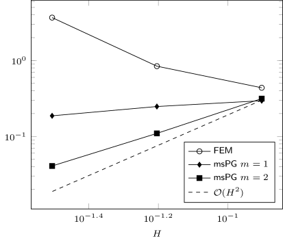
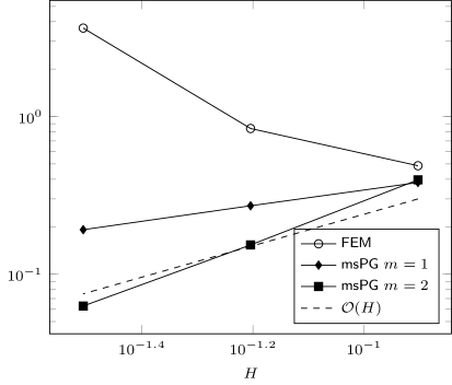
Fig. 1: Normalized errors $\|\cdot\|_{L^{2}(\Omega)}/\|u\|_{L^{2}(\Omega)}$ (left) and $\|\cdot\|_{V}/\|u\|_{V}$ (right) for the 3D example for $k=16$.

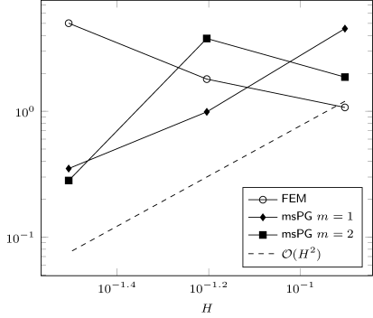
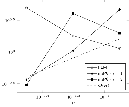
Fig. 2: Normalized errors $\|\cdot\|_{L^{2}(\Omega)}/\|u\|_{L^{2}(\Omega)}$ (left) and $\|\cdot\|_{V}/\|u\|_{V}$ (right) for the 3D example for $k=32$.

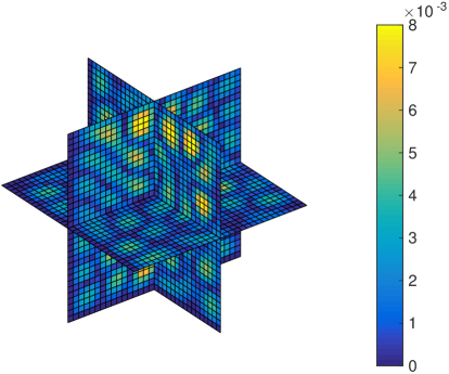
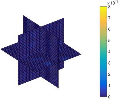
Fig. 3: Slice plots of the modulus of the pointwise error of the FEM (left) and the msPG method with $m=2$ (right) for the 3D example with $k=32$.

3.6 Numerical Experiment in 2D

We consider the square with hole $\Omega=(0,1)^{2}\setminus[0.375,0.625]^{2}$ with Robin boundary conditions $\Gamma_{R}=\partial(0,1)^{2}$ on the outer boundary and zero Dirichlet conditions $\Gamma_{D}=\partial[0.375,0.625]^{2}$ on the inner boundary. The Robin data is $g=0$ while $f$ is the approximate point source with components

$$f_{j}(x)=\begin{cases}\exp\left(-\frac{1}{1-(20|x|)^{2}}\right)&\text{for }|x|<1/20\\ 0&\text{else}\end{cases}\qquad j=1,2.$$

The Lamé parameters are $\mu=1=\lambda$. The coarse meshes $\mathcal{T}_{H}$ have mesh sizes $H=2^{-5},2^{-6},2^{-7},2^{-8}$ and the reference mesh size is $h=2^{-11}$. Since the exact solution is unknown, we took the finite element solution with respect to the fine-scale mesh $\mathcal{T}_{h}$ as a reference solution. We chose wavenumbers $k=64$ and $k=128$. Figure 4 displays the normalized errors in the $\|\cdot\|_{L^{2}(\Omega)}$ norm and the $\|\cdot\|_{V}$ norm for $k=64$ for the FEM and the msPG method with $m=1$ and $m=2$. The errors for $k=128$ are shown in Figure 5. Figure 6 shows the elastic displacement computed with the msPG method for $m=2$ and $H=2^{-7}$. In all cases, the msPG approximation has optimal order under the natural resolution condition whereas the FEM suffers from pollution.

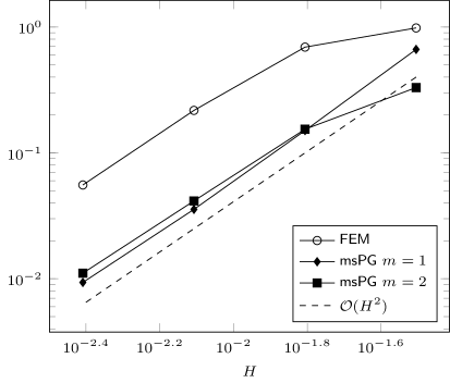
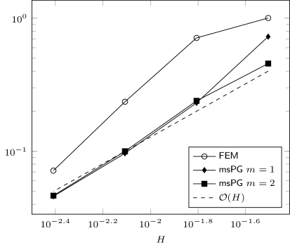
Fig. 4: Normalized errors $\|\cdot\|_{L^{2}(\Omega)}/\|u\|_{L^{2}(\Omega)}$ (left) and $\|\cdot\|_{V}/\|u\|_{V}$ (right) for the 2D example for $k=64$.

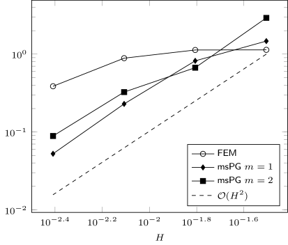
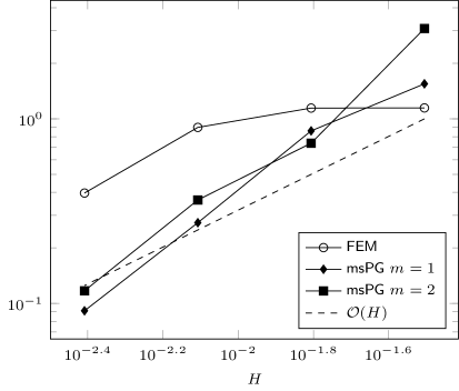
Fig. 5: Normalized errors $\|\cdot\|_{L^{2}(\Omega)}/\|u\|_{L^{2}(\Omega)}$ (left) and $\|\cdot\|_{V}/\|u\|_{V}$ (right) for the 2D example for $k=128$.

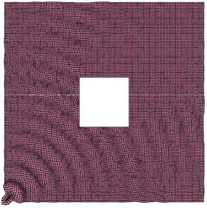
Fig. 6: Elastic displacement in the 2D experiment for $k=128$ computed with the msPG method with $m=2$ and $H=2^{-7}$; amplified by a factor 900.

Appendix A Newton Potential Estimates

In this appendix, we will estimate the Newton potential (2.11). We utilize Fourier techniques as in [37], to calculate the $k$-bounds on $N_{k}$. The main result is the following.

Theorem A.1.

Let $f\in(L^{2}({\Omega}))^{3},$ for the Newton potential (2.11) we have the estimate

$$k^{-1}{\left\lVert N_{k}(f)\right\rVert}_{H^{2}({\Omega})}+{\left\lVert N_{k}(f)\right\rVert}_{H^{1}({\Omega})}+k{\left\lVert N_{k}(f)\right\rVert}_{L^{2}({\Omega})}\leq C{\left\lVert f\right\rVert}_{L^{2}({\Omega})},$$ (A.1)

where $C>0$ is independent of $k$ and depends only on $\Omega,\mu,\lambda$.

• According to the representation (2.10) the Newton potential can be split as $N_{k}(f)=N_{k}^{E}(f)+N_{k}^{H}(f)$ where

  $$N_{k}^{E}(f)(x)=\int_{\Omega}G_{k}^{E}(x-y)f(y)dy\quad\text{and}\quad N_{k}^{H}(f)(x)=\int_{\Omega}G_{k}^{H}(x-y)f(y)dy.$$

  The second part $N_{k}^{H}(f)$ is a vector version of the Newton potential of the acoustic Helmholtz equation, for which the bounds $k^{1-m}\|N_{k}^{H}(f)\|_{H^{m}(\Omega)}\leq C\|f\|_{L^{2}(\Omega)}$ for $m=0,1,2$ have been established in [37]. We therefore only need to prove $k^{1-m}\|N_{k}^{E}(f)\|_{H^{m}(\Omega)}\leq C\|f\|_{L^{2}(\Omega)}$, $m=0,1,2$, for the elastic part of the Newton potential.

  We start by defining the auxiliary potential

  $$\widetilde{N}_{k}^{E}(f)(x)=\int_{\Omega}\widetilde{G}_{k}^{E}(x-y)f(y)dy\qquad\text{where}\quad\widetilde{G}_{k}^{E}(r)=\frac{1}{k^{2}}\left(\frac{e^{\mathbf{i}k_{2}r}}{r}-\frac{e^{\mathbf{i}k_{1}r}}{r}\right)$$ (A.2)

  and observe from the representation (2.10b) that

  $$|N_{k}^{E}(f)|_{H^{m}(\Omega)}\leq C|\widetilde{N}_{k}^{E}(f)|_{H^{m+2}(\Omega)}.$$

  The simplification in working with $\widetilde{G}_{k}^{E}$ is that, in contrast to $G_{k}^{E}$, it only depends on the radial component. We proceed with a cut-off function argument and using Fourier techniques as in [35]. Suppose ${\Omega}\subset B_{R}(0)$ for some $R>0$. We extend $f$ to zero when considered outside of ${\Omega}$ into $B_{R}$, but do not relabel. We define the cutoff function $\eta\in C^{\infty}(\mathbb{R}_{\geq 0})$, such that $\operatorname{supp}(\eta)\subset[0,4R]$

  $$\forall x\in\mathbb{R}_{\geq 0}:\quad 0\leq\eta(x)\leq 1,\quad|\eta^{\prime}(x)|\leq C/R,\quad\eta|_{[0,2R]}=1,\quad\eta|_{[4R,\infty)}=0.$$

  We set $M(x):=\eta(|x|)$ and define an augmented Newton potential of (A.2) as

  $$v^{\eta}(x)=\int_{B_{R}(0)}M(x-y)\widetilde{G}_{{k}}^{E}(x-y)f(y)dy\quad\text{for }x\in\mathbb{R}^{3},$$ (A.3)

  where $\widetilde{G}_{k}^{E}$ is given by (A.2). For functions $u$ with compact support, recall the Fourier transform and the inverse transform are given for $x,\xi\in\mathbb{R}^{3}$ by

  $$\hat{u}(\xi)=\frac{1}{(2\pi)^{3/2}}\int_{\mathbb{R}^{3}}e^{-\mathbf{i}x\cdot\xi}u(x)dx\quad\text{ and }\quad{u}(x)=\frac{1}{(2\pi)^{3/2}}\int_{\mathbb{R}^{3}}e^{\mathbf{i}x\cdot\xi}\hat{u}(\xi)d\xi.$$

  For $f$ has support in $B_{R}$ we write the truncated Newton potential component-wise, using the Einstein summation convention, as $v_{i}^{\eta}(x)=((M\widetilde{G}_{k}^{E})_{ij}*f_{j})(x)$, for $i,j=1,2,3$. Taking the Fourier transform, using the standard convolution identity, we obtain $\hat{v}_{i}^{\eta}(\xi)=(2\pi)^{3/2}(\widehat{(M\widetilde{G}_{k}^{E})}_{ij}\hat{f}_{j})(\xi)$, for $i,j=1,2,3$. For a multi-index $\alpha\in\mathbb{N}_{0}^{3}$, (non-negative integer vectors of dimension 3), we denote the corresponding multi-index derivatives as $\partial^{\alpha}$ in the standard way. For the corresponding to the derivatives in the Fourier variable, we denote the function $P_{\alpha}:\mathbb{R}^{3}\to\mathbb{R}^{3}$, $P_{\alpha}(\xi)=\xi^{\alpha}$. For $2\leq|\alpha|\leq 4$, we see using the Plancherel identity that

  $${\left\lVert\partial^{\alpha}v_{i}^{\eta}\right\rVert}_{L^{2}(\mathbb{R}^{3})} ={\left\lVert P_{\alpha}\hat{v}_{i}^{\eta}\right\rVert}_{L^{2}(\mathbb{R}^{3})}=(2\pi)^{3/2}{\left\lVert P_{\alpha}\widehat{(M\widetilde{G}_{k}^{E})}_{ij}\hat{f}_{j}\right\rVert}_{L^{2}(\mathbb{R}^{3})}$$

  $$\leq(2\pi)^{3/2}\sup_{\xi\in\mathbb{R}^{3}}\left|P_{\alpha}(\xi)\widehat{(M\widetilde{G}_{k}^{E})}_{ij}(\xi)\right|{\left\lVert\hat{f}_{j}\right\rVert}_{L^{2}(\mathbb{R}^{3})}.$$

  Thus, our estimate relies on the estimation of the supremum over $\xi$ on the last term. This will be estimated in Lemma A.2 below, where we prove that

  $$\sup_{\xi\in\mathbb{R}^{3}}\left|P_{\alpha}(\xi)\widehat{(M\widetilde{G}_{k}^{E})}_{ij}(\xi)\right|\leq Ck^{|\alpha|-3}.$$

  This implies the asserted estimate. ∎

We now state and prove our main technical lemma used in the proof of Theorem 2.3.

Lemma A.2.

Let $(\widetilde{G}_{k}^{E})_{ij}$ be given by (A.2) and $M$ a cutoff function as above. Then, there exists a $C>0$ depending only on $R,\mu,\lambda$ and not on $k$, so that for $|\alpha|=2,3,4$,

$$\sup_{\xi\in\mathbb{R}^{3}}\left|P_{\alpha}(\xi)\widehat{(M\widetilde{G}_{k}^{E})}_{ij}(\xi)\right|\leq Ck^{|\alpha|-3},$$

for $i,j=1,2,3$.

• We proceed as in [37, Lemma 3.7]. Since $G_{k}^{E}$ from (A.2) depends only on the radial component we can write

  $$\widetilde{G}_{k}^{E}(r)=g_{k}(r):=\frac{1}{k^{2}}\left(\frac{e^{\mathbf{i}k_{2}r}}{r}-\frac{e^{\mathbf{i}k_{1}r}}{r}\right)\quad\text{where }r=|x|.$$ (A.4)

  A key observation is that $\widetilde{G}_{k}^{E}(r)\to 0$ as $r\to 0$, which corresponds to the boundary terms of the following integration by parts vanishing, allowing for higher order derivative estimates. We then have from the definition of the Fourier transform and a change of variables to spherical coordinates

  $$\widehat{M\widetilde{G}_{k}^{E}}(\xi)=\frac{1}{(2\pi)^{3/2}}\int_{\mathbb{R}^{3}}e^{-\mathbf{i}x\cdot\xi}M(x)\widetilde{G}_{k}^{E}(x)dx=\frac{1}{(2\pi)^{3/2}}\int_{0}^{\infty}\eta(r)g_{k}(r)r^{2}\left(\int_{S^{2}}e^{-\mathbf{i}\zeta\cdot\xi}ds_{\zeta}\right)dr$$

  where $S^{2}$ is the unit sphere in $\mathbb{R}^{3}$. The inner integral was explicitly computed in [37, equation $($3.34$)$] and equals $4\pi\sin(r|\xi|)/(r|\xi|)$. We thus obtain

  $$\widehat{M\widetilde{G}_{k}^{E}}(\xi)=\frac{4\pi}{(2\pi)^{3/2}}\iota(|\xi|)\quad\text{with }\iota(s):=\int_{0}^{\infty}\eta(r)g_{k}(r)r^{2}\frac{\sin(rs)}{rs}dr.$$

  We closely follow the arguments of [37, Lemma 3.7] and estimate $s^{m}\iota(s)$ for $m=2,3,4$. For $m=2$ we use the representation (A.4) and integration by parts and compute

  $$|s^{2}\iota(s)| =k^{-2}\left|\int_{0}^{\infty}\eta(r)(e^{\mathbf{i}k_{2}r}-e^{\mathbf{i}k_{1}r})s\sin(rs)dr\right|=k^{-2}\left|\int_{0}^{\infty}\eta(r)(e^{\mathbf{i}k_{2}r}-e^{\mathbf{i}k_{1}r})\partial_{r}\cos(rs)dr\right|$$

  $$=k^{-2}\left|\int_{0}^{\infty}\partial_{r}\Big{(}\eta(r)(e^{\mathbf{i}k_{2}r}-e^{\mathbf{i}k_{1}r})\Big{)}\cos(rs)dr\right|$$

  $$\leq k^{-2}\left|\int_{0}^{\infty}\eta^{\prime}(r)(e^{\mathbf{i}k_{2}r}-e^{\mathbf{i}k_{1}r})\cos(rs)dr\right|+k^{-2}\left|\int_{0}^{\infty}\eta(r)(k_{2}e^{\mathbf{i}k_{2}r}-k_{1}e^{\mathbf{i}k_{1}r})\cos(rs)dr\right|.$$

  By using the properties of $\eta$ and $\eta^{\prime}$, the first term can be bounded by $k^{-2}C$ and the second one by $k^{-1}CR$, so that $|s^{2}\iota(s)|\leq k^{-1}C$. For $m=3$, in a similar fashion we use integration by parts twice and obtain

  $$|s^{3}\iota(s)| =k^{-2}\left|\int_{0}^{\infty}\eta(r)(e^{\mathbf{i}k_{2}r}-e^{\mathbf{i}k_{1}r})s^{2}\sin(rs)dr\right|$$

  $$=k^{-2}\left|\int_{0}^{\infty}\eta(r)(e^{\mathbf{i}k_{2}r}-e^{\mathbf{i}k_{1}r})\partial^{2}_{r}\sin(rs)dr\right|$$

  $$=k^{-2}\left|\int_{0}^{\infty}\partial^{2}_{r}\Big{(}\eta(r)(e^{\mathbf{i}k_{2}r}-e^{\mathbf{i}k_{1}r})\Big{)}\sin(rs)dr\right|.$$

  With arguments analogous to above we see that this is bounded by a constant $C$. Finally, for $m=4$ we compute

  $$|s^{4}\iota(s)|=k^{-2}\left|\int_{0}^{\infty}\eta(r)(e^{\mathbf{i}k_{2}r}-e^{\mathbf{i}k_{1}r})\partial^{3}_{r}\cos(rs)dr\right|=k^{-2}\left|\int_{0}^{\infty}\partial^{3}_{r}\Big{(}\eta(r)(e^{\mathbf{i}k_{2}r}-e^{\mathbf{i}k_{1}r})\Big{)}\cos(rs)dr\right|$$

  and see that this is bounded by $Ck$.

  In summary, we have shown $|s^{m}\iota(s)|\leq Ck^{m-3}$. This implies for $2\leq|\alpha|\leq 4$ that

  $$\sup_{\xi\in\mathbb{R}^{3}}\left|P_{\alpha}(\xi)\widehat{(M\widetilde{G}_{k}^{E})}_{ij}(\xi)\right|\leq C\sup_{s\geq 0}|s^{|\alpha|}\iota(s)|\leq Ck^{|\alpha|-3},$$

  which is the desired bound. ∎

We thank two anonymous referees who helped to obtain a sharper-in-$k$ stability bound and who pointed us to a much more direct argument for proof of the stability result compared with a prior manuscript version of this paper.

D. Gallistl gratefully acknowledges financial support by the DFG through SFB 1173; by the Baden-Württemberg Stiftung through the project ``Mehrskalenmethoden für Wellenausbreitung in heterogenen Materialien und Metamaterialien''; and by the European Research Council trough project DAFNE, ID 891734.

Bibliography

- [1] M. Abramowitz and I. A. Stegun. Handbook of mathematical functions with formulas, graphs, and mathematical tables, volume 55 of National Bureau of Standards Applied Mathematics Series. Washington, D.C., 1964.
- [2] I. M. Babuska and S. A. Sauter. Is the pollution effect of the fem avoidable for the Helmholtz equation considering high wave numbers? SIAM Journal on Numerical Analysis, 34(6):2392–2423, 1997.
- [3] D. Baskin, E. A. Spence, and J. Wunsch. Sharp high-frequency estimates for the Helmholtz equation and applications to boundary integral equations. SIAM J. Math. Anal., 48(1):229–267, 2016.
- [4] T. Betcke, S. N. Chandler-Wilde, I. G. Graham, S. Langdon, and M. Lindner. Condition number estimates for combined potential integral operators in acoustics and their boundary element discretisation. Numerical Methods for Partial Differential Equations, 27(1):31–69, 2011.
- [5] D. Brown, D. Gallistl, and D. Peterseim. Multiscale Petrov-Galerkin method for high-frequency heterogeneous Helmholtz equations. In M. Griebel and M. A. Schweitzer, editors, Meshfree Methods for Partial Differential Equations VII, volume 115 of Lect. Notes Comput. Sci. Eng., pages 85–115. Springer, Cham, 2017.
- [6] D. Brown and D. Peterseim. A multiscale method for porous microstructures. SIAM MMS, 14(3):1123–1152, 2016.
- [7] S. N. Chandler-Wilde, I. G. Graham, S. Langdon, and M. Lindner. Condition number estimates for combined potential boundary integral operators in acoustic scattering. Journal of Integral Equations and Applications, 21(2):229–279, 2009.
- [8] S. N. Chandler-Wilde, I. G. Graham, S. Langdon, and E. A. Spence. Numerical-asymptotic boundary integral methods in high-frequency acoustic scattering. Acta Numerica, 21:89–305, 2012.
- [9] S. N. Chandler-Wilde and P. Monk. Wave-number-explicit bounds in time-harmonic scattering. SIAM J. Math. Anal., 39(5):1428–1455, 2008.
- [10] T. Chaumont-Frelet and S. Nicaise. Wavenumber explicit convergence analysis for finite element discretizations of general wave propagation problem. HAL Preprint, hal-01685388. https://hal.inria.fr/hal-01685388.
- [11] E. U. Condon and G. H. Shortley. The Theory of Atomic Spectra. Cambridge University Press, 1951.
- [12] P. Cummings and X. Feng. Sharp regularity coefficient estimates for complex-valued acoustic and elastic Helmholtz equations. Mathematical Models and Methods in Applied Sciences, 16(01):139–160, 2006.
- [13] B. E. J. Dahlberg, C. E. Kenig, and G. C. Verchota. Boundary value problems for the systems of elastostatics in Lipschitz domains. Duke Math. J., 57(3):795–818, 12 1988.
- [14] A. R. Edmonds. Angular momentum in quantum mechanics, volume 4 of Investigations in physics. Princeton University Press, Princeton, 1957.
- [15] S. Esterhazy and J. Melenk. On stability of discretizations of the Helmholtz equation. In I. G. Graham, T. Y. Hou, O. Lakkis, and R. Scheichl, editors, Numerical Analysis of Multiscale Problems, volume 83 of Lect. Notes Comput. Sci. Eng., pages 285–324. Springer Berlin Heidelberg, 2012.
- [16] X. Feng and D. Sheen. An elliptic regularity coefficient estimate for a problem arising from a frequency domain treatment of waves. Trans. Amer. Math. Soc., 346(2):475–487, 1994.
- [17] X. Feng and H. Wu. Discontinuous Galerkin methods for the Helmholtz equation with large wave number. SIAM Journal on Numerical Analysis, 47(4):2872–2896, 2009.
- [18] X. Feng and H. Wu. -discontinuous Galerkin methods for the Helmholtz equation with large wave number. Mathematics of Computation, 80(276):1997–2024, 2011.
- [19] D. Gallistl and D. Peterseim. Stable multiscale Petrov-Galerkin finite element method for high frequency acoustic scattering. Comput. Methods Appl. Mech. Eng., 295:1–17, 2015.
- [20] P. Henning, A. Målqvist, and D. Peterseim. A localized orthogonal decomposition method for semi-linear elliptic problems. ESAIM Math. Model. Numer. Anal., 48(5):1331–1349, 2014.
- [21] P. Henning, A. Målqvist, and D. Peterseim. Two-level discretization techniques for ground state computations of Bose-Einstein condensates. SIAM J. Numer. Anal., 52(4):1525–1550, 2014.
- [22] P. Henning, P. Morgenstern, and D. Peterseim. Multiscale partition of unity. In M. Griebel and M. A. Schweitzer, editors, Meshfree Methods for Partial Differential Equations VII, volume 100 of Lect. Notes Comput. Sci. Eng. Springer, 2014.
- [23] P. Henning and D. Peterseim. Oversampling for the Multiscale Finite Element Method. Multiscale Model. Simul., 11(4):1149–1175, 2013.
- [24] U. Hetmaniuk. Fictitious domain decomposition methods for a class of partially axisymmetric problems: Application to the scattering of acoustic waves. PhD thesis, University of Colorado, 2002.
- [25] U. Hetmaniuk. Stability estimates for a class of Helmholtz problems. Commun. Math. Sci., 5(3):665–678, 2007.
- [26] G. C. Hsiao, R. E. Kleinman, and G. F. Roach. Weak solutions of fluid–solid interaction problems. Mathematische Nachrichten, 218(1):139–163, 2000.
- [27] C. E. Kenig. Boundary value problems of linear elastostatics and hydrostatics on Lipschitz domains. In Goulaouic-Meyer-Schwartz seminar, 1983–1984, pages Exp. No. 21, 13. École Polytech., Palaiseau, 1984.
- [28] M. Kitahara. Boundary Integral Equation Methods in Eigenvalue Problems of Elastodynamics and Thin Plates, volume 10 of Studies in Applied Mechanics. Elsevier Scientific Publishing Co., Amsterdam, 1985.
- [29] V. D. Kupradze. Potential methods in the theory of elasticity. Translated from the Russian by H. Gutfreund. Translation edited by I. Meroz. Israel Program for Scientific Translations, Jerusalem; Daniel Davey & Co., Inc., New York, 1965.
- [30] V. D. Kupradze. Three-dimensional problems of elasticity and thermoelasticity. North-Holland Series in Applied Mathematics and Mechanics. Elsevier, Burlington, 2012.
- [31] A. Målqvist and A. Persson. Multiscale techniques for parabolic equations. Numer. Math., 138(1):191–217, 2018.
- [32] A. Målqvist and D. Peterseim. Localization of elliptic multiscale problems. Math. Comp., 83(290):2583–2603, 2014.
- [33] W. McLean. Strongly Elliptic Systems and Boundary Integral Equations. Cambridge University Press, Cambridge, 2000.
- [34] J. M. Melenk. On generalized finite-element methods. PhD thesis, University of Maryland, College Park, 1995.
- [35] J. M. Melenk. Mapping properties of combined field Helmholtz boundary integral operators. SIAM Journal on Mathematical Analysis, 44(4):2599–2636, 2012.
- [36] J. M. Melenk and S. Sauter. Wavenumber explicit convergence analysis for Galerkin discretizations of the Helmholtz equation. SIAM Journal on Numerical Analysis, 49(3):1210–1243, 2011.
- [37] J. M. Melenk and S. A. Sauter. Convergence analysis for finite element discretizations of the Helmholtz equation with Dirichlet-to-Neumann boundary conditions. Math. Comp., 79(272):1871–1914, 2010.
- [38] C. S. Morawetz. Decay for solutions of the exterior problem for the wave equation. Comm. Pure Appl. Math., 28:229–264, 1975.
- [39] C. S. Morawetz and D. Ludwig. An inequality for the reduced wave operator and the justification of geometrical optics. Comm. Pure Appl. Math., 21:187–203, 1968.
- [40] J.-C. Nédélec. Acoustic and Electromagnetic Equations: Integral Representations for Harmonic Problems, volume 144 of Applied Mathematical Sciences. Springer-Verlag, New York, 2001.
- [41] D. Peterseim. Variational multiscale stabilization and the exponential decay of fine-scale correctors. In G. R. Barrenechea, F. Brezzi, A. Cangiani, and E. H. Georgoulis, editors, Building Bridges: Connections and Challenges in Modern Approaches to Numerical Partial Differential Equations, volume 114 of Lect. Notes Comput. Sci. Eng., pages 343–369. Springer, 2016.
- [42] D. Peterseim. Eliminating the pollution effect in Helmholtz problems by local subscale correction. Math. Comp., 86:1005–1036, 2017.
- [43] S. A. Sauter. A refined finite element convergence theory for highly indefinite Helmholtz problems. Computing, 78(2):101–115, 2006.
- [44] E. A. Spence. Wavenumber-explicit bounds in time-harmonic acoustic scattering. SIAM J. Math. Anal., 46(4):2987–3024, 2014.
- [45] R. Tezaur and C. Farhat. Three-dimensional discontinuous Galerkin elements with plane waves and lagrange multipliers for the solution of mid-frequency Helmholtz problems. International Journal for Numerical Methods in Engineering, 66(5):796–815, 2006.
- [46] B. Vainberg. On the short wave asymptotic behaviour of solutions of stationary problems and the asymptotic behaviour as of solutions of non-stationary problems. Russ. Math. Surv., 30(2):1–58, 1975.
- [47] C.-Y. Wang and J. D. Achenbach. Three-dimensional time-harmonic elastodynamic Green’s functions for anisotropic solids. Proceedings of the Royal Society of London A: Mathematical, Physical and Engineering Sciences, 449(1937):441–458, 1995.
- [48] J. Zitelli, I. Muga, L. Demkowicz, J. Gopalakrishnan, D. Pardo, and V. M. Calo. A class of discontinuous Petrov–Galerkin methods. Part IV: The optimal test norm and time-harmonic wave propagation in 1D. Journal of Computational Physics, 230(7):2406–2432, 2011.