Bayesian Community Detection

Abstract

We introduce a Bayesian estimator of the underlying class structure in the stochastic block model, when the number of classes is known. The estimator is the posterior mode corresponding to a Dirichlet prior on the class proportions, a generalized Bernoulli prior on the class labels, and a beta prior on the edge probabilities. We show that this estimator is strongly consistent when the expected degree is at least of order $\log^{2}{n}$, where $n$ is the number of nodes in the network.

and

t1Research supported by Netherlands Organization for Scientific Research NWO. t2The research leading to these results has received funding from the European Research Council under ERC Grant Agreement 320637.

1 Introduction

The stochastic block model (SBM) (Holland, Laskey and Leinhardt, 1983) is a model for network data in which individual nodes are considered members of classes or communities, and the probability of a connection occurring between two individuals depends solely on their class membership. It has been applied to social, biological and communication networks, for example in Park and Bader (2012), Bickel and Chen (2009) and Snijders and Nowicki (1997) amongst many others. There are many extensions of the SBM for various applications, including the degree-corrected SBM (Karrer and Newman, 2011; Zhao, Levina and Zhu, 2012) which accounts for possible heterogeneity among nodes within the same class, and the mixed-membership SBM (Airoldi et al., 2008), in which the assumption that the classes are disjoint is removed. These extensions allow for additional modelling flexibility.

Two main SBM research directions are the recovery of the class labels (community detection) and recovery of the remaining model parameters, consisting of the probability vector generating the class labels, and the class-dependent probabilities of creating an edge between nodes. In this paper, we focus on community detection, noting that once strong consistency of a community detection method has been established, consistency of the natural plug-in estimators for the remaining parameters follows directly by results in (Channarond, Daudin and Robin, 2012).

A large number of methods for recovering the class labels has been proposed. Those most closely related to this work are the modularities. Newman and Girvan (2004) introduced the term modularity for ‘a measure of the quality of a particular division of a network’. They described one such measure for models in which edges are more likely to occur within classes than between classes, in which case there is a community structure in the colloquial sense, although the SBM does not require this assumption. Bickel and Chen (2009) studied more general modularities, defining them as functions of the number of connections between all combinations of classes and the proportion of nodes placed in each class. They introduced the likelihood modularity, and provided general conditions under which modularities are consistent. Their method and theory was extended to the degree-corrected SBM by Zhao, Levina and Zhu (2012).

Spectral methods for community detection have gained in popularity, and refined results on error bounds are now available for the SBM and extensions of the SBM, as evidenced in Rohe, Chatterjee and Yu (2011), Jin (2015), Sarkar and Bickel (2015) and Lei and Rinaldo (2015) for example. Many other algorithms have been introduced, most of them currently lacking formal proofs of consistency. A notable exception is the Largest Gaps algorithm (Channarond, Daudin and Robin, 2012), which only takes the degree of each node as its input, and is strongly consistent under a separability condition.

A Bayesian approach towards recovering the class assignments in the SBM was first suggested by Snijders and Nowicki (1997), motivated by computational advantages of Gibbs sampling over maximum likelihood estimation. They considered two classes and proposed uniform priors on the class proportions and the edge probabilities. This approach was extended in (Nowicki and Snijders, 2001) to allow for more classes, with a Dirichlet prior on the class proportions and beta priors on the edge probabilities. Hofman and Wiggins (2008) described a similar Bayesian approach for a special case of the SBM and suggested a variational approach to overcome the computational issues associated with maximizing over all possible class assignments.

Bayesian methods for the SBM have barely been studied from a theoretical point of view, although recent results for parameter recovery by Pati and Bhattacharya (2015), for detecting the number of communites by Hayashi, Konishi and Kawamoto (2016) and for an empirical Bayes approach to community detection by Suwan et al. (2016) are encouraging. In this work, we provide theoretical results on community detection, establishing that the Bayesian posterior mode is strongly consistent for the class labels if the expected degree is at least of order $\log^{2}{n}$, where $n$ is the number of nodes. This is proven by relating the posterior mode to the maximizer of the likelihood modularity of Bickel and Chen (2009). The likelihood modularity has been claimed to be strongly consistent under the weaker assumption that the expected degree is of larger order than $\log{n}$ (Bickel and Chen, 2009; Zhao, Levina and Zhu, 2012; Bickel et al., 2015). However, their proof assumes that the likelihood modularity is globally Lipschitz, while it is only locally so. The Bayesian method is based on a combination of likelihood and prior, and for this reason the proof of our main theorem, Theorem 3.2, runs into a similar problem. We were able to resolve this only under the slightly stronger assumption that the expected degree is of larger order than $(\log{n})^{2}$. The literature on other methods for community detection shows that the order $\log n$ is sufficient for consistent detection. However, these results are usually obtained under additional assumptions such as a restriction to two classes or an ordering of the connection probabilities, and their implications for the likelihood or Bayesian modularities is unclear. We discuss this and the relevant literature further following the statement of our main result in Section 3.5.

This paper is organized as follows. We introduce the SBM and the associated notation in Section 2. Our main results are in Section 3, where we describe the prior and the link with the likelihood modularity, present the consistency results and discuss the underlying assumptions, especially those on the expected degree. The method is illustrated on a data set in Section 4, and we conclude with a Discussion in Section 5. All proofs are given in the Appendix.

2 The Stochastic Block Model

We introduce the notation and generative model for the SBM with $K\in\{1,2,\ldots\}$ classes. Consider an undirected random graph with $n$ nodes, numbered $1,2,\ldots,n$, and edges encoded by the $n\times n$ symmetric adjacency matrix $(A_{ij})$, with entries in $\{0,1\}$. Thus $A_{ij}=A_{ji}$ is equal to 1 or 0 if the nodes $i$ and $j$ are or are not connected by an edge, respectively. Self-loops are not allowed, so $A_{ii}=0$ for $i=1,\ldots,n$. The generative model for the random graph is:

1. The nodes are randomly labeled with i.i.d. variables $Z_{1},\ldots,Z_{n}$, taking values in a finite set $\{1,...,K\}$, according to probabilities $\pi=(\pi_{1},\ldots,\pi_{K})$.

2. Given $Z=(Z_{1},\ldots,Z_{n})$, the edges are independently generated as Bernoulli variables with $\mathbb{P}(A_{ij}=1\mid Z)=P_{Z_{i},Z_{j}}$, for $i<j$, for a given $K\times K$ symmetric matrix $P=(P_{ab})$.

The probability vector $\pi$ is considered fixed, but unknown. Although this is not visible in the notation, the matrix $P$ may change with $n$, a case of particular interest being that $P$ tends to zero, which gives a sparse graph. The order of magnitude of $\|P\|_{\infty}=\max_{a,b}P_{ab}$ is the same as the order of magnitude of $\rho_{n}=\sum_{a,b}\pi_{a}\pi_{b}P_{ab}$, the probability of there being an edge between two randomly selected nodes. The expected degree of a randomly selected node is $\lambda_{n}=(n-1)\rho_{n}$, and twice the expected total number of edges in the network is $\mu_{n}=n(n-1)\rho_{n}$.

The likelihood for the model is given by

$$\prod_{i<j}P_{Z_{i}Z_{j}}^{A_{ij}}(1-P_{Z_{i}Z_{j}})^{1-A_{ij}}\prod_{i}\pi_{Z_{i}}=\prod_{a\leq b}P_{ab}^{O_{ab}(Z)}(1-P_{ab})^{n_{ab}(Z)-O_{ab}(Z)}\prod_{a}\pi_{a}^{n_{a}(Z)},$$ (1)

where $O_{ab}(Z)$ is the number of edges between nodes labelled $a$ and $b$ by the labelling $Z$, $n_{ab}(Z)$ is the maximum number of edges that can be created between nodes labelled $a$ and $b$, and $n_{a}(Z)$ is the number of nodes labelled $a$, and $a$ and $b$ range over $\{1,2,\ldots,K\}$.

More formally, for a given labelling $e=(e_{1},\ldots,e_{n})\in\{1,\ldots,K\}^{n}$ of nodes, and class labels $a,b\in\{1,\ldots,K\}$, we define

$$O_{ab}(e) =\begin{cases}\sum_{i,j}A_{ij}\textbf{1}_{\{e_{i}=a,e_{j}=b\}},&a\neq b,\\ \sum_{i<j}A_{ij}\textbf{1}_{\{e_{i}=a,e_{j}=b\}},&a=b,\end{cases}$$

$$n_{ab}(e) =\begin{cases}n_{a}(e)n_{b}(e),&a\neq b,\\ \tfrac{1}{2}n_{a}(e)(n_{a}(e)-1),&a=b,\end{cases}$$

$$n_{a}(e) =\sum_{i=1}^{n}\textbf{1}_{\{e_{i}=a\}}.$$

Since the matrix $A$ is symmetric with zero diagonal by assumption, for $a\not=b$ the variable $O_{ab}(e)$ can also be written as $\sum_{i<j}A_{ij}[\textbf{1}_{\{e_{i}=a,e_{j}=b\}}+\textbf{1}_{\{e_{j}=a,e_{i}=b\}}]$, which explains the different appearances of the diagonal and off-diagonal entries. The numbers $n_{ab}(e)$ are equal to the numbers $O_{ab}(e)$ when all $A_{ij}$ are equal to 1. We collect the variables $O_{ab}(e)$ and $n_{ab}(e)$ in $K\times K$ matrices $O(e)$ and $n(e)$.

Now consider the $K\times K$ probability matrix $R(e,c)$ and $K$ probability vector $f(e)$ with entries

$$R_{ab}(e,c)=\frac{1}{n}\sum_{i=1}^{n}\textbf{1}_{\{e_{i}=a,c_{i}=b\}},\qquad\quad f_{a}(e)=\frac{n_{a}(e)}{n}.$$ (2)

The row sums of $R(e,c)$ are equal to $R(e,c)\textbf{1}=f(e)$, while the column sums are equal to $\textbf{1}^{T}R(e,c)=f(c)^{T}$. Thus, the matrix $R(e,c)$ can be seen as a coupling of the marginal probability vectors $f(e)$ and $f(c)$. If $e=c$, then it is diagonal with diagonal $f(c)=f(e)$. More generally, the matrix can be viewed as measuring the discrepancy between labellings $e$ and $c$. This can be precisely measured as half the $L_{1}$-distance of $R(e,c)$ to its diagonal, as evidenced by Lemma 2.1, which is noted in Bickel and Chen (2009).

For a vector $v$ we denote by ${\rm Diag}(v)$ the diagonal matrix with diagonal $v$, and for a matrix $M$ we denote its diagonal by $\mathop{\rm diag\,}\nolimits(M)$.

Lemma 2.1.

For every labelling $c,e$ in the $K$-class stochastic block model:

$$\frac{1}{n}\sum_{i=1}^{n}\textbf{1}_{\{c_{i}\neq e_{i}\}}=\tfrac{1}{2}\|{\rm Diag}(f(c))-R(e,c)\|_{1}.$$

Proof.

The diagonal of $R(e,c)$ gives the fractions of labels on which $c$ and $e$ agree. Hence the left side of the lemma is $1-\sum_{a}R_{aa}(e,c)=\sum_{a}(f_{a}(c)-R_{aa}(c))$ . The elements of both $K\times K$ matrices ${\rm Diag}(f(c))$ and $R(e,c)$ can be viewed as probabilities that add up to 1. Thus the sum of the differences of the diagonal elements is minus the sum of the differences of the off-diagonal elements. Because $f_{a}(c)\geq R_{aa}(e,c)$ for every $a$, we have $\sum_{a}(f_{a}(c)-R_{aa}(e,c))=\sum_{a}|f_{a}(c)-R_{aa}(e,c)|$. Similarly the off-diagonal elements of ${\rm Diag}(f(c))$, which are zero, are smaller than the off-diagonal elements of $R(e,c)$ and hence we can add absolute values. Thus the sum over the diagonal is half the sum of the absolute values of all terms in ${\rm Diag}(f(c))-R(e,c)$. ∎

3 Bayesian Approach to Community Detection

Our main results are presented in this section. We first discuss the choice of prior in Section 3.1, and define the estimator, in Section 3.2. The resulting Bayesian modularity is closely related to the likelihood modularity of Bickel and Chen (2009). The relationship is clarified in Section 3.3. We briefly consider the issue of identifiability in the SBM in Section 3.4, and conclude with our main theorem on the strong consistency of the Bayesian modularity in Section 3.5.

3.1 The prior

We adopt the Bayesian approach of Nowicki and Snijders (2001). We put prior distributions on the parameters of the stochastic block model with $K$ known, the vector $\pi$ and the matrix $P$, yielding a joint probability distribution of $(A,Z,\pi,P)$. Next we marginalize over $\pi$ and $P$ as in McDaid et al. (2013), leading to a joint distribution of $(A,Z)$. Finally we “estimate” the unobserved vector $Z$ by the posterior mode of the conditional distribution of $Z$ given $A$. From a frequentist point of view this means that $Z$ is treated as a parameter of the problem, equipped with a hierarchical prior that chooses first $\pi$ and then $Z$. Accordingly we shall change notation from $Z$ to $e$, reserving $Z$ for the frequentist description of the stochastic block model in Section 2.

The prior on $\pi$ is a Dirichlet, and independently the $P_{ab}$ for $a\leq b$ receive independent beta priors:

$$\pi \sim{\rm Dir}(\alpha,\ldots,\alpha),$$

$$P_{ab} \stackrel{{\scriptstyle i.i.d.}}{{\sim}}{\rm Beta}(\beta_{1},\beta_{2}),\quad 1\leq a\leq b\leq K.$$

This is essentially the same set-up as in Nowicki and Snijders (2001) and McDaid et al. (2013), except that we use a more flexible ${\rm Beta}(\beta_{1},\beta_{2})$ instead of a uniform prior on the $P_{ab}$. We assume $\alpha,\beta_{1},\beta_{2}>0$.

We complete the Bayesian model by specifying class labels $e=(e_{1},\ldots,e_{n})$ and edges $A=(A_{ij}:i<j)$ through

$$e_{i}\mid\pi,P \stackrel{{\scriptstyle i.i.d.}}{{\sim}}\pi,\quad 1\leq i\leq n,$$

$$A_{ij}\mid\pi,P,e \stackrel{{\scriptstyle ind.}}{{\sim}}{\rm Bernoulli}(P_{e_{i},e_{j}}),\quad 1\leq i<j\leq n.$$

Abusing notation we write $p(e)$, $p(A\mid e)$ and $p(e\mid A)$ for marginal and conditional probability density functions.

3.2 The Bayesian modularity

The Bayesian estimator of the class labels will be the posterior mode, that is:

$$\widehat{e}=\mathop{\rm argmax}\limits_{e}p(e\mid A).$$

The posterior mode can be interpreted as a modularity-based estimator in the sense of Bickel and Chen (2009), in that it maximizes a function that only depends on the $O_{ab}(e)$ and the $n_{a}(e)$. This can be seen from the joint density of $(A,e)$, which is found by marginalizing the likelihood (1) over $\pi$ and $P$. The conjugacy between the multinomial and Dirichlet distributions gives the marginal density of the class assignment $e$ as:

$$p(e) =\int_{S_{K}}\prod_{a}\pi_{a}^{n_{a}(e)}\frac{\prod_{a}\pi_{a}^{\alpha-1}}{D(\alpha)}\,d\pi=\frac{\Gamma(\alpha K)}{\Gamma(\alpha)^{K}\Gamma(n+\alpha K)}\prod_{a}\Gamma(n_{a}(e)+\alpha).$$ (3)

Here the integral is relative to the Lebesgue measure on the $K$-dimensional unit simplex and $D(\alpha)=\Gamma(\alpha)^{K}/\Gamma(K\alpha)$ is the norming constant for the Dirichlet density. Similarly the conjugacy between the Bernoulli and Beta distributions gives the marginal conditional density of $A$ given $e$ as:

$$p(A\mid e) =\int_{[0,1]^{K(K+1)/2}}\prod_{a\leq b}P_{ab}^{O_{ab}(e)}(1-P_{ab})^{n_{ab}(e)-O_{ab}(e)}\prod_{a\leq b}\frac{P_{ab}^{\beta_{1}-1}(1-P_{ab})^{\beta_{2}-1}}{B(\beta_{1},\beta_{2})}\,dP$$

$$=\prod_{a\leq b}\frac{1}{B(\beta_{1},\beta_{2})}B(O_{ab}(e)+\beta_{1},n_{ab}(e)-O_{ab}(e)+\beta_{2}),$$ (4)

where $B(x,y)=\Gamma(x)\Gamma(y)/\Gamma(x+y)$ is the beta-function. The joint density of $A$ and $e$ is given by the product of (3) and (4), and $n^{-2}$ times its logarithm is up to a constant that is free of $e$ equal to

$$Q_{B}(e)=\frac{1}{n^{2}}\sum_{1\leq a\leq b\leq K}\log B(O_{ab}(e)+\beta_{1},n_{ab}(e)-O_{ab}(e)+\beta_{2})+\frac{1}{n^{2}}\sum_{a=1}^{K}\log\Gamma(n_{a}(e)+\alpha).$$

This is a modularity in the sense of Bickel and Chen (2009), which we define as the Bayesian modularity. As $p(e\mid A$) is proportional to $p(e,A)$, the posterior mode is equal to the class assignment that maximizes the Bayesian modularity, so the Bayesian estimator is equal to:

$$\widehat{e}=\mathop{\rm argmax}\limits_{e}Q_{B}(e).$$ (5)

3.3 Similarity to the likelihood modularity

The Bayesian modularity $Q_{B}(e)$ consists of a two parts, originating from the likelihood and the prior on the classification, respectively. The first part is close to the likelihood modularity given by

$$Q_{ML}(e)=\frac{1}{n^{2}}\sum_{1\leq a\leq b\leq K}n_{ab}(e)\,\tau\Bigl{(}\frac{O_{ab}(e)}{n_{ab}(e)}\Bigr{)},$$

where $\tau(x)=x\log{x}+(1-x)\log(1-x)$. This criterion, obtained in Bickel and Chen (2009), results from replacing in the log conditional likelihood of $A$ given $e$ (the logarithm of (1) with $Z$ replaced by $e$ and discarding the term involving the parameters $\pi_{a}$) the parameters $P_{ab}$ by their maximum likelihood estimators $\hat{P}_{ab}=O_{ab}(e)/n_{ab}(e)$. In other words, the parameters are profiled out rather than integrated out as for the Bayesian modularity. The corresponding estimator

$$\widehat{e}_{ML}=\mathop{\rm argmax}\limits_{e}Q_{ML}(e)$$

is consistent, and hence one may hope that the Bayesian estimator can be proved consistent by showing that the Bayesian and likelihood modularities are close. This will indeed be our line of approach, but the execution must be done with care. For instance, the second, prior part of the Bayesian modularity does play a role in the proof of strong consistency, although it is negligible when proving weak consistency.

The following lemma links the Bayesian and likelihood modularities.

Lemma 3.1.

There exists a constant $C$ such that, for ${\cal E}=\{1,\ldots,K\}^{n}$ the set of all possible labellings:

$$\max_{e\in{\cal E}}\Bigl{|}Q_{B}(e)-Q_{ML}(e)-Q_{P}(e)\Bigr{|}\leq\frac{C\log n}{n^{2}}.$$

for

$$Q_{P}(e)=\frac{1}{n^{2}}\sum_{a:n_{a}+\lfloor{\alpha}\rfloor\geq 2}n_{a}(e)\log(n_{a}(e))-\frac{1}{n}.$$

Consequently $\max_{e\in{\cal E}}\bigl{|}Q_{B}(e)-Q_{ML}(e)\bigr{|}={\cal O}\bigl{(}\log n/{n}\bigr{)}$.

3.4 Identifiability and consistency

A classification $\widehat{e}$ is said to be weakly consistent if the fraction of misclassified nodes tends to zero (partial recovery), and strongly consistent if the probability of misclassifying any of the nodes tends to zero (exact recovery). In defining consistency in a precise manner, the complication of the possible unidentifiability of the labels needs to be dealt with. From the observed data $A$ we can at best recover the partition of the $n$ nodes in the $K$ classes with equal labels $Z_{i}$, but not the values $Z_{1},\ldots,Z_{n}$ of the labels, in the set $\{1,2,\ldots,K\}$, attached to the classes. Thus consistency will be up to a permutation of labels.

To make this precise define, for a given permutation $(1,\ldots,K)\to\left(\sigma(1),\ldots,\sigma(K)\right)$, the permutation matrix $P_{\sigma}$ as the matrix with rows

$$e_{\sigma(1)}^{T}$$

$$\ \vdots$$

$$e_{\sigma(K)}^{T},$$

for $e_{1},\ldots,e_{K}$ the unit vectors in $\mathbb{R}^{K}$. Then pre-multiplication of a matrix by $P_{\sigma}$ permutes the rows, and post-multiplication by $P_{\sigma}^{T}$ the columns: $P_{\sigma}R$ is the matrix with $j$th row equal to the $\sigma(j)$th row of $R$, and $RP_{\sigma}^{T}$ is the matrix with $j$th column the $\sigma(j)$th column of $R$. Thus $P_{\sigma}R(e,Z)$ is the matrix that would result if we would permute the labels of the classes of the assignment $e$, and $P_{\sigma}PP_{\sigma}^{T}$ and $P_{\sigma}R(e,Z)P_{\sigma}^{T}$ are the matrices that would result if we would relabel the classes throughout. Since we cannot recover the labels, the matrix $P_{\sigma}R(e,Z)$ is just as good or bad as $R(e,Z)$ for measuring discrepancy between a labelling $e$ and the true labelling $Z$; furthermore, nothing should change if we choose different names for the classes.

Thus, taking into account the unidentifiability of the labels, by Lemma 2.1, an estimator $\widehat{e}$ is weakly consistent if

$$\|P_{\sigma}R(\widehat{e},Z)-{\rm Diag}(f(Z))\|_{1}\to 0,$$

for some permutation matrix $P_{\sigma}$. The classification $\widehat{e}$ is said to be strongly consistent if

$$\mathbb{P}(P_{\sigma}R(\widehat{e},Z)={\rm Diag}(f(Z)))\to 1,$$

for some permutation matrix $P_{\sigma}$.

The permutation matrix $P_{\sigma}$ is for large $n$ uniquely defined: if $\|({P_{\sigma}})_{j}R-{\rm Diag}(\pi)\|_{1}\leq\min_{a}\pi_{a}$, for $j=1,2$, then $(P_{\sigma})_{1}=(P_{\sigma})_{2}$. This follows because the assumption implies that $\|(P_{\sigma})_{1}^{-1}{\rm Diag}(\pi)-(P_{\sigma})_{2}^{-1}{\rm Diag}(\pi)\|_{1}\leq 2\min_{a}\pi_{a}$, by the triangle inequality and the fact that the $L_{1}$-norm is invariant under permutations. Furthermore, for $P_{\sigma}=(P_{\sigma})_{2}(P_{\sigma})_{1}^{-1}$ the left side is $\|P_{\sigma}{\rm Diag}(\pi)-{\rm Diag}(\pi)\|_{1}$, which is at least two times the sum of the two smallest coordinates of $\pi$ if $P_{\sigma}\not=I$.

A necessary requirement for consistency is that the classes can be recovered from the likelihood, i.e. the model parameters must be identifiable. If $\pi$ has strictly positive coordinates, so that all labels will appear in the data eventually, then as explained in Bickel and Chen (2009) an appropriate condition is that $P$ does not have two identical rows. If $\pi_{a}=0$ for some $a$, then class $a$ will never be consumed; the identifiability condition should then be imposed after deleting the $a$th column from $P$. Thus, we call the pair $(P,\pi)$ identifiable if the rows of $P$ are different after removing the columns corresponding to zero coordinates of $\pi$. Throughout we assume that $P$ is symmetric.

3.5 Consistency results and assumptions

We are now ready to present our results on consistency for the Bayesian maximum a posteriori (MAP) estimator (5). Theorem 3.2 shows strong consistency of the Bayesian estimator if $\lambda_{n}\gg(\log n)^{2}$. The proof rests on a proof of weak consistency under similar conditions, stated in the appendix as Theorem A.1.

Recall that $\rho_{n}=\sum_{a,b}\pi_{a}\pi_{b}P_{ab}$ is the probability of a new edge, and $\lambda_{n}=(n-1)\rho_{n}$ is the expected degree of a node.

Theorem 3.2 (strong consistency).

1. If $(P,\pi)$ is fixed and identifiable with $0<P<1$ and $\pi>0$ then the MAP classifier $\widehat{e}=\arg\max_{e}Q_{B}(e)$ is strongly consistent.

2. If $P=\rho_{n}S$, where $(S,\pi)$ is fixed and identifiable with $S>0$ and $\pi>0$, then the MAP classifier $\widehat{e}=\arg\max_{e}Q_{B}(e)$ is strongly consistent if $\lambda_{n}\gg(\log n)^{2}$.

The theorem distinguishes two cases: (i) is the dense case, while (ii) is the sparse case. The second is the most interesting of the two, as it touches on the question how much information is required to recover the underlying community structure. Much recent research effort has gone into determining detection and computational boundaries, in particular for special cases of the SBM with $K=2$ (see e.g. Mossel, Neeman and Sly (2012), Chen and Xu (2014), Abbe, Bandeira and Hall (2014) and Zhang and Zhou (2015)).

Weakly consistent estimation of the class labels for an arbitrary, but known, number of classes is possible under the assumption $\lambda_{n}\gg\log{n}$, as this was shown to hold for spectral clustering by Lei and Rinaldo (2015). Strong consistency of maximum likelihood was shown to hold in the special cases of planted bisection and planted clustering if $K=2$ by Abbe, Bandeira and Hall (2014); Chen and Xu (2014), again under the assumption $\lambda_{n}\gg\log{n}$. Gao et al. (2015) and Gao et al. (2016) achieve optimality in different senses, under assumptions on the average within-community and between-community edge probabilities; Gao et al. (2015) introduce a two-stage procedure which achieves the optimal proportion of misclassified nodes in a special case where $P_{ab}$ can only take two values, while Gao et al. (2016) obtain minimax rates for the proportion of misclassified nodes in the degree corrected SBM.

Strong consistency of the likelihood modularity for an arbitrary number of classes $K$ has been claimed under the same assumption ${\lambda}_{n}\gg\log{n}$ (Bickel and Chen, 2009), and those results have been extended to the degree-corrected SBM (Zhao, Levina and Zhu, 2012). However, these results were obtained by application of an abstract theorem to the special case of the likelihood modularity, which would require the function $\tau(x)=x\log{x}+(1-x)\log(1-x)$, or the function $\sigma(x)=x\log{x}$, to be globally Lipschitz. As $\tau$ and $\sigma$ are only locally Lipschitz, it is still unclear whether ${\lambda}_{n}\gg\log{n}$ is a sufficient condition for either weakly or strongly consistent estimation by maximum likelihood. From our proof of Theorem 3.2, which proceeds by comparing the Bayesian modularity the likelihood modularity, it immediately follows that ${\lambda}_{n}\gg(\log{n})^{2}$ is certainly sufficient. Given weak consistency the problem can be reduced to a neighbourhood of the true parameter on which the Lipschitz condition is reasonable. However, it is precisely our proof of weak consistency that needs the additional $\log n$ factor.

The Largest Gaps algorithm of Channarond, Daudin and Robin (2012) is strongly consistent provided that $\min_{a\neq b}|\sum_{k=1}^{K}\alpha_{k}(P_{ak}-P_{bk})|$ is at least of order $\sqrt{\log n/n}$, implying that at least one of the $P_{ab}$ is of the same order, and thus $\lambda_{n}\gg\sqrt{n\log n}$. This much stronger condition is not surprising, as the Largest Gaps algorithm only uses the degree of a node and does not take into account any finer information on the group structure, such as the information contained in the $O_{ab}$.

To the best of our knowledge, for $K>2$, it remains to be shown that $\lambda\gg\log n$ is sufficient for strong consistency of any community detection method for the general SBM. For the minimax rate for the proportion of misclustered nodes in community detection, when only classes of sizes proportional to $n$ are considered, a phase transition when going from the case $K=2$ to $K\geq 3$ was observed by Zhang and Zhou (2015). Their results show that if $K=2$, communities of the same size are most difficult to distinguish, while if $K\geq 3$, small communities are harder to discover. This shift in the nature of the communities that are harder to detect may be what has been preventing a general strong consistency result under the assumption ${\lambda}_{n}\gg\log{n}$ so far.

4 Application

Some options for implementing the Bayesian modularity are given in Section 4.1, after which the results of applying the Bayesian and likelihood modularities to the well-studied karate club data of Zachary (1977) are discussed in Section 4.2.

4.1 Implementation

Two recent works explicitly discuss implementation of Bayesian methods for the SBM. McDaid et al. (2013) followed the approach of Nowicki and Snijders (2001) and added a Poisson prior on $K$. After marginalizing over $\pi$ and $P$, they employ an allocation sampler to sample from the joint density of $K$ and $z$ given $A$, and use the posterior mode to estimate $K$. Their algorithm can scale to networks with approximately ten thousand nodes and ten million edges. Côme and Latouche (2014), claiming that the algorithm of McDaid et al. (2013) suffers from poor mixing properties, propose a greedy inference algorithm for the same problem. For the karate club data in Section 4.2, the network was small enough that a tabu search (Glover, 1989), run for a number of different initial configurations, yielded good results. We used $\alpha=1/2$ for the Dirichlet prior, and $\beta_{1}=\beta_{2}=1/2$ for the beta prior.

4.2 Karate club

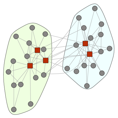
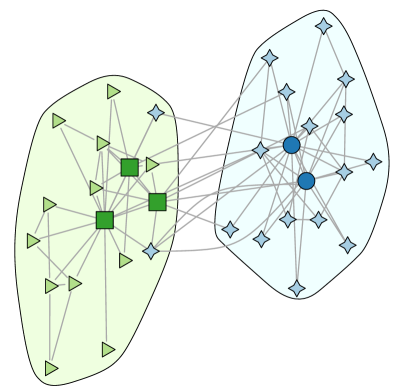
Figure 1: Communities detected by the Bayesian modularity when $K=2$ (left) and $K=4$ (right), with $\alpha=\beta_{1}=\beta_{2}=1/2$. The polygons contain the two groups the karate club was split into; the left one is Mr. Hi’s club, the right one is the Officers’ club. The shapes of the nodes represent the communities selected by the modularities. Figure made using the igraph package (Csardi and Nepusz, 2006).

Zachary (1977) described a karate club which split into two clubs after a conflict over the price of the karate lessons. The new club was led by Mr. Hi, the karate teacher of the original club, while the remainder of the old club stayed under the former Officers’ rule. The data consists of an adjacency matrix for those 34 individuals who interacted with other club members outside club meetings and classes. Each of these individuals’ affiliations after the conflict is known.

The communities selected by the Bayesian modularity for $K=2$ and $K=4$ are given in Figure 1. In both instances, the tabu search led to nearly the same solution for both the Bayesian and likelihood modularities, only differing at one node for $K=4$, which is not surprising in light of Lemma 3.1. For $K=2$, the results of Bickel and Chen (2009) for this data set are recovered. For $K=4$, the partition in Figure 1 yields a higher value of the likelihood modularity than the partition into four classes found by Bickel and Chen (2009), and an even higher value is obtained by switching club member 20 to the second-largest class. This discrepancy is likely due to the heuristic nature of the tabu search algorithm, and for the same reason, it may be the case that improvement over the partitions found by the Bayesian modularity in Figure 1 are possible.

For $K=2$, the communities found by the algorithms do not correspond in the slightest to the two karate clubs, instead grouping the nodes with the highest degrees, corresponding to Mr. Hi, the president of the original club, and their closest supporters, together. Incidentally, this partition is the same as the one returned by the Largest Gaps algorithm of Channarond, Daudin and Robin (2012), which solely uses the degrees of the nodes and discards all other information.

These bad results are no reason to shelve the Bayesian and likelihood modularities, as there is no reason to believe that the two karate clubs form communities in the sense of the stochastic block model. Mr. Hi and the club’s president are clear outliers within their groups, and neither of the algorithms were designed to be robust to such a phenomenon. The communities selected by the modularities are communities in the sense that they form connections within and between the groups in a similar fashion. This sense does not correspond to the social notion of a community in this setting.

The results for four classes unify the social and stochastic senses of community. The prominent members of each of the new clubs are placed into two separate, small, communities. The other members are classified nearly perfectly, with two exceptions. However, one of those exceptional individuals is the only person described by Zachary (1977) as being a supporter of the club’s president before the split, who joined Mr. Hi’s club, making this person’s affiliation up for debate. The second is described as only a weak supporter of Mr. Hi. The increased number of communities allows for some outliers within the social communities, and leads to a more detailed understanding of the dynamics within both of the groups. We essentially recover the two communities, each with a core that is more connective than the remainder of te nodes.

5 Discussion

An advantage of Bayesian modelling is that it does not solely result in an estimator, but in a full posterior distribution. The posterior mode studied in this paper is but one aspect of the posterior, and its good behaviour in terms of consistency is encouraging. Further study into other aspects in the posterior may prove to be fruitful. One possible research direction would be to use the posterior to quantify uncertainty in the estimate of the class labels. A second issue that may be resolved by the Bayesian approach is the question of estimating the number of classes, $K$. This remains an important open question, as noted by Bickel and Chen (2009), despite recent attempts (e.g. Saldana, Yu and Feng (2014), Chen and Lei (2014) and Wang and Bickel (2015)). By introducing a prior on $K$, such as the Poisson-prior suggested by McDaid et al. (2013), the number of communities $K$ can be detected by the posterior.

Appendix A Proofs

After stating some repeatedly used notation, this appendix starts with the proof of Theorem A.1, which is a theorem on weak consistency of the Bayesian modularity. It is followed by a number of supporting Lemmas, after which we proceed to the proof of Theorem 3.2, and some additional supporting Lemmas.

We write $\mathop{\rm diag\,}\nolimits(P)$ for the diagonal of $P$ if $P$ is a matrix, and ${\rm Diag}(f)$ for the diagonal matrix with diagonal $f$ if $f$ is a vector.

A.1 Weak consistency

The following quantities will be used in the course of multiple proofs. The function $H_{P}$, with domain $K\times K$ probability matrices, is given by, for $\tau(u)=u\log u+(1-u)\log(1-u)$,

$$H_{P}(R)=\frac{1}{2}\sum_{a,b}(R\textbf{1})_{a}(R\textbf{1})_{b}\,\tau\left(\frac{(RPR^{T})_{ab}}{(R\textbf{1})_{a}(R\textbf{1})_{b}}\right).$$ (6)

For $\tau_{0}(u)=u\log(u)-u$, define

$$G_{P}(R)=\frac{1}{2}\sum_{a,b}(R\textbf{1})_{a}(R\textbf{1})_{b}\,\tau_{0}\Bigl{(}\frac{(RPR^{T})_{ab}}{(R\textbf{1})_{a}(R\textbf{1})_{b}}\Bigr{)}.$$

The sums defining these functions are over all pairs $(a,b)$ with $1\leq a,b\leq K$, unlike the sums defining the modularities $Q_{B}$ and $Q_{ML}$, which are restricted to $a\leq b$.

Theorem A.1 (weak consistency).

1. If $(P,\pi)$ is fixed and identifiable, then the MAP classifier $\widehat{e}=\arg\max_{z}Q_{B}(e)$ is weakly consistent.

2. If $P=\rho_{n}S$ for $\rho_{n}\to 0$, and $(S,\pi)$ is fixed and identifiable, then the MAP classifier $\widehat{e}=\arg\max_{z}Q_{B}(e)$ is weakly consistent provided $n\rho_{n}\gg(\log n)^{2}$.

Proof.

By Lemma 3.1 the Bayesian modularity $Q_{B}$ is equivalent to the likelihood modularity $Q_{ML}$ up to order $(\log n)/n$. With the notation $\widetilde{O}_{ab}(e)=O_{ab}(e)$ if $a\neq b$, and $\widetilde{O}_{ab}(e)=2O_{ab}(e)$ if $a=b$, the likelihood modularity is in turn equivalent up to the same order to

$$\mathbb{L}(e)=\frac{1}{2n^{2}}\sum_{a,b}n_{a}(e)n_{b}(e)\,\tau\Bigl{(}\frac{\widetilde{O}_{ab}(e)}{n_{a}(e)n_{b}(e)}\Bigr{)}.$$ (7)

Indeed the terms of $Q_{ML}(e)$ for $a<b$ are identical to the sums of the terms of $\mathbb{L}(e)$ for $a<b$ and $a>b$, while for $a=b$ the terms of $Q_{ML}(e)$ and $\mathbb{L}(e)$ differ only subtly: the first uses $n_{aa}(e)=\tfrac{1}{2}n_{a}(e)(n_{a}(e)-1)$, where the second uses $\tfrac{1}{2}n_{a}(e)^{2}$. Thus the difference is bounded in absolute value by the sum over $a$ of (where $e$ is suppressed from the notation)

$$\Bigl{|}\frac{n_{a}^{2}}{2n^{2}}\tau\Bigl{(}\frac{\widetilde{O}_{aa}}{n_{a}^{2}}\Bigr{)}-\frac{n_{a}\bigl{(}n_{a}-1)}{2n^{2}}\tau\Bigl{(}\frac{\widetilde{O}_{aa}}{n_{a}(n_{a}-1)}\Bigr{)}\Bigr{|}\leq\frac{1}{2n}\|\tau\|_{\infty}+\frac{n_{a}^{2}}{2n^{2}}l\Bigl{(}\frac{\widetilde{O}_{aa}}{n_{a}^{2}(n_{a}-1)}\Bigr{)}.$$

where $l(x)=x(1\vee\log(1/x))$, in view of Lemma A.4. We now use that $n_{a}l(u/n_{a})\lesssim\log n_{a}\leq\log n$, for $0\leq u\leq 1$.

Combining the preceding, we conclude that

$$\eta_{n,1}:=\max_{e}|\mathbb{L}(e)-Q_{B}(e)|=\mathcal{O}\left(\frac{\log{n}}{n}\right).$$

Since $Q_{B}(\widehat{e})\geq Q_{B}(Z)$, by the definition of $\widehat{e}$, it follows that $\mathbb{L}(\widehat{e})-\mathbb{L}(Z)\geq-2\eta_{n,1}$. The next step is to replace $\mathbb{L}$ in this equality by an asymptotic value.

For $x$ equal to a big multiple of $(\|P\|_{\infty}^{1/2}\vee n^{-1/2})/n^{1/2}$, the right side of Lemma A.2 tends to zero and hence $\max_{e}\bigl{\|}\widetilde{O}(e)-\mathbb{E}\bigl{(}\widetilde{O}(e)\mid Z\bigr{)}\bigr{\|}_{\infty}/n^{2}$ is of this order in probability. We also have, by Lemma A.3:

$$\max_{e}\Bigl{\|}\frac{1}{n^{2}}\mathbb{E}\bigl{(}\widetilde{O}(e)\mid Z\bigr{)}-R(e,Z)PR(e,Z)^{T}\Bigr{\|}_{\infty}=\max_{e}\frac{1}{n}\bigl{\|}{\rm Diag}(R(e,Z))\mathop{\rm diag\,}\nolimits(P)\bigr{\|}_{\infty}\to 0,$$

as each entry of ${\rm Diag}(R(e,Z))\mathop{\rm diag\,}\nolimits(P)$ is bounded above by one. By Lemma A.4, $\bigl{|}v\tau(x/v)-v\tau(y/v)\bigr{|}\leq l(|x-y|)$, uniformly in $v\in[0,1]$, where $l(x)=x(1\vee\log(1/x))$. It follows that

$$\eta_{n,2}:=\max_{e}\bigl{|}\mathbb{L}(e)-L(e)\bigr{|}=o_{P}\Bigl{(}l\Bigl{(}\frac{\|P\|_{\infty}^{1/2}\vee n^{-1/2}}{n^{1/2}}\Bigr{)}\Bigr{)},$$

for

$$L(e)=\frac{1}{2}\sum_{a,b}f_{a}(e)f_{b}(e)\,\tau\Bigl{(}\frac{(R(e,Z)PR(e,Z)^{T})_{ab}}{f_{a}(e)f_{b}(e)}\Bigr{)}.$$

Combining this with the preceding paragraph, we conclude that $L(\widehat{e})\geq L(Z)-2(\eta_{n,1}+\eta_{n,2})$.

Proof of (i). For given $\delta>0$, let $\mathcal{R}_{\delta}$ be the set of all probability matrices $R$ with

$$\min_{P_{\sigma}}\bigl{\|}P_{\sigma}R-{\rm Diag}(R^{T}\textbf{1})\bigr{\|}_{1}\geq\delta,\qquad\text{ and }\qquad\min_{a:\pi_{a}>0}(R^{T}\textbf{1})_{a}\geq\delta.$$

Here the minimum is taken over the (finite) set of all permutation matrices $P_{\sigma}$ on $K$ labels. Furthermore, set

$$\eta:=\inf_{R\in\mathcal{R}_{\delta}}\bigr{[}H_{P}\bigl{(}{\rm Diag}(R^{T}\textbf{1})\bigr{)}-H_{P}(R)\bigl{]},$$

where $H_{P}$ is as defined in $\eqref{eq:HP}$. Because $\mathcal{R}_{\delta}$ is compact and the maps $R\mapsto H_{P}(R)$ and $R\mapsto{\rm Diag}(R^{T}\textbf{1})$ are continuous, the infimum in the display is assumed for some $R\in\mathcal{R}_{\delta}$. Because no $R\in\mathcal{R}_{\delta}$ can be transformed into a diagonal element by permuting rows and every $R\in\mathcal{R}_{\delta}$ has a nonzero element in every column $a$ with $\pi_{a}>0$, Lemma A.5 shows that $\eta_{n}>0$.

Because $L(e)=H_{P}(R(e,Z))$ for every $e$, and $R(Z,Z)={\rm Diag}(f(Z))={\rm Diag}(R(\widehat{e},Z)^{T}\textbf{1})$, we conclude that

$$H_{P}({\rm Diag}(R(\widehat{e},Z)^{T}\textbf{1}))-H_{P}(R(\widehat{e},Z))\leq 2(\eta_{n,1}+\eta_{n,2}).$$

If $2(\eta_{n,1}+\eta_{n,2})$ is smaller than $\eta_{n}$, then it follows that $R(\widehat{e},Z)$ cannot be contained in $\mathcal{R}_{\delta}$. Since $R(\widehat{e},Z)^{T}\textbf{1}=f(Z)\stackrel{{\scriptstyle P}}{{\to}}\pi$, by the law of large numbers, for sufficiently small $\delta>0$ this must be because $R(\widehat{e},Z)$ fails the first requirement defining $\mathcal{R}_{\delta}$. That is, $\|P_{\sigma}R(\widehat{e},Z)-{\rm Diag}(f(Z))\|_{1}\leq\delta$ for some permutation matrix $P_{\sigma}$. As this is true eventually for any $\delta>0$, it follows that $\min_{P_{\sigma}}\|P_{\sigma}R(\widehat{e},Z)-{\rm Diag}(\pi)\|_{1}\stackrel{{\scriptstyle P}}{{\to}}0$.

Proof of (ii). In view of Lemma A.6, the number $\eta=\eta_{n}$, which now depends on $n$, is now bounded below by $\rho_{n}$ times a positive number that depends on $(S,\pi)$. The preceding argument goes through provided $\eta_{n,1}+\eta_{n,2}$ is of smaller order than $\eta_{n}$. This leads to $l\bigl{(}\sqrt{\rho_{n}/n}\bigr{)}+\log(n)/n\ll\rho_{n}$, or $(\rho_{n}/n)\log^{2}\bigl{(}n/(\rho_{n}\|S\|_{\infty})\bigr{)}\ll\rho_{n}^{2}$. ∎

Lemma A.2.

Let $\widetilde{O}_{ab}(e)=O_{ab}(e)$ if $a\neq b$, and $\widetilde{O}_{ab}(e)=2O_{ab}(e)$ if $a=b$. For any $x>0$,

$$\mathbb{P}\Bigl{(}\max_{e}\bigl{\|}\widetilde{O}(e)-\mathbb{E}\bigl{(}\widetilde{O}(e)\mid Z\bigr{)}\bigr{\|}_{\infty}>xn^{2}\Bigr{)}\leq 2K^{n+2}e^{-x^{2}n^{2}/(8\|P\|_{\infty}+4x/3)}.$$

Proof.

This Lemma is adapted from Lemma 1.1 in Bickel and Chen (2009). There are $K^{n}$ possible values of $e$ and $\|\cdot\|_{\infty}$ is the maximum of the $K^{2}$ entries in the matrix. We use the union bound to pull these maxima out of the probability, giving the factor $K^{n+2}$ on the right. Next it suffices to bound the tail probability of each variable

$$\widetilde{O}_{ab}(e)-\mathbb{E}\bigl{(}\widetilde{O}_{ab}(e)\mid Z\bigr{)}=\sum_{i,j}\bigl{(}A_{ij}-\mathbb{E}(A_{ij}\mid Z)\bigr{)}(\textbf{1}\{e_{i}=a,e_{j}=b\}+\textbf{1}\{e_{i}=b,e_{j}=a\}).$$

The $n_{ab}(e)$ variables in this sum are conditionally independent given $Z$, take values in $[-2,2]$, and have conditional mean zero given $Z$ and conditional variance bounded by $4\mathop{\rm var}\nolimits(A_{ij}\mid Z)\leq 4P_{Z_{i}Z_{j}}(1-P_{Z_{i}Z_{j}})\leq 4\|P\|_{\infty}$. Thus we can apply Bernstein’s inequality to find that

$$\mathbb{P}\Bigl{(}\bigl{|}\widetilde{O}_{ab}(e)-\mathbb{E}\bigl{(}\widetilde{O}_{ab}(e)\mid Z\bigr{)}\bigr{|}>xn^{2}\Bigr{)}\leq 2e^{-x^{2}n^{4}/(8n_{ab}(e)\|P\|_{\infty}+4xn^{2}/3)}.$$

Finally we use the crude bound $n_{ab}(e)\leq n^{2}$ and cancel one factor $n^{2}$. ∎

Lemma A.3.

Define $\widetilde{O}_{ab}(e)=O_{ab}(e)$ if $a\neq b$, and $\widetilde{O}_{ab}(e)=2O_{ab}(e)$ if $a=b$. Then, for $R(e,Z)$ as defined in (2),

$$\mathbb{E}(\widetilde{O}_{ab}\mid Z)=n^{2}R(e,Z)PR(e,Z)^{T}-n{\rm Diag}(R(e,Z)\mathop{\rm diag\,}\nolimits(P)).$$

Proof.

A similar expression, not taking into account the absence of self-loops, appears in Bickel and Chen (2009).

$$\mathbb{E}(\widetilde{O}_{ab}(e)\mid Z=c)=\sum_{i\neq j}P_{c_{i}c_{j}}\textbf{1}\{e_{i}=a,e_{j}=b\}$$

$$\quad=\sum_{a^{\prime},b^{\prime}}P_{a^{\prime}b^{\prime}}\sum_{i\neq j}\textbf{1}\{c_{i}=a^{\prime},c_{j}=b^{\prime}\}\textbf{1}\{e_{i}=a,e_{j}=b\}$$

$$\quad=\sum_{a^{\prime},b^{\prime}}P_{a^{\prime}b^{\prime}}\sum_{i,j}\textbf{1}\{c_{i}=a^{\prime},c_{j}=b^{\prime}\}\textbf{1}\{e_{i}=a,e_{j}=b\}-\delta_{ab}\sum_{a^{\prime}}P_{a^{\prime}a^{\prime}}\textbf{1}\{c_{i}=a^{\prime}\}\textbf{1}\{e_{i}=a\}$$

$$\quad=n^{2}\sum_{a^{\prime},b^{\prime}}P_{a^{\prime}b^{\prime}}R_{aa^{\prime}}(e,c)R_{bb^{\prime}}(e,c)-\delta_{ab}n\sum_{a^{\prime}}P_{a^{\prime}a^{\prime}}R_{aa^{\prime}}(e,c).$$

∎

Lemma A.4.

The function $\tau:[0,1]\to\mathbb{R}$ satisfies $|\tau(x)-\tau(y)|\leq l(|x-y|)$, for $l(x)=2x(1\vee\log(1/x))$.

Proof.

Write the difference between $x\log{x}$ and $y\log{y}$ as $|\int_{x}^{y}(1+\log s)\,ds|$. The function $s\mapsto 1+\log s$ is strictly increasing on $[0,1]$ from $-\infty$ to 1 and changes sign at $s=e^{-1}$. Therefore the absolute integral is bounded above by the maximum of

$$-\int_{0}^{|x-y|\wedge e^{-1}}(1+\log s)\,ds =-(|x-y|\wedge e^{-1})\log{|x-y|\wedge e^{-1}}$$

$$\int_{1-|x-y|\vee e^{-1}}^{1}(1+\log s)\,ds \leq|x-y|.$$

∎

Proof of Lemma 3.1

Proof.

The second assertion of the lemma follows from the first and the fact that $\max_{e}Q_{P}(e)\lesssim(\log n)/n$. It suffices to prove the first assertion.

Recall that the Bayesian modularity is given by

$$n^{2}Q_{B}(e)=\sum_{a\leq b}\log B\left(O_{ab}(e)+\tfrac{1}{2},n_{ab}(e)-O_{ab}(e)+\tfrac{1}{2}\right)+\sum_{a}\log\Gamma(n_{a}(e)+\alpha).$$ (8)

We shall show that the first sum on the right is equivalent to $Q_{ML}(e)$, and the second sum is equivalent to $Q_{P}(e)$. We show this by comparing the sums defining the various modularities term by term. For clarity we shall suppress the argument $e$. We will repeatedly use the following bound from (Robbins, 1955): for $n\in\mathbb{N}_{\geq 1}$,

$$\Gamma(n+1)=\sqrt{2\pi}n^{n+1/2}e^{-n}e^{a_{n}},$$ (9)

with $(12n+1)^{-1}\leq a_{n}\leq(12n)^{-1}$, as well as the fact that $\Gamma(s)$ is monotone increasing for $s\geq 3/2$. In addition, we will bound remainder terms by using the inequality $x\log((x+c)/x)\leq c$ for $c\geq 0$ and the fact that $x\log((x-1)/x)$ is bounded for $x>1$.

First sum of (8).
Upper bound, case 1: $O_{ab}\neq 0$ and $n_{ab}\neq O_{ab}$
We apply (9):

$$\log B(O_{ab}+\beta_{1},n_{ab}-O_{ab}+\beta_{2})\leq\log\frac{\Gamma(O_{ab}+\lfloor{\beta_{1}}\rfloor+1)\Gamma(n_{ab}-O_{ab}+\lfloor{\beta_{2}}\rfloor+1)}{\Gamma(n_{ab}+\lfloor{\beta_{1}+\beta_{2}}\rfloor)}$$

$$=O_{ab}\log\left(\frac{O_{ab}+\lfloor{\beta_{1}}\rfloor}{n_{ab}+\lfloor{\beta_{1}+\beta_{2}}\rfloor-1}\right)+(n_{ab}-O_{ab})\log\left(\frac{n_{ab}-O_{ab}+\lfloor{\beta_{2}}\rfloor}{n_{ab}+\lfloor{\beta_{1}+\beta_{2}}\rfloor-1}\right)$$

$$\quad+(\lfloor{\beta_{1}}\rfloor+1/2)\log(O_{ab}+\lfloor{\beta_{1}}\rfloor)+(\lfloor{\beta_{2}}\rfloor+1/2)\log(n_{ab}-O_{ab}+\lfloor{\beta_{2}}\rfloor)$$

$$\quad-(\lfloor{\beta_{1}+\beta_{2}}\rfloor-1/2)\log(n_{ab}+\lfloor{\beta_{1}+\beta_{2}}\rfloor-1)+\log\sqrt{2\pi}-\lfloor{\beta_{1}}\rfloor-\lfloor{\beta_{2}}\rfloor+\lfloor{\beta_{1}+\beta_{2}}\rfloor-1$$

$$\quad+\alpha_{ab}+\beta_{ab}-\gamma_{ab},$$

where $\alpha_{ab},\beta_{ab}$ and $\gamma_{ab}$ are bounded by constants. By the inequality $x\log((x+c)/x)\leq c$ for $c\geq 0$, and the fact that $x\log((x-1)/x)$ is bounded for $x>1$, we find the upper bound:

$$\log B(O_{ab}+\beta_{1},n_{ab}-O_{ab}+\beta_{2})\leq n_{ab}\tau\left(\frac{O_{ab}}{n_{ab}}\right)+O(\log{n_{ab}}).$$

Upper bound, case 2: $n_{ab}=1$ and $O_{ab}=0$ or $n_{ab}=O_{ab}$, or $n_{ab}=0$
In both cases, the corresponding term of the likelihood modularity vanishes, whereas the contribution of the Bayesian modularity is either $\log B(1+\beta_{1},\beta_{2})$, $\log(\beta_{1},1+\beta_{2})$, or $\log B(\beta_{1},\beta_{2})$.

Upper bound, case 3: $n_{ab}\geq 2$ and $O_{ab}=0$ or $n_{ab}=O_{ab}$
Again, the corresponding term of the likelihood modularity vanishes. We show the computations for the case $n_{ab}=O_{ab}$; for the case $O_{ab}=0$, switch $\beta_{1}$ and $\beta_{2}$. By (9):

$$\log B(O_{ab}+\beta_{1},n_{ab}-O_{ab}+\beta_{2})=\log B(n_{ab}+\beta_{1},\beta_{2})\leq\log\frac{\Gamma(n_{ab}+\lfloor{\beta_{1}}\rfloor+1)\Gamma(\beta_{2})}{\Gamma(n_{ab}+\lfloor{\beta_{1}+\beta_{2}}\rfloor)}$$

$$=(n_{ab}+\lfloor{\beta_{1}}\rfloor)\log\left(\frac{n_{ab}+\lfloor{\beta_{1}}\rfloor}{n_{ab}+\lfloor{\beta_{1}+\beta_{2}}\rfloor}\right)+(1/2)\log(n_{ab}+\lfloor{\beta_{1}}\rfloor)$$

$$\quad-(\lfloor{\beta_{1}+\beta_{2}}\rfloor+1/2)\log(n_{ab}+\lfloor{\beta_{1}+\beta_{2}}\rfloor)+\log\Gamma(\beta_{2})+\lfloor{\beta_{1}+\beta_{2}}\rfloor-1+\delta_{ab}-\epsilon_{ab},$$

where $\delta_{ab}$ and $\epsilon_{ab}$ are bounded by constants. Arguing as before, the first term is bounded, while the remainder is of order $\log(n_{ab})$. A lower bound is found analogously.

Lower bound The computations for the lower bound are completely analogous, except that we require $O_{ab}+\beta_{1}\geq 2$ and $n_{ab}-O_{ab}+\beta_{2}\geq 2$. We study four cases. The cases (1) $O_{ab}\geq 2$ and $n_{ab}-O_{ab}\geq 2$, (2) $n_{ab}=0$ and (3) $n_{ab}>0$ and $n_{ab}=O_{ab}$ or $O_{ab}=0$ are similar to cases 1, 2 and 3 respectively of the upper bound. The fourth case is $n_{ab}-O_{ab}=1$ and $O_{ab}\geq 2$, or $O_{ab}=1$ and $n_{ab}-O_{ab}\geq 1$. In both instances, the likelihood modularity is equality to a bounded term minus $\log{n_{ab}}$. By similar calculations as before, the Bayesian modularity is of the order $\log{n_{ab}}$ as well.

Conclusion We find:

$$\sum_{a\leq b}\log B(O_{ab}+\beta_{1},n_{ab}-O_{ab}+\beta_{2})=\sum_{a\leq b}n_{ab}\tau\left(\frac{O_{ab}}{n_{ab}}\right)+O(\log{n}).$$

Second sum of (8).
We consider three cases. If $n_{a}+\lfloor{\alpha}\rfloor=0$, then $\alpha>0$, implies $n_{a}=0$, in which case $\log\Gamma(n_{a}+\alpha)=\log\Gamma(\alpha)$, which is bounded. In case $n_{a}+\lfloor{\alpha}\rfloor=1$, the term $\log\Gamma(n_{a}+\alpha)$ is equal to either $\log\Gamma(1+\alpha)$ or $\log\Gamma(\alpha)$ and thus bounded as well. For the case $n_{a}+\lfloor{\alpha}\rfloor\geq 2$, we study the upper bound $\Gamma(n_{a}+\alpha)\leq\Gamma(n_{a}+\lfloor{\alpha}\rfloor+1)$ and the lower bound $\Gamma(n_{a}+\alpha)\geq\Gamma(n_{a}+\lfloor{\alpha}\rfloor)$. By applying (9) in both cases, we conclude:

$$\sum_{a}\log\Gamma(n_{a}+\alpha)=\sum_{a:n_{a}+\lfloor{\alpha}\rfloor\geq 2}n_{a}\log n_{a}-n+O(\log n).$$

∎

Lemma A.5.

For any probability matrix $R$,

$$H_{P}(R)\leq H_{P}({\rm Diag}(R^{T}\textbf{1})\bigr{)}.$$ (10)

Furthermore, if $(P,\pi)$ is identifiable and the columns of $R$ corresponding to positive coordinates of $\pi$ are not identically zero, then the inequality is strict unless $P_{\sigma}R$ is a diagonal matrix for some permutation matrix $P_{\sigma}$.

Proof.

This Lemma is related to the proof that the likelihood modularity is consistent given in Bickel and Chen (2009). This proof however rests on their incorrect Lemma 3.1, and thus we provide full details on how the argument can be adapted to avoid the use of their Lemma 3.1 altogether.

For $R$ a diagonal matrix the numbers $(RPR^{T})_{ab}/(R\textbf{1})_{a}(R\textbf{1})_{b}$ reduce to $P_{ab}$. Consequently, by the definition of $H_{P}$,

$$H_{P}\bigl{(}{\rm Diag}(f)\bigr{)}=\sum_{a,b}f_{a}f_{b}\,\tau(P_{ab}).$$ (11)

For a general matrix $R$, by inserting the definition of $\tau$,

$$H_{P}(R) =\sum_{a,b}(RPR^{T})_{ab}\log\frac{(RPR^{T})_{ab}}{(R\textbf{1})_{a}(R\textbf{1})_{b}}$$

$$\qquad\qquad+\sum_{a,b}\bigl{(}(R\textbf{1})_{a}(R\textbf{1})_{b}-(RPR^{T})_{ab}\bigr{)}\log\Bigl{(}1-\frac{(RPR^{T})_{ab}}{(R\textbf{1})_{a}(R\textbf{1})_{b}}\Bigr{)}.$$

Because $(R\textbf{1})_{a}(R\textbf{1})_{b}-(RPR^{T})_{ab}=(R(1-P)R^{T})_{ab}$, with $1$ the $(K\times K)$-matrix with all coordinates equal to 1, we can rewrite this as

$$\sum_{a,b}\sum_{a^{\prime},b^{\prime}}R_{aa^{\prime}}R_{bb^{\prime}}\biggl{[}P_{a^{\prime}b^{\prime}}\log\frac{(RPR^{T})_{ab}}{(R\textbf{1})_{a}(R\textbf{1})_{b}}+(1-P_{a^{\prime}b^{\prime}})\log\Bigl{(}1-\frac{(RPR^{T})_{ab}}{(R\textbf{1})_{a}(R\textbf{1})_{b}}\Bigr{)}\biggr{]}.$$

By the information inequality for two-point measures, the expressions in square brackets becomes bigger when $(RPR^{T})_{ab}/(R\textbf{1})_{a}(R\textbf{1})_{b}$ is replaced by $P_{a^{\prime}b^{\prime}}$, with a strict increase unless these two numbers are equal. After making this substitution the terms in square brackets becomes $\tau(P_{a^{\prime}b^{\prime}})$, and we can exchange the order of the two (double) sums and perform the sum on $(a,b)$ to write the resulting expression as

$$\sum_{a^{\prime},b^{\prime}}(R^{T}\textbf{1})_{a^{\prime}}(R^{T}\textbf{1})_{b^{\prime}}\tau(P_{a^{\prime}b^{\prime}})=H_{P}\bigl{(}{\rm Diag}(R^{T}\textbf{1})\bigr{)}.$$

This proves the first assertion (10) of the lemma.

If $R$ attains equality, then also for every permutation matrix $P_{\sigma}$, by the equality $H_{P}(P_{\sigma}R)=H_{P}(R)$ and the fact that $(P_{\sigma}R)^{T}\textbf{1}=R^{T}\textbf{1}$, we have

$$H_{P}(P_{\sigma}R)=H_{P}\bigl{(}{\rm Diag}((P_{\sigma}R)^{T}\textbf{1})\bigr{)}.$$ (12)

We shall show that if $R$ satisfies this equality and $P_{\sigma}R$ has a positive diagonal, then $P_{\sigma}R$ is in fact diagonal. Furthermore, we shall show that there exists $P_{\sigma}$ such that $P_{\sigma}R$ has a positive diagonal.

Fix some $(P_{\sigma})_{m}$ that maximizes the number of positive diagonal elements of $P_{\sigma}R$ over all permutation matrices $P_{\sigma}$, and denote $\bar{R}=(P_{\sigma})_{m}R$. Because the information inequality is strict, the preceding argument shows that (12) can be true for $P_{\sigma}=(P_{\sigma})_{m}$ (giving $P_{\sigma}R=\bar{R}$) only if

$$P_{a^{\prime}b^{\prime}}=\frac{(\bar{R}P\bar{R}^{T})_{ab}}{(\bar{R}\textbf{1})_{a}(\bar{R}\textbf{1})_{b}},\qquad\text{whenever }\bar{R}_{aa^{\prime}}\bar{R}_{bb^{\prime}}>0.$$ (13)

Denote the matrix on the right of the equality by $Q$.

If $\bar{R}$ has a completely positive diagonal, then we can choose $a=a^{\prime}$ and $b=b^{\prime}$ and find from equation (13), that $P_{ab}=Q_{ab}$, for every $a,b$. If also $\bar{R}_{aa^{\prime}}>0$, then we can also choose $b=b^{\prime}$ and find that $P_{a^{\prime}b}=Q_{ab}$, for every $b$. Thus the $a$th and $a^{\prime}$th rows of $P$ are identical. Since all rows of $P$ are different by assumption, it follows that no $a\not=a^{\prime}$ with $\bar{R}_{aa^{\prime}}>0$ exists.

If $\bar{R}$ does not have a fully positive diagonal, then the submatrix of $\bar{R}$ obtained by deleting the rows and columns corresponding to positive diagonal elements must be the zero matrix, since otherwise we might permute the remaining rows and create an additional nonzero diagonal element, contradicting that $(P_{\sigma})_{m}$ already maximized this number. If $I$ and $I^{c}$ are the sets of indices of zero and nonzero diagonal elements, then the preceding observation is that $\bar{R}_{ij}$ is zero for every $i,j\in I$. If $\pi>0$, then we need to consider only $R$ with nonzero columns. For $i\in I$ a nonzero element in the $i$th column of $\bar{R}$ must be located in the rows with label in $I^{c}$: for every $i\in I$ there exists $k_{i}\in I^{c}$ with $\bar{R}_{k_{i}i}>0$. Then, for $i,j\in I$,

• for $a=k_{i}$, $b=k_{j}$, $a^{\prime}=i$, $b^{\prime}=j$, equation (13) implies $Q_{k_{i}k_{j}}=P_{ij}$.

• for $a=k_{i}$, $b\in I^{c}$, $a^{\prime}=i$, $b^{\prime}=b$, equation (13) implies $Q_{k_{i}b}=P_{ib}$.

• for $a=k_{i}$, $b\in I^{c}$, $a^{\prime}=k_{i}$, $b^{\prime}=b$, equation (13) implies $Q_{k_{i}b}=P_{k_{i}b}$.

We combine these three assertions to conclude that, for $a,i\in I$ and $b\in I^{c}$,

$$P_{ai} =P_{ia}\stackrel{{\scriptstyle(1)}}{{=}}Q_{k_{i}k_{a}}\stackrel{{\scriptstyle(2)}}{{=}}P_{ik_{a}}=P_{k_{a}i},$$

$$P_{ab} \stackrel{{\scriptstyle(2)}}{{=}}Q_{k_{a}b}\stackrel{{\scriptstyle(3)}}{{=}}P_{k_{a}b}.$$

Together these imply that the $a$th and the $k_{a}$th row of $P$ are equal. Since by assumption they are not (if $\pi>0$), this case can actually not exist (i.e. $k=0$).

Finally if $\pi_{a}=0$ for some $a$, then we follow the same argument, but we match only every column $i\in I$ with $\pi_{i}>0$ to a row $k_{i}\in I^{c}$. By the assumption on $R$ such $k_{i}$ exist, and the construction results in two rows of $P$ that are identical in the coordinates with $\pi_{a}>0$.∎

Lemma A.6.

For any fixed $(K\times K)$-matrix $P$ with elements in $[0,1]$, uniformly in probability matrices $R$, as $\rho_{n}\rightarrow 0$,

$$\frac{1}{\rho_{n}}\Bigl{(}H_{\rho_{n}P}({\rm Diag}(R^{T}\textbf{1})\bigr{)}-H_{\rho_{n}P}(R)\Bigr{)}\rightarrow G_{P}({\rm Diag}(R^{T}\textbf{1})\bigr{)}-G_{P}(R).$$ (14)

Furthermore, if $(P,\pi)$ is identifiable and the columns of $R$ corresponding to positive coordinates of $\pi$ are not identically zero, then the right side is strictly positive unless $SR$ is a diagonal matrix for some permutation matrix $S$.

Proof.

From the fact that $|(1-u)\log(1-u)+u|\leq u^{2}$, for $0\leq u\leq 1$, it can be verified that, $\bigl{|}\rho_{n}^{-1}\tau(\rho_{n}u)-\bigl{(}u\log\rho_{n}+\tau_{0}(u)\bigr{)}\bigr{|}\leq\rho_{n}\rightarrow 0$, uniformly in $0\leq u\leq 1$. It follows that, uniformly in $R$,

$$\frac{1}{\rho_{n}}H_{\rho_{n}P}(R)=\log\rho_{n}\sum_{a,b}(RPR^{T})_{ab}+\sum_{a,b}(R\textbf{1})_{a}(R\textbf{1})_{b}\tau_{0}\Bigl{(}\frac{(RPR^{T})_{ab}}{(R\textbf{1})_{a}(R\textbf{1})_{b}}\Bigr{)}+O(\rho_{n}).$$

The first term on the right is equal to $\log\rho_{n}(R^{T}\textbf{1})^{T}P(R^{T}\textbf{1})$, and hence is the same for $R$ and ${\rm Diag}(R^{T}\textbf{1})$. Thus this term cancels on taking the difference to form the left side of (14), and hence (14) follows.

The right side of (14) is nonnegative, because the left side is, by Lemma A.5. This fact can also be proved directly along the lines of the proof of Lemma A.5, as follows. Write

$$G_{P}(R)=\sum_{a,b}\sum_{a^{\prime},b^{\prime}}R_{aa^{\prime}}R_{bb^{\prime}}\Bigl{[}P_{a^{\prime}b^{\prime}}\log\frac{(RPR^{T})_{ab}}{(R\textbf{1})_{a}(R\textbf{1})_{b}}-\frac{(RPR^{T})_{ab}}{(R\textbf{1})_{a}(R\textbf{1})_{b}}\Bigr{]}.$$

By the information inequality for two Poisson distributions the term in square brackets becomes bigger if $(RPR^{T})_{ab}/(R\textbf{1})_{a}(R\textbf{1})_{b}$ is replaced by $P_{a^{\prime}b^{\prime}}$. It then becomes $\tau_{0}(P_{a^{\prime}b^{\prime}})$ and the double sum on $(a,b)$ can be executed to see that the resulting bound is $G_{P}\bigl{(}{\rm Diag}(R^{T}\textbf{1})\bigr{)}$. Furthermore, the inequality is strictly unless (13) holds, with $\bar{R}=R$. Since also $G_{P}(P_{\sigma}R)=G_{P}(R)$, for every permutation matrix $P_{\sigma}$, the final assertion of the lemma is proved by copying the proof of Lemma A.5. ∎

A.2 Strong consistency

We need slightly adapted versions of the function $H_{P}$, given by, with $\delta_{ab}$ equal to 1 or 0 if $a=b$ or not,

$$H_{P,n}(R) =\frac{1}{2}\sum_{a,b}(R\textbf{1})_{a}\bigl{(}(R\textbf{1})_{b}-\delta_{ab}/n\bigr{)}\,\tau\Bigl{(}\frac{(RPR^{T})_{ab}-\delta_{ab}\sum_{k}P_{kk}R_{ka}/n}{(R\textbf{1})_{a}\bigl{(}(R\textbf{1})_{b}-\delta_{ab}/n\bigr{)}}\Bigr{)}.$$ (15)

For given functions $t_{ab}:[0,1]\to\mathbb{R}$, let $X(e)$ be the $K\times K$ matrix with entries

$$X_{ab}(e)=t_{ab}\Bigl{(}\frac{\widetilde{O}_{ab}(e)}{n^{2}}\Bigr{)}-t_{ab}\Bigl{(}\frac{\mathbb{E}(\widetilde{O}_{ab}(e)\mid Z)}{n^{2}}\Bigr{)}.$$ (16)

Proof of Theorem 3.2 [strong consistency]

Proof.

(i). By Theorem A.1, $\widehat{e}$ is weakly consistent, and hence with probability tending to one it belongs to the set of classifications $e$ such that the fractions $f(e)$ are close to $\pi$, and the matrices $R(e,Z)$ are close to ${\rm Diag}(\pi)$ after the appropriate permutation of the labels (that is, of rows of $R(e,Z)$). Therefore, it is no loss of generality to assume that $\widehat{e}$ is restricted to this set. By Lemmas A.2 and A.3, the matrices $\widetilde{O}(e)/n^{2}$ are then close to $R(e,Z)PR(e,Z)^{T}\rightarrow{\rm Diag}(\pi)P{\rm Diag}(\pi)$, and hence are bounded away from zero and one if $P$ has this property.

If $\widehat{e}$ and $Z$ differ at $m$ nodes, then $\widehat{e}$ belongs to the set of $e$ with $\|R(Z,Z)-R(e,Z)\|_{1}=m(2/n)$, by Lemma 2.1. In that case $Q_{B}(e)\geq Q_{B}(Z)$, for some $e$ in this set, and hence by Lemma 3.1 $Q_{ML}(e)-Q_{ML}(Z)+Q_{P}(e)-Q_{P}(Z)\geq-\eta_{n}$, for some $\eta_{n}$ of order $(\log n)/n^{2}$. It follows that:

$$\bigl{[}Q_{ML}(e)-H_{P,n}\bigl{(}R(e,Z)\bigr{)}\bigr{]}-\bigl{[}Q_{ML}(Z)-H_{P,n}\bigl{(}R(Z,Z)\bigr{)}\bigr{]}$$

$$\qquad\qquad\geq H_{P,n}\bigl{(}R(Z,Z)\bigr{)}-H_{P,n}\bigl{(}R(e,Z)\bigr{)}-|Q_{P}(e)-Q_{P}(Z)|-\eta_{n}.$$ (17)

The first term on the right is bounded below by a multiple of $m/n$, by Lemmas  A.7 and 2.1. Because $(x+\alpha)\log x-(y+\alpha)\log y=\int_{x}^{y}(\log s+(s+\alpha)/s)\,ds$ is bounded in absolute value by a multiple of $|x-y|\log(x\vee y)$, if $\alpha\geq 0$ and $x,y>0$, the second term $-|Q_{P}(e)-Q_{P}(Z)|$ is bounded below by a multiple of $m(\log n)/n^{2}$, for some positive constant $C_{2}$, which is of smaller order than $m/n$. We conclude that the left side of (17) is bounded below by $C_{1}m/n$. The left side is $\sum_{a,b}\bigl{(}X_{ab}(e)-X_{ab}(Z)\bigr{)}$, for $X$ defined in (16) and $t$ the function with coordinates $t_{ab}(o)=f_{a}(e)\bigl{(}f_{b}(e)-\delta_{ab}/n\bigr{)}\tau\bigl{(}o/f_{a}(e)\bigl{(}f_{b}(e)-\delta_{ab}/n\bigr{)}\bigr{)}$. Because we restrict $e$ to classifications such that $O_{ab}(e)/n_{ab}(e)$ and $f_{a}(e)f_{b}(e)$ are bounded away from zero and one, only the values of the function $\tau$ on an open interval strictly within $(0,1)$ matter. On any such interval $\tau$ has uniformly bounded derivatives, and hence the bound of Lemma A.10 is valid. Thus we find that

$$\Pr\bigl{(}\#(i:\widehat{e}_{i}\not=Z_{i})=m\bigr{)} \leq\Pr\Bigl{(}\sup_{e:\#(i:e_{i}\not=Z_{i})\leq m}\bigl{\|}X(e)-X(Z)\bigr{\|}_{\infty}\geq\frac{C_{1}m}{n}\Bigr{)}$$

$$\lesssim K^{m}\binom{n}{m}e^{-cm^{2}/(m\|P\|_{\infty}/n+m/n)}$$

$$\leq e^{m\log(Kne/m)-c_{1}mn}.$$

The sum of the right side over $m=1,\ldots,n$ tends to zero.

(ii). We follow the proof for (i), but in (17) use that $H_{P,n}\bigl{(}R(Z,Z)\bigr{)}-H_{P,n}\bigl{(}R(e,Z)\bigr{)}\geq\rho_{n}C\|R(Z,Z)-R(e,Z)\|_{1}\geq\rho_{n}C2m/n$, by Lemma A.9. Since $\rho_{n}\gg(\log n)/n$ by assumption, we have that the contribution $m(\log n)/n^{2}$ of $Q_{P}(e)-Q_{P}(Z)$ is still negligible and hence $\rho_{n}C2m/n$ is a lower bound for the left side of (17). As a bound on the left side of the preceding display, we then obtain

$$\sum_{m=1}^{n}K^{m}\binom{n}{m}e^{-c_{2}\rho_{n}^{2}m^{2}/(m\rho_{n}/n+\rho_{n}m/n)}\leq\sum_{m=1}^{n}e^{m\log(Kne/m)-c_{3}\rho_{n}mn}.$$

This sum tends to zero provided that $n\rho_{n}\gg\log n$. ∎

Lemma A.7.

If $P$ is fixed and symmetric and every pair of rows of $P$ is different and $0<P<1$ and $\pi>0$, then, for sufficiently small $\delta>0$,

$$\liminf_{n\rightarrow\infty}\inf_{0<\|R-{\rm Diag}(\pi)\|<\delta}\frac{H_{P,n}\bigl{(}{\rm Diag}(R^{T}\textbf{1})\bigr{)}-H_{P,n}(R)}{\|{\rm Diag}(R^{T}\textbf{1})-R\|}>0.$$ (18)

Proof.

We can reparametrize the $K\times K$ matrices $R$ by the pairs $(R^{T}\textbf{1},R-{\rm Diag}(R^{T}\textbf{1}))$, consisting of the $K$ vector $f=R^{T}\textbf{1}$ and the $K\times K$ matrix $R-{\rm Diag}(R^{T}\textbf{1})$. The latter matrix is characterized by having nonnegative off-diagonal elements and zero column sums, and can be represented in the basis consisting of all $K\times K$ matrices $\Delta_{bb^{\prime}}$, for $b\not=b^{\prime}$, defined by: $(\Delta_{bb^{\prime}})_{b^{\prime}b^{\prime}}=-1$, $(\Delta_{bb^{\prime}})_{bb^{\prime}}=1$ and $(\Delta_{bb^{\prime}})_{aa^{\prime}}=0$, for all other entries $(a,a^{\prime})$, i.e. the $b^{\prime}$th column of $\Delta_{bb^{\prime}}$ has a $1$ in the $b$th coordinate and a $-1$ on the $b^{\prime}$th coordinate and all its other columns are zero. Given any matrix $R\geq 0$ the matrix $R-{\rm Diag}(R^{T}\textbf{1})$ can be decomposed as

$$R-{\rm Diag}(R^{T}\textbf{1})=\sum_{b\not=b^{\prime}}{\lambda}_{bb^{\prime}}\Delta_{bb^{\prime}},$$

for ${\lambda}_{bb^{\prime}}=R_{bb^{\prime}}\geq 0$. Since every $\Delta_{bb^{\prime}}$ has exactly one nonzero off-diagonal element, which is equal to 1, and in a different location for each $b\not=b$, the sum of the off-diagonal elements of the matrix on the right side is $\sum_{b,b^{\prime}}{\lambda}_{bb^{\prime}}$. Because the sum of all its elements is zero, it follows that its sum of absolute elements is given by $\|R-{\rm Diag}(R^{T}\textbf{1})\|_{1}=2\sum_{b\not=b^{\prime}}{\lambda}_{bb^{\prime}}$.

Thus we obtain a further reparametrization $R\leftrightarrow(f,{\lambda})$, in which $R={\rm Diag}(f)+\sum_{b\not=b^{\prime}}{\lambda}_{bb^{\prime}}\Delta_{bb^{\prime}}$. For given $P$, $f$ and $n$, define the function

$$G({\lambda})=H_{P,n}\Bigl{(}{\rm Diag}(f)+\sum_{b\not=b^{\prime}}{\lambda}_{bb^{\prime}}\Delta_{bb^{\prime}}\Bigr{)}.$$

Then we would like to show that there exists $C$ such that

$$\frac{H_{P,n}({\rm Diag}(R^{T}\textbf{1}))-H_{P,n}(R)}{\|R-{\rm Diag}(R^{T}\textbf{1})\|_{1}}=\frac{G(0)-G({\lambda})}{2\sum_{b\not=b^{\prime}}{\lambda}_{bb^{\prime}}} \geq C>0,$$

for every $f$ in a neighbourhood of $\pi$, ${\lambda}$ in a neighbourhood of $0$ intersected with $\{{\lambda}:{\lambda}\geq 0\}$, and every sufficiently large $n$. The numerator in the quotient is $f(0)-f(1)$ for the function $f(s)=G(s{\lambda})$. Writing this difference in the form $-f^{\prime}(0)-\int_{0}^{1}\bigl{(}f^{\prime}(s)-f^{\prime}(0)\bigr{)}\,ds$ gives that the numerator is equal to

$$-\nabla G(0)^{T}{\lambda}-\int_{0}^{1}\bigl{(}\nabla G(s{\lambda})-\nabla G(0))\bigr{)}^{T}\,ds\,{\lambda}.$$ (19)

It suffices to show that the first term is bounded below by a multiple of $\|{\lambda}\|_{1}$ and that the second is negligible relative to the first, as $n\rightarrow\infty$, uniformly in $f$ in a neighbourhood of $\pi$ and ${\lambda}$ in a neighbourhood of 0 intersected with $\{{\lambda}:{\lambda}\geq 0\}$. Thus it is sufficient to show first that for every coordinate ${\lambda}_{bb^{\prime}}$ of ${\lambda}$ minus the partial derivative of $G$ at ${\lambda}=0$ with respect to ${\lambda}_{bb^{\prime}}$ is bounded away from 0, as $n\rightarrow\infty$ uniformly in $f$, and second that every partial derivative is equicontinuous at ${\lambda}=0$ uniformly in $f$ and large $n$.

We have

$$G({\lambda})=\frac{1}{2}\sum_{a,a^{\prime}}f_{a}({\lambda})\bigl{(}f_{a^{\prime}}({\lambda})-\delta_{aa^{\prime}}/n\bigr{)}\,\tau\Bigl{(}\frac{\bigl{(}R({\lambda})PR({\lambda})^{T}\bigr{)}_{aa^{\prime}}-\delta_{aa^{\prime}}e_{a}({\lambda})/n}{f_{a}({\lambda})\bigl{(}f_{a^{\prime}}({\lambda})-\delta_{aa^{\prime}}/n\bigr{)}}\Bigr{)},$$ (20)

for

$$f({\lambda}) =f+\sum_{bb^{\prime}}{\lambda}_{bb^{\prime}}(\Delta_{bb^{\prime}}\textbf{1}),$$

$$R({\lambda}) ={\rm Diag}(f)+\sum_{b\not=b^{\prime}}{\lambda}_{bb^{\prime}}\Delta_{bb^{\prime}},$$

$$e_{a}({\lambda}) =\sum_{k}P_{kk}R_{ak}({\lambda})=P_{aa}f_{a}+\sum_{b\not=b^{\prime}}P_{b^{\prime}b^{\prime}}{\lambda}_{bb^{\prime}}(\delta_{ab}-\delta_{ab^{\prime}}).$$

By a lengthy calculation, given in Lemma A.8,

$$\frac{\partial}{\partial{\lambda}_{bb^{\prime}}}G({\lambda})_{|{\lambda}=0}=-\sum_{a}f_{a}K(P_{ab^{\prime}}\|P_{ab})+\frac{1}{2n}K(P_{b^{\prime}b^{\prime}}\|P_{bb}),$$ (21)

for $K(p\|q)=p\log(p/q)+(1-p)\log\bigl{(}(1-p)/(1-q)\bigr{)}$ the Kullback-Leibler divergence between the Bernoulli distributions with success probabilities $p$ and $q$. The numbers $f_{a}$ are bounded away from zero for $f$ sufficiently close to $\pi$, and hence so is $\sum_{a}f_{a}K(P_{ab^{\prime}}\|P_{ab})$, unless the $b$th and $b^{\prime}$th column of $P$ are identical. The whole expression is bounded below by the minimum over $(b,b^{\prime})$ of these numbers minus $(2n)^{-1}$ times the maximum of the numbers $K(P_{b^{\prime}b^{\prime}}\|P_{bb})$, and hence is positive and bounded away from zero for sufficiently large $n$.

To verify the equicontinuity of the partial derivatives we can compute these explicitly at ${\lambda}$ and take their limit as $n\rightarrow\infty$. We omit the details of this calculation. However, we note that every term of $G({\lambda})$ is a fixed function of the quadratic forms in ${\lambda}$

$$\bigl{(}f_{a}+\sum_{bb^{\prime}}{\lambda}_{bb^{\prime}}(\Delta_{bb^{\prime}}\textbf{1})_{a}\bigr{)}\bigl{(}f_{a^{\prime}}+\sum_{bb^{\prime}}{\lambda}_{bb^{\prime}}(\Delta_{bb^{\prime}}\textbf{1})_{a^{\prime}}-\delta_{aa^{\prime}}/n\bigr{)},$$ (22)

$$\Bigl{(}\bigl{(}{\rm Diag}(f)+\sum_{b\not=b^{\prime}}{\lambda}_{bb^{\prime}}\Delta_{bb^{\prime}}\bigr{)}P\bigl{(}{\rm Diag}(f)+\sum_{b\not=b^{\prime}}{\lambda}_{bb^{\prime}}\Delta_{bb^{\prime}}^{T}\bigr{)}\Bigr{)}_{aa^{\prime}}$$

$$\qquad\qquad\qquad\qquad\qquad\qquad-\frac{\delta_{aa^{\prime}}}{2n}\bigl{(}P_{aa}f_{a}+\sum_{b\not=b^{\prime}}P_{b^{\prime}b^{\prime}}{\lambda}_{bb^{\prime}}(\delta_{ab}-\delta_{ab^{\prime}})\bigr{)}.$$ (23)

These forms are obviously smooth in ${\lambda}$, and their dependence and that of their derivatives on $n$ is seen to vanish as $n\rightarrow\infty$. For $f$ and ${\lambda}$ restricted to neighbourhoods of $\pi$ and 0, the values of the quadratic forms are restricted to a domain in which the transformation mapping them into $G({\lambda})$ is continuously differentiable. Thus the desired equicontinuity follows by the chain rule. ∎

Lemma A.8.

The partial derivatives of the function $G$ at $0$ defined by (20) are given by (21).

Proof.

For given differentiable functions $u$ and $v$ the map $\epsilon\mapsto u(\epsilon)\tau\bigl{(}v(\epsilon)/u(\epsilon)\bigr{)}$ has derivative $v^{\prime}\log\bigl{(}v/(u-v)\bigr{)}-u^{\prime}\log\bigl{(}u/(u-v)\bigr{)}$. We apply this for every given pair $(a,a^{\prime})$ to the functions $u$ and $v$ obtained by taking ${\lambda}_{bb^{\prime}}$ in (22) and (23) equal to $\epsilon$ and all other coordinates of ${\lambda}$ equal to zero. Then

$$u(0) =f_{a}(f_{a^{\prime}}-\delta_{aa^{\prime}}/n),$$

$$v(0) =f_{a}(f_{a^{\prime}}-\delta_{aa^{\prime}}/n)P_{aa^{\prime}},$$

$$u^{\prime}(0) =(\Delta_{bb^{\prime}}\textbf{1})_{a}(f_{a^{\prime}}-\delta_{aa^{\prime}}/n)+f_{a}(\Delta_{bb^{\prime}}\textbf{1})_{a^{\prime}}$$

$$v^{\prime}(0) =(\Delta_{bb^{\prime}}P)_{aa^{\prime}}f_{a^{\prime}}+f_{a}(\Delta_{bb^{\prime}}P)_{a^{\prime}a}-(\delta_{aa^{\prime}}/n)P_{b^{\prime}b^{\prime}}(\delta_{ab}-\delta_{ab^{\prime}}).$$

It follows that ${v(0)}/{(u(0)-v(0))}={P_{aa^{\prime}}}/{(1-P_{aa^{\prime}})}$, and ${u(0)}/{(u(0)-v(0))}={1}/{(1-P_{aa^{\prime}})}$. Hence in view of (15) the partial derivative in (21) is equal to

$$\sum_{a\not=a^{\prime}}\Bigl{[}v^{\prime}(0)\log\frac{P_{aa^{\prime}}}{1-P_{aa^{\prime}}}-u^{\prime}(0)\log\frac{1}{1-P_{aa^{\prime}}}\Bigr{]}.$$

We combine this with the equalities

$$(\Delta_{bb^{\prime}}\textbf{1})_{a}=\begin{cases}0&\text{ if }a\notin\{b,b^{\prime}\},\\ -1&\text{ if }a=b^{\prime},\\ 1&\text{ if }a=b,\end{cases}\quad(\Delta_{bb^{\prime}}P)_{aa^{\prime}}=\begin{cases}0&\text{ if }a\notin\{b,b^{\prime}\},\\ -P_{b^{\prime}a^{\prime}}&\text{ if }a=b^{\prime},\\ P_{b^{\prime}a^{\prime}}&\text{ if }a=b.\end{cases}$$

∎

Lemma A.9.

If $S$ is fixed and symmetric, every pair of rows of $S$ is different and $S>0$ and $\pi>0$ coordinatewise, then there exists $C>0$ such that, for sufficiently small $\delta>0$ and any $\rho_{n}\downarrow 0$,

$$\liminf_{n\rightarrow\infty}\inf_{0<\|R-{\rm Diag}(\pi)\|<\delta}\frac{H_{\rho_{n}S,n}\bigl{(}{\rm Diag}(R^{T}\textbf{1})\bigr{)}-H_{\rho_{n}S,n}(R)}{\rho_{n}\|{\rm Diag}(R^{T}\textbf{1})-R\|}\geq C.$$

Proof.

In the notation of the proof of Lemma A.7 we must now show that $G(0)-G({\lambda})\geq C\rho_{n}\|{\lambda}\|_{1}$, as $n\rightarrow\infty$, uniformly in $f$ in a neighbourhood of $\pi$, and ${\lambda}$ in a positive neighbourhood of $0$. As in that proof we write $G(0)-G({\lambda})$ in the form (19) and see that it suffices that the partial derivatives of $G$ at 0 divided by $\rho_{n}$ tend to negative limits, and that $\bigl{\|}\nabla G({\lambda})-\nabla G(0)\bigr{\|}/\rho_{n}$ becomes uniformly small as ${\lambda}$ is close enough to zero.

The partial derivative at 0 with respect to ${\lambda}_{bb^{\prime}}$ is given in (21), where we must replace $P$ by $\rho_{n}S$. Since the scaled Kullback-Leibler divergence $\rho_{n}^{-1}K(\rho_{n}s\|\rho_{n}t)$ of two Bernoulli laws converges to the Kullback-Leibler divergence $K_{0}(s\|t)=s\log(s/t)+t-s$ between two Poisson laws of means $s$ and $t$, as $\rho_{n}\rightarrow 0$, it follows that for $\rho_{n}\rightarrow 0$, uniformly in $f$,

$$\frac{1}{\rho_{n}}\frac{\partial}{\partial{\lambda}_{bb^{\prime}}}G({\lambda})_{|{\lambda}=0}\rightarrow-\sum_{a}f_{a}K_{0}(S_{ab^{\prime}}\|S_{ab}).$$

The right side is strictly negative by the assumption that every pair of rows of $S$ differ in at least one coordinate.

If $P=\rho_{n}S$, then the function ${\lambda}\mapsto v({\lambda})$ given in (23) takes the form $v=\rho_{n}v_{S}$, for $v_{S}$ defined in the same way but with $S$ replacing $P$. The function $u$ given in (22) does not depend on $P$ or $S$. Using again that the derivative of the map $\epsilon\mapsto u(\epsilon)\tau\bigl{(}v(\epsilon)/u(\epsilon)\bigr{)}$ is given by $v^{\prime}\log\bigl{(}v/(u-v)\bigr{)}-u^{\prime}\log\bigl{(}u/(u-v)\bigr{)}$, we see that the partial derivative with respect to ${\lambda}_{bb^{\prime}}$ of the $(a,a^{\prime})$ term in the sum defining $G$ takes the form

$$\rho_{n}v_{S}^{\prime}\log\frac{\rho_{n}v_{S}}{u-\rho v_{S}}-u^{\prime}\log\frac{u}{u-\rho_{n}v_{S}}=\rho_{n}v_{S}^{\prime}\log\rho_{n}-\rho_{n}v_{S}^{\prime}\log(v_{S}/u)-(\rho_{n}v_{S}^{\prime}-u^{\prime})\log(1-\rho_{n}v_{S}/u).$$

Here $u$ and $V_{S}$ are as in (22) and (23) (with $P$ replaced by $S$), and depend on $(a,a^{\prime})$. From the fact that the column sums of the matrices $R({\lambda})$ do not depend on ${\lambda}$, we have that

$$\sum_{a,a^{\prime}}\bigl{[}(R({\lambda})SR({\lambda})^{T})_{aa^{\prime}}-\frac{\delta_{aa^{\prime}}}{n}\sum_{k}P_{kk}R({\lambda})_{ak}\bigr{]}=R({\lambda})^{T}\textbf{1}SR({\lambda})^{T}\textbf{1}-\sum_{k}P_{kk}\sum_{a}R({\lambda})_{ak}$$

is constant in ${\lambda}$. This shows that $\sum_{a,a^{\prime}}v_{S}^{\prime}=0$ and hence the contribution of the term $\rho_{n}v_{S}^{\prime}\log\rho_{n}$ to the partial derivatives of $G$ vanishes. The term $-(\rho_{n}v_{S}^{\prime}-u^{\prime})\log(1-\rho_{n}v_{S}/u)$ can be expanded as $(\rho_{n}v_{S}^{\prime}-u^{\prime})\rho_{n}v_{S}/u$ up to $O(\rho_{n}^{2})$, uniformly in $f$ and ${\lambda}$. Since these are equicontinuous functions of ${\lambda}$, it follows that $\rho_{n}^{-1}\bigl{(}\nabla G({\lambda})-\nabla G(0)\bigr{)}$ becomes arbitrarily small if ${\lambda}$ varies in a sufficiently small neighbourhood of $0$. ∎

Lemma A.10.

There exists a constant $c>0$ such that for $X(e)$ as in (16), for every twice differentiable functions $t_{a,b}:[0,1]\to\mathbb{R}$ with $\|t_{a,b}^{\prime}\|_{\infty}\vee\|t_{a,b}^{\prime\prime}\|_{\infty}\leq 1$, and every $x>0$,

$$\Pr\Bigl{(}\max_{e:\#(e_{i}\not=Z_{i})\leq m}\bigl{\|}X(e)-X(Z)\bigr{\|}_{\infty}>x\Bigr{)} \leq 6\binom{n}{m}K^{m+2}e^{-\frac{cx^{2}n^{2}}{m\|P\|_{\infty}/n+x}}.$$

Proof.

Given $Z$ there are at most $\binom{n}{m}$ groups of $m$ candidate nodes that can be assigned to have $e_{i}\not=Z_{i}$, and the label of each node can be chosen in at most $K-1$ ways. Thus conditioning the probability on $Z$, we can use the union bound to pull out the maximum over $e$, giving a sum of fewer than $\binom{n}{m}K^{m}$ terms. Next we pull out the norm giving another factor $K^{2}$. It suffices to combine this with a tail bound for a single variable $X_{a,b}(e)-X_{a,b}(Z)$. Write $t$ for $t_{a,b}$.

Assume for simplicity of notation that $e_{i}=Z_{i}$, for $i>m$, and decompose

$$\frac{1}{n^{2}}O_{ab}(e) =\frac{1}{n^{2}}\Bigl{[}\sum_{i\leq m\text{ or }j\leq m}A_{ij}1_{e_{i}=a,e_{j}=b}+\sum_{i>m\text{ and }j>m}A_{ij}1_{e_{i}=a,e_{j}=b}\Bigr{]}$$

$$=:S_{1}+S_{2}.$$

Let $O_{ab}(Z)/n^{2}=:S_{1}^{\prime}+S_{2}$, with the same variable $S_{2}$, be the corresponding decomposition if $e$ is changed to $Z$, and then decompose, where the expectation signs $\mathbb{E}$ denote conditional expectations given $Z$,

$$X_{ab} (e)-X_{ab}(Z)$$

$$=\bigl{(}t(S_{1}+S_{2})-t(\mathbb{E}S_{1}+\mathbb{E}S_{2})\bigr{)}-\bigl{(}t(S_{1}^{\prime}+S_{2})-t(\mathbb{E}S_{1}^{\prime}+\mathbb{E}S_{2})\bigr{)}$$

$$=t(S_{1}+S_{2})-t(\mathbb{E}S_{1}+S_{2})$$

$$\quad+\bigl{(}t(\mathbb{E}S_{1}+S_{2})-t(\mathbb{E}S_{1}+\mathbb{E}S_{2})\bigr{)}-\bigl{(}t(\mathbb{E}S_{1}^{\prime}+S_{2})-t(\mathbb{E}S_{1}^{\prime}+\mathbb{E}S_{2})\bigr{)}$$

$$\quad+t(\mathbb{E}S_{1}^{\prime}+S_{2})-t(S_{1}^{\prime}+S_{2})$$

The first and third terms on the far right can be bounded above in absolute value by $\|t^{\prime}\|_{\infty}$ times the increment. To estimate the second term we write it as

$$(S_{2}-\mathbb{E}S_{2})(\mathbb{E}S_{1}-\mathbb{E}S_{1}^{\prime})\int_{0}^{1}\!\int_{0}^{1}t^{\prime\prime}\bigl{(}uS_{2}+(1-u)\mathbb{E}S_{2}+v\mathbb{E}S_{1}+(1-v)\mathbb{E}S_{1}^{\prime}\bigr{)}\,du\,dv.$$

Since the first and second derivatives of $t$ are uniformly bounded by 1, it follows that

$$\bigl{|}X_{ab}(e)-X_{ab}(Z)\bigr{|}\leq|S_{1}-\mathbb{E}S_{1}|+|S_{2}-\mathbb{E}S_{2}|\,|\mathbb{E}S_{1}-\mathbb{E}S_{1}^{\prime}|+|S_{1}^{\prime}-\mathbb{E}S_{1}^{\prime}|.$$

The variable $S_{1}-\mathbb{E}S_{1}$ is a sum of fewer than $2mn$ independent variables, each with conditional mean zero, bounded above by $1/n^{2}$ and of variance bounded above by $\|P\|_{\infty}/n^{4}$. Therefore Bernstein’s inequality gives that

$$\mathbb{P}\bigl{(}|S_{1}-\mathbb{E}S_{1}|>x\bigr{)}\leq e^{-\tfrac{1}{2}x^{2}/(2mn\|P\|_{\infty}/n^{4}+x/(3n^{2}))}.$$

This is as the exponential factor in the bound given by the lemma, for appropriate $c$. The variable $S_{1}^{\prime}-\mathbb{E}S_{1}^{\prime}$ can be bounded similarly. Furthermore $|\mathbb{E}S_{1}-\mathbb{E}S_{1}^{\prime}|\leq 4mn/n^{2}=4m/n$, and $S_{2}-\mathbb{E}S_{2}$ is the sum of fewer than $n^{2}$ variables as before, so that

$$\mathbb{P}\bigl{(}|S_{2}-\mathbb{E}S_{2}|\,|\mathbb{E}S_{1}-\mathbb{E}S_{1}^{\prime}|>x\bigr{)}\leq e^{-\tfrac{1}{2}(xn/(4m))^{2}/(n^{2}\|P\|_{\infty}/n^{4}+xn/(12mn^{2}))}.$$

The exponent has a similar form as before, except for an additional factor $n/m\geq 1$. ∎

References

• Abbe, Bandeira and Hall (2014) {bunpublished}[author] \bauthor\bsnmAbbe, \bfnmEmmanuel\binitsE., \bauthor\bsnmBandeira, \bfnmAfonso S.\binitsA. S. and \bauthor\bsnmHall, \bfnmGeorgina\binitsG. (\byear2014). \btitleExact Recovery in the Stochastic Block Model. \bnotearXiv:1405.3267v4. \endbibitem
• Airoldi et al. (2008) {barticle}[author] \bauthor\bsnmAiroldi, \bfnmEdoardo M.\binitsE. M., \bauthor\bsnmBlei, \bfnmDavid M.\binitsD. M., \bauthor\bsnmFienberg, \bfnmStephen E.\binitsS. E. and \bauthor\bsnmXing, \bfnmEric P.\binitsE. P. (\byear2008). \btitleMixed Membership Stochastic Blockmodels. \bjournalJournal of Machine Learning Research \bvolume9 \bpages1981–2014. \endbibitem
• Bickel and Chen (2009) {barticle}[author] \bauthor\bsnmBickel, \bfnmPeter J.\binitsP. J. and \bauthor\bsnmChen, \bfnmAiyou\binitsA. (\byear2009). \btitleA Nonparametric View of Network Models and Newman-Girvan and Other Modularities. \bjournalProceedings of the National Academy of Sciences of the United States of America \bvolume106 \bpages21068–21073. \endbibitem
• Bickel et al. (2015) {barticle}[author] \bauthor\bsnmBickel, \bfnmPeter J.\binitsP. J., \bauthor\bsnmChen, \bfnmAiyou\binitsA., \bauthor\bsnmZhao, \bfnmYunpeng\binitsY., \bauthor\bsnmLevina, \bfnmElizaveta\binitsE. and \bauthor\bsnmZhu, \bfnmJi\binitsJ. (\byear2015). \btitleCorrection to the Proof of Consistency of Community Detection. \bjournalThe Annals of Statistics \bvolume43 \bpages462–466. \endbibitem
• Channarond, Daudin and Robin (2012) {barticle}[author] \bauthor\bsnmChannarond, \bfnmAntoine\binitsA., \bauthor\bsnmDaudin, \bfnmJean-Jacques\binitsJ.-J. and \bauthor\bsnmRobin, \bfnmStéphane\binitsS. (\byear2012). \btitleClassification and Estimation in the Stochastic Blockmodel Based on the Empirical Degrees. \bjournalElectronic Journal of Statistics \bvolume6 \bpages2574–2601. \endbibitem
• Chen and Lei (2014) {bunpublished}[author] \bauthor\bsnmChen, \bfnmKehui\binitsK. and \bauthor\bsnmLei, \bfnmJing\binitsJ. (\byear2014). \btitleNetwork Cross-Validation for Determining the Number of Communities in Network Data. \bnotearXiv:1411.1715v1. \endbibitem
• Chen and Xu (2014) {bunpublished}[author] \bauthor\bsnmChen, \bfnmYudong\binitsY. and \bauthor\bsnmXu, \bfnmJiaming\binitsJ. (\byear2014). \btitleStatistical-Computational Tradeoffs in Planted Problems and Submatrix Localization with a Growing Number of Clusters and Submatrices. \bnotearXiv:1402.1267v2. \endbibitem
• Côme and Latouche (2014) {bunpublished}[author] \bauthor\bsnmCôme, \bfnmEtienne\binitsE. and \bauthor\bsnmLatouche, \bfnmPierre\binitsP. (\byear2014). \btitleModel Selection and Clustering in Stochastic Block Models with the Exact Integrated Complete Data Likelihood. \bnotearXiv:1303.2962. \endbibitem
• Csardi and Nepusz (2006) {barticle}[author] \bauthor\bsnmCsardi, \bfnmGabor\binitsG. and \bauthor\bsnmNepusz, \bfnmTamas\binitsT. (\byear2006). \btitleThe igraph Software Package for Complex Network Research. \bjournalInterJournal Complex Systems \bvolume1695. \endbibitem
• Gao et al. (2015) {bunpublished}[author] \bauthor\bsnmGao, \bfnmChao\binitsC., \bauthor\bsnmMa, \bfnmZongming\binitsZ., \bauthor\bsnmZhang, \bfnmAnderson Y.\binitsA. Y. and \bauthor\bsnmZhou, \bfnmHarrison H.\binitsH. H. (\byear2015). \btitleAchieving Optimal Misclassification Proportion in Stochastic Block Model. \bnotearXiv:1505.03772v5. \endbibitem
• Gao et al. (2016) {bunpublished}[author] \bauthor\bsnmGao, \bfnmChao\binitsC., \bauthor\bsnmMa, \bfnmZongming\binitsZ., \bauthor\bsnmZhang, \bfnmAnderson Y.\binitsA. Y. and \bauthor\bsnmZhou, \bfnmHarrison H.\binitsH. H. (\byear2016). \btitleCommunity Detection in Degree-Corrected Block Models. \bnotearXiv:1607.06993. \endbibitem
• Glover (1989) {barticle}[author] \bauthor\bsnmGlover, \bfnmF.\binitsF. (\byear1989). \btitleTabu Search - Part I. \bjournalORSA Journal on Computing \bvolume1 \bpages190–206. \endbibitem
• Hayashi, Konishi and Kawamoto (2016) {bunpublished}[author] \bauthor\bsnmHayashi, \bfnmKohei\binitsK., \bauthor\bsnmKonishi, \bfnmTakuya\binitsT. and \bauthor\bsnmKawamoto, \bfnmTatsuro\binitsT. (\byear2016). \btitleA Tractable Fully Bayesian Method for the Stochastic Block Model. \bnotearXiv:1602.02256v1. \endbibitem
• Hofman and Wiggins (2008) {barticle}[author] \bauthor\bsnmHofman, \bfnmJake M.\binitsJ. M. and \bauthor\bsnmWiggins, \bfnmChris H.\binitsC. H. (\byear2008). \btitleBayesian Approach to Network Modularity. \bjournalPhysical Review Letters \bvolume100 \bpages258701. \endbibitem
• Holland, Laskey and Leinhardt (1983) {barticle}[author] \bauthor\bsnmHolland, \bfnmPaul W.\binitsP. W., \bauthor\bsnmLaskey, \bfnmKathryn Blackmond\binitsK. B. and \bauthor\bsnmLeinhardt, \bfnmSamuel\binitsS. (\byear1983). \btitleStochastic Blockmodels: First Steps. \bjournalSocial Networks \bvolume5 \bpages109-137. \endbibitem
• Jin (2015) {barticle}[author] \bauthor\bsnmJin, \bfnmJiashun\binitsJ. (\byear2015). \btitleFast Community Detection by SCORE. \bjournalThe Annals of Statistics \bvolume43 \bpages57–89. \endbibitem
• Karrer and Newman (2011) {barticle}[author] \bauthor\bsnmKarrer, \bfnmB.\binitsB. and \bauthor\bsnmNewman, \bfnmM. E. J.\binitsM. E. J. (\byear2011). \btitleStochastic Blockmodels and Community Structure in Networks. \bjournalPhysical Review E \bvolume83 \bpages016107. \endbibitem
• Lei and Rinaldo (2015) {barticle}[author] \bauthor\bsnmLei, \bfnmJing\binitsJ. and \bauthor\bsnmRinaldo, \bfnmAlessandro\binitsA. (\byear2015). \btitleConsistency of Spectral Clustering in Stochastic Block Models. \bjournalThe Annals of Statistics \bvolume43 \bpages215–237. \endbibitem
• McDaid et al. (2013) {barticle}[author] \bauthor\bsnmMcDaid, \bfnmAaron F.\binitsA. F., \bauthor\bsnmBrendan Murphy, \bfnmThomas\binitsT., \bauthor\bsnmFriel, \bfnmNial\binitsN. and \bauthor\bsnmHurley, \bfnmNeil J.\binitsN. J. (\byear2013). \btitleImproved Bayesian Inference for the Stochastic Block Model with Application to Large Networks. \bjournalComputational Statistics and Data Analysis \bvolume60 \bpages12–31. \endbibitem
• Mossel, Neeman and Sly (2012) {bunpublished}[author] \bauthor\bsnmMossel, \bfnmElchanan\binitsE., \bauthor\bsnmNeeman, \bfnmJoe\binitsJ. and \bauthor\bsnmSly, \bfnmAllan\binitsA. (\byear2012). \btitleReconstruction and Estimation in the Planted Partition Model. \bnotearXiv:11202.1499v4. \endbibitem
• Newman and Girvan (2004) {barticle}[author] \bauthor\bsnmNewman, \bfnmM. E. J.\binitsM. E. J. and \bauthor\bsnmGirvan, \bfnmM.\binitsM. (\byear2004). \btitleFinding and Evaluating Community Structure in Networks. \bjournalPhysical Review E \bvolume69 \bpages026113. \endbibitem
• Nowicki and Snijders (2001) {barticle}[author] \bauthor\bsnmNowicki, \bfnmKrzysztof\binitsK. and \bauthor\bsnmSnijders, \bfnmTom A. B.\binitsT. A. B. (\byear2001). \btitleEstimation and Prediction for Stochastic Blockstructures. \bjournalJournal of the American Statistical Association \bvolume96 \bpages1077–1087. \endbibitem
• Park and Bader (2012) {barticle}[author] \bauthor\bsnmPark, \bfnmYongjin\binitsY. and \bauthor\bsnmBader, \bfnmJoel S.\binitsJ. S. (\byear2012). \btitleHow Networks Change with Time. \bjournalBioinformatics \bvolume28 \bpagesi40–i48. \endbibitem
• Pati and Bhattacharya (2015) {bunpublished}[author] \bauthor\bsnmPati, \bfnmDebdeep\binitsD. and \bauthor\bsnmBhattacharya, \bfnmAnirban\binitsA. (\byear2015). \btitleOptimal Bayesian Estimation in Stochastic Block Models. \bnotearXiv:1505.06794. \endbibitem
• Robbins (1955) {barticle}[author] \bauthor\bsnmRobbins, \bfnmHerbert\binitsH. (\byear1955). \btitleA Remark on Stirling’s Formula. \bjournalThe American Mathematical Monthly \bvolume62 \bpages26–29. \endbibitem
• Rohe, Chatterjee and Yu (2011) {barticle}[author] \bauthor\bsnmRohe, \bfnmKarl\binitsK., \bauthor\bsnmChatterjee, \bfnmSourav\binitsS. and \bauthor\bsnmYu, \bfnmBin\binitsB. (\byear2011). \btitleSpectral Clustering and the High-Dimensional Stochastic Blockmodel. \bjournalThe Annals of Statistics \bvolume39 \bpages1878-1915. \endbibitem
• Saldana, Yu and Feng (2014) {bunpublished}[author] \bauthor\bsnmSaldana, \bfnmDiego Franco\binitsD. F., \bauthor\bsnmYu, \bfnmYi\binitsY. and \bauthor\bsnmFeng, \bfnmYang\binitsY. (\byear2014). \btitleHow Many Communities Are There? \bnotearXiv:1412.1684v1. \endbibitem
• Sarkar and Bickel (2015) {barticle}[author] \bauthor\bsnmSarkar, \bfnmPurnamrita\binitsP. and \bauthor\bsnmBickel, \bfnmPeter J.\binitsP. J. (\byear2015). \btitleRole of Normalization in Spectral Clustering for Stochastic Blockmodels. \bjournalThe Annals of Statistics \bvolume43 \bpages962–990. \endbibitem
• Snijders and Nowicki (1997) {barticle}[author] \bauthor\bsnmSnijders, \bfnmTom A. B.\binitsT. A. B. and \bauthor\bsnmNowicki, \bfnmKrzysztof\binitsK. (\byear1997). \btitleEstimation and Prediction for Stochastic Blockmodels for Graphs with Latent Block Structure. \bjournalJournal of Classification \bvolume14 \bpages75–100. \endbibitem
• Suwan et al. (2016) {barticle}[author] \bauthor\bsnmSuwan, \bfnmShakira\binitsS., \bauthor\bsnmLee, \bfnmDominic S.\binitsD. S., \bauthor\bsnmTang, \bfnmRunze\binitsR., \bauthor\bsnmSussman, \bfnmDaniel L.\binitsD. L., \bauthor\bsnmTang, \bfnmMinh\binitsM. and \bauthor\bsnmPriebe, \bfnmCarey E.\binitsC. E. (\byear2016). \btitleEmpirical Bayes estimation for the stochastic blockmodel. \bjournalElectronic Journal of Statistics \bvolume10 \bpages761–782. \endbibitem
• Wang and Bickel (2015) {bunpublished}[author] \bauthor\bsnmWang, \bfnmY. X. Rachel\binitsY. X. R. and \bauthor\bsnmBickel, \bfnmPeter J.\binitsP. J. (\byear2015). \btitleLikelihood-Based Model Selection for Stochastic Block Models. \bnotearXiv:1502.02069v1. \endbibitem
• Zachary (1977) {barticle}[author] \bauthor\bsnmZachary, \bfnmWayne W.\binitsW. W. (\byear1977). \btitleAn Information Flow Model for Conflict and Fission in Small Groups. \bjournalJournal of Anthropological Research \bvolume33 \bpages452–473. \endbibitem
• Zhang and Zhou (2015) {bunpublished}[author] \bauthor\bsnmZhang, \bfnmAnderson Y.\binitsA. Y. and \bauthor\bsnmZhou, \bfnmHarrison H.\binitsH. H. (\byear2015). \btitleMinimax Rates of Community Detection in Stochastic Block Models. \bnotepreprint available at http://www.stat.yale.edu/~hz68/CommunityDetection.pdf. \endbibitem
• Zhao, Levina and Zhu (2012) {barticle}[author] \bauthor\bsnmZhao, \bfnmYunpeng\binitsY., \bauthor\bsnmLevina, \bfnmElizaveta\binitsE. and \bauthor\bsnmZhu, \bfnmJi\binitsJ. (\byear2012). \btitleConsistency of Community Detection in Networks under Degree-Corrected Stochastic Block Models. \bjournalThe Annals of Statistics \bvolume40 \bpages2266–2292. \endbibitem