Braess Paradox in a network of totally asymmetric exclusion processes

Abstract

We study the Braess paradox in the transport network as originally proposed by Braess with totally asymmetric exclusion processes (TASEPs) on the edges. The Braess paradox describes the counterintuitive situation in which adding an edge to a road network leads to a user optimum with higher travel times for all network users. Travel times on the TASEPs are nonlinear in the density, and jammed states can occur due to the microscopic exclusion principle, leading to a more realistic description of trafficlike transport on the network than in previously studied linear macroscopic mathematical models. Furthermore, the stochastic dynamics allows us to explore the effects of fluctuations on network performance. We observe that for low densities, the added edge leads to lower travel times. For slightly higher densities, the Braess paradox occurs in its classical sense. At intermediate densities, strong fluctuations in the travel times dominate the system’s behavior due to links that are in a domain-wall state. At high densities, the added link leads to lower travel times. We present a phase diagram that predicts the system’s state depending on the global density and crucial path-length ratios.

I Introduction

Many problems in disciplines like physics, biology, economics and traffic sciences can be analysed in the form of nonequilibrium processes on networks. Examples are car traffic on road networks or transport on biological networks like the intracellular motor protein movement on the cytoskeleton Neri et al. (2013a). These examples, among many others, share some basic principles: the individual building blocks or edges of the network can be described by a transport model that retains a current in the system keeping it out of equilibrium. A crucial step towards understanding those networks is the investigation of relatively simple topologies. In our study of the famous Braess paradox in a network of TASEPs we could prove the occurrence of this effect in these networks and find some new insights into phenomena which are of interest in the study of TASEP networks in general.

The Braess paradox describes situations where, given that users minimize their traveltimes selfishly, the addition of a new link (edge) to a network does not lead to a decrease but to an increase of traveltimes for any user or agent in the system. As the users decide selfishly upon their route through the network the system is said to be in a stable state - the user optimum or Nash equilibrium - when the traveltimes are equal for all individuals and any change of route would increase their traveltimes. It has to be distinguished from the system optimum, which minimizes the maximum traveltime in the system and often leads to lower traveltimes Wardrop (1952). The assumption that individuals optimize their traveltimes selfishly instead of altruistically has been studied under laboratory conditions, see e.g. R. Selten et al. (2007).

In his original work D. Braess (1968); D. Braess et al. (2005), Braess proposed a mathematical model of a road network without inter-edge correlations and with the traveltimes of the individual links or edges $E_{i}$ being linear functions $T_{i}(\rho_{i})$ of the (average) density $\rho_{i}$ on the edges. He showed that for a specific choice of traveltime functions and a specific demand (total number of agents or global density) the paradoxical situation where the addition of an extra link can result in an user optimum with higher traveltimes compared to the user optimum without the new link occurs. Being originally established as an abstract mathematical model, the effect was since shown to be a rather generic phenomenon Steinberg and Zangwill (1983). The regions of its occurrence were determined for specific models E. Pas and S. L. Principio (1997). It was shown to exist in real-world road networks H. Youn et al. (2008) and several reports surfaced in popular literature with actual examples, like the closure of 42nd street in New York G. Kolata (1990). Analogies of the effect have been found e.g. in mechanical networks C. M. Penchina and L. J. Penchina (2003) or energy networks D. Witthaut and M. Timme (2012). For monotone traveltime functions, as demand increases, the effect vanishes and the new route is not used anymore A Nagurney (2010) which is even more counterintuitive. Most previous research was done for linear cost/traveltime functions. Recently the paradox was studied in dynamic flow models Thunig and Nagel (2016) and pedestrian dynamics Crociani and Lämmel (2016).

We study the effect in Braess’ network with added periodic boundary conditions and totally asymmetric exclusion processes (TASEPs) on the edges. The TASEP is the paradigmatic model for single-lane traffic, with a traveltime function nonlinear in the density. A lot of progress has been made in understanding how networks of TASEPs behave. Mean-field methods have proven useful for specific networks B. Embley et al. (2009) and defining properties like the fundamental diagram have been studied for simple networks I. Neri et al. (2011).

We study the system by mean field (MF) and Monte Carlo (MC) methods, classify the different states of the network and provide examples of their characteristics. We show that our straightforward analysis breaks down in a large intermediate density regime where fluctuations dominate the system’s behavior which can already be deduced from our MF study of the system without the new link. Finally we present a phase diagram of the system which shows its stationary state depending on the global density and the crucial pathlength ratios.

II Model definition

II.1 The totally asymmetric exclusion process

The TASEP is a one-dimensional cellular automaton initially introduced as a model for protein translation C. T. MacDonald et al. (1968). Each cell can either be empty or occupied by one particle. The total length of a TASEP, i.e. the number of cells, is denoted by $L$. In the case of periodic boundary conditions (PBC) site $L+1$ is identified with site 1. In the case of open boundary conditions (OBC), the first site is coupled to a reservoir which is occupied with the entrance probability $\alpha$. The last site is connected to a reservoir which is empty with probability $\beta$, the so-called exit probability (see Fig. 1). In our study we examine the case of random-sequential updating: a system site $i$ is chosen randomly with the same probability for all sites. If this site is empty, nothing happens, if the site is occupied, the particle jumps to the site $i+1$ iff site $i+1$ is empty. After $L$ of such single-site updates, one sweep or timestep is complete.

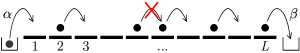
Figure 1: The TASEP with open boundary conditions. Each of the $L$ cells can be empty or occupied by one particle. If a specific occupied site is chosen to be updated, the particle can jump forward iff the next site is empty. For the case of open boundary conditions, particles can enter the system at site 1 with probability $\alpha$ and exit the system with probability $\beta$ at site $L$. For the case of periodic boundary conditions (not shown), site $L+1$ is identified with site 1 and the system becomes effectively a ring.

The TASEP is well-suited for an extension to networks. Its stationary state on a one-dimensional chain is known exactly both for periodic boundary conditions and open boundary conditions Schütz and Domany (1993); Derrida et al. (1993); Blythe and Evans (2007). In the steady state the average density profile $\rho(i)$ does not change with time. The current-density relation is given by

$$J(i)=\rho(i)(1-\rho(i+1)),$$ (1)

with $J(i)$ and $\rho(i)$ being the current and the density at site $i$, respectively. In the steady state, for a single TASEP segment the current is independent of the site, $J(i)=J$. For periodic boundary conditions, the steady state of the TASEP is given by a flat density profile, i.e. the density is site-independent with $\rho(i)=\rho=M/L$, $M$ being the total number of particles in the system. The current is given by $J=\rho(1-\rho)$ respectively. For the open boundary case, the system is also solved exactly. Here, the density is not site independent while the current still is, as a consequence of the continuity equation. The phase, a TASEP with open boundary conditions will be in, depends on $\alpha$ and $\beta$. For $L\rightarrow\infty$, the exact bulk densities $\rho_{\text{bulk}}=\rho(L/2)$ for the different phases are given by (see e.g. Schütz and Domany (1993); Derrida et al. (1993))

$$\rho_{\text{bulk}}(\alpha,\beta)=\begin{cases}\rho_{\text{LD}}=\alpha&{\rm for\ }\alpha<\beta,\alpha<1/2\\ \rho_{\text{HD}}=1-\beta&{\rm for\ }\beta<\alpha,\beta<1/2\\ \rho_{\text{MC}}=1/2&{\rm for\ }\alpha,\beta>1/2\\ \rho_{\text{DW}}=1/2&{\rm for\ }\alpha=\beta<1/2\end{cases}.$$ (2)

with specific deviations near the boundaries in each phase Schütz and Domany (1993); Derrida et al. (1993). Note that these deviations become larger, for smaller $L$. The subscript LD denotes the low density phase, HD the high density phase, MC the maximum current phase and DW the coexistence phase or domain wall phase. This DW phase is characterized by the diffusion of a domain wall which separates a low density region on the left and a high density region on the right. When measured over a long time, the averaged density profile becomes time-independent and is given by a linear ascent from $\alpha$ to $1-\alpha$.

For open boundary conditions the current $J$ also depends on the entrance and exit probabilities:

$$J(\alpha,\beta)=\begin{cases}\alpha(1-\alpha)&{\rm for\ }\alpha<\beta,\alpha<1/2\\ \beta(1-\beta)&{\rm for\ }\beta<\alpha,\beta<1/2\\ 1/4&{\rm for\ }\alpha,\beta>1/2\end{cases}.$$ (3)

These exact results for the one-dimensional chain can be used for an approximate description of TASEP network dynamics.

II.1.1 Traveltimes

Most research on the TASEP focusses on macroscopic observables like the current $J$ or the density $\rho$ while little attention has been given to the traveltime $T$. The traveltime is defined as the number of timesteps a particle needs to traverse the lattice, i.e. the time from entering site 1 until leaving site $L$. Since the stationary density profile is flat for periodic boundary conditions, in this case the traveltime can be calculated exactly as

$$T_{\text{PBC}}(\rho)=\frac{L}{1-\rho}.$$ (4)

For this, the average velocity $v=J/\rho$ was used. Note that the traveltime is a nonlinear function of the density in contrast to what is usually assumed in most studies of Braess paradox. For the case of open boundary conditions, exact traveltimes can in principle be calculated from the exact density profiles including the exact boundary behaviour. Eq. (4) holds pretty well for open boundary conditions when substituting the density by the exact bulk density $\rho=\rho_{\text{bulk}}$ of the system given by Eq. (2). From Fig. 2 we see that Eq. (4) (with $\rho=\rho_{\text{bulk}}$) shows notable deviations from the MC data only near the phase boundaries and especially in the domain wall phase (i.e. the phase boundary between HD and LD phases).

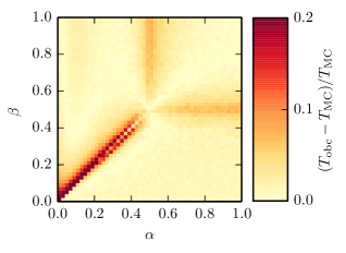
Figure 2: The relative difference of MC data from the approximative traveltimes (5) for open boundary conditions and system size $L=100$.

The latter are an effect of the fluctuations of the domain wall position in that phase. The deviations could be minimized by measuring over a really long time interval. However, really long measurement intervals $[t,t+\Delta t]$ are not suitable in our case since we want to simulate the situation of cars in a real road network where the effects for single drivers are relevant and not the $\Delta t\rightarrow\infty$ behaviour of the system. In this scenario, traveltimes of individual particles, each traversing the system at a different time and thus a different position of the domain wall and a different length of the HD region, will depend strongly on the explicit time of measurement and thus fluctuate from run to run.

Summarizing, we conclude that a TASEP with open boundary conditions shows a traveltime

$$T_{\text{OBC}}(\alpha,\beta)\approx T_{\text{PBC}}(\rho_{\text{bulk}}(\alpha,\beta))$$ (5)

with notable deviations only near the phase boundaries. The nonlinearity of the traveltimes combined with the microscopic exclusion principle and the stochasticity of the dynamics sets this model apart from models previously considered in the context of the Braess paradox. To our knowledge, so far only macroscopic models with linear traveltimes have been studied although there are indications for the paradox’s occurrence in the nonlinear case A Nagurney (2010).

II.2 TASEPs on networks

Most transport processes are not limited to a single segment. Transport takes place on networks where different routes between origin and destination are possible. This is obviously the case for road traffic in cities and also for freeways. The extension of the single TASEP to networks of TASEPs has been given a lot of attention in recent years. Networks of TASEPs are generally not exactly solvable. Due to this, mean field (MF) methods and MC studies are the tools to tackle these problems. The results obtained for the single-link versions of the TASEP model can be used as a good starting point to understand networks of TASEPs.

Over the years, different simple network topologies have been studied. For the case of random sequential updates, among others, the cases of one TASEP splitting into two lanes, then merging into one again Brankov et al. (2004), two TASEPs feeding into one Pronina and Kolomeisky (2005) and all different variations of four TASEPs B. Embley et al. (2009) (i.e. 3 on 1, 2 on 2, 1 on 3) were studied. Most of these cases focussed on open boundary conditions for the whole network while also some networks with constant global density were studied B. Embley et al. (2009). Beyond these simple topologies, three general network classes, Bethe networks, Poissonian networks and strongly correlated networks, have been examined I. Neri et al. (2011). Networks with parallel update schemes instead of the random sequential updates were examined in Wang et al. (2008); Liu and Wang (2009); Song et al. (2011). For brief summaries of most of the results obtained so far, see e.g. Ming-Zhe et al. (2012); Neri et al. (2013b).

When studying networks it has proven most useful to explicitly introduce so-called junction sites connecting the individual TASEPs which form the edges of the network B. Embley et al. (2009). MF treatment of networks neglects correlations between junction sites and the neighbouring start-/endpoints of the edges. This corresponds to treating all edges independently and neglecting inter-edge correlations. The edges $E_{i}$ can then be treated as single TASEPs with effective entrance and exit rates $\alpha^{\text{eff}}_{i}$, $\beta^{\text{eff}}_{i}$. These effective rates are then determined by the adjacent junction occupations. As an example consider edge $E_{A}$ being fed by junction $j_{m}$ with probability $p_{m,A}$ and exiting into junction $j_{n}$. Its effective rates are then $\alpha^{\text{eff}}_{A}=p_{m,A}\rho(j_{m})$ and $\beta^{\text{eff}}_{A}=1-\rho(j_{n})$. The current in this segment is then given by Eq. (3) as $J_{A}=J(\alpha^{\text{eff}}_{A},\beta^{\text{eff}}_{A})$. To solve the MF theory for the stationary state of a whole network, one has then to solve the coupled particle-conservation equations for all junctions which state that the density of a junction changes according to its incoming minus its outgoing currents. In the stationary state this change has to vanish. For most networks, this system of equations can only be solved numerically. When the effective rates are known, also the traveltimes of paths through a network can be approximated by Eq. (5). Here one has to keep in mind that the deviations from the bulk densities near the boundaries on network edges have a different form than on single TASEP segments due to the inter-link correlations. The deviations are in general larger than for single TASEPs (see e.g. Y. Baek et al. (2014) for an analysis of the behaviour near the boundaries) which is why the deviations from Eq. (5) are also larger. Still, Eq. (5) is a good approximation of how traveltimes on network edges scale with their (bulk-) densities.

II.2.1 The unbiased figure of eight network

Here we present the main results for a special case, the so-called unbiased figure of eight network as shown in Fig. 3. For a more detailed treatment, see B. Embley et al. (2009). The unbiased figure of eight network consists of two TASEPs $E_{A}$ and $E_{B}$, which feed and are – unbiasedly, i.e. with equal probability – fed by junction $j$.

Figure 3: The figure of eight network consists of two symmetric TASEPs $E_{A}$ and $E_{B}$ which feed onto and are, with probabilities $p_{A}$ and $p_{B}=1-p_{A}$, fed by junction $j$. In the unbiased case the probabilities are equal, $p_{A}=p_{B}=0.5$.

Due to the symmetry, both edges are always in the same state. This is either a LD, HD or domain wall state. A MC phase can not be reached since the effective entrance rates are always smaller than $1/2$ due to the unbiased feeding. Using this symmetry, in a mean-field picture, the particle density of the junction $\rho_{j}$ depends on the global density $\rho_{\text{global}}$ as

$$\rho_{j}=\begin{cases}2\rho_{\text{global}}&(\rho_{\text{global}}<1/3)\\ 2/3&(1/3<\rho_{\text{global}}<2/3)\\ \rho_{\text{global}}&(\rho_{\text{global}}>2/3)\end{cases}$$ (6)

and the current through the junction is given by

$$J=\begin{cases}2\rho_{\text{global}}(1-\rho_{\text{global}})&(\rho_{\text{global}}<1/3)\\ 2\cdot 2/9&(1/3<\rho_{\text{global}}<2/3)\\ 2\rho_{\text{global}}(1-\rho_{\text{global}})&(\rho_{\text{global}}>2/3)\end{cases}$$ (7)

as shown in Fig. 4.

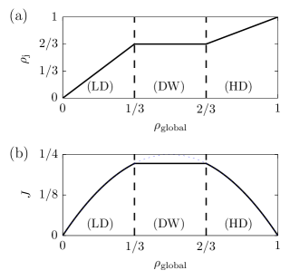
Figure 4: The unbiased figure of eight network shows a domain wall phase in a large intermediate density regime $1/3<\rho_{\text{global}}<2/3$. This can be seen in (a) the junction occupation $\rho_{j}$ which takes a constant value of 2/3 in that regime according to Eq. (6). As seen in (b) the current density relation shows that behaviour aswell, as the parabola for a single periodic TASEP $J=\rho(1-\rho)$ is truncated with constant value 2/9 in the DW regime according to Eq. (7).

This has an easily understandable interpretation. For low global densities ($\rho_{\text{global}}<1/3$), both segments are in a LD phase, while the density increases with the global density. At $\rho_{\text{global}}=1/3$, the effective rates of the edges become equal $\alpha^{\text{eff}}_{A/B}=\beta^{\text{eff}}_{A/B}=1/3$ which leads to diffusing domain walls between LD and forming HD segments in both links. The junction occupation saturates at $\rho_{j}=2/3$, while the lengths of the HD regions grow with growing global density. At $\rho_{\text{global}}=2/3$, the HD regions fill the whole edges. This behaviour is very different to single TASEPs. In single TASEPs with open boundary conditions domain walls only appear for fine tuned parameters $\alpha=\beta<1/2$, while in this network, they dominate the system over a large density regime ($1/3<\rho_{\text{global}}<2/3$) and are thus far more important for its analysis. It has indeed been shown that all regular networks are largely dominated by domain walls I. Neri et al. (2011).

The biased version of the figure of eight network where the probabilites for jumps from the junction to the edges are different (Fig. 3) shows two plateaus in the fundamental diagram, corresponding to domain wall phases, for two distinct global density regimes. For more details see B. Embley et al. (2009). This study has also been extended to symmetric junctions feeding onto more than two edges I. Neri et al. (2011); Y. Baek et al. (2014).

We have repeated the specific results for the unbiased figure of eight here, since they correspond to a special case of our network as discussed in Sec. III.1.

II.3 Periodic Braess network

We now examine the network structure, originally proposed by Braess D. Braess (1968); D. Braess et al. (2005), shown in Fig. 5. The individual edges $E_{1},\ldots,E_{5}$ are made up by TASEPs joined by junction sites $j_{1},\ldots,j_{4}$. We examine the traveltimes from start (junction $j_{1}$) to finish (junction $j_{4}$). Periodic boundary conditions are achieved by coupling $j_{4}$ with $j_{1}$ via an additional TASEP $E_{0}$ of length $L_{0}=1$. Like this, the total number of particles $M$ in the system and thus the global density $\rho_{\text{global}}=M/(4+\sum^{5}_{i=0}L_{i})$ are constant. Note that due to the random-sequential update there cannot be conflicts like two particles attempting to jump onto a junction site (like e.g. from the ends of $E_{5}$ and $E_{2}$ onto $j_{3}$).

Figure 5: The network, as proposed by Braess D. Braess (1968); D. Braess et al. (2005), that is studied throughout this paper. Different to the original network we are considering periodic boundary conditions implemented by the link $E_{0}$. All links are realized by TASEPs.

Edge $E_{5}$ is considered the additional edge which is supposed to be added to the system. The network is always chosen to be symmetric with

$$L_{1}=L_{3}\qquad\text{and}\qquad L_{2}=L_{4}\,.$$ (8)

We consider the case $L_{1}\leq L_{2}$. Thus, for

$$L_{5}\leq L_{2}-L_{1}-1$$ (9)

the addition of $E_{5}$ results in a new possible route through the system, which is of shorter or equal length as the routes without the new link:

$$\hat{L}_{153} = 5+L_{1}+L_{3}+L_{5}$$ (10)

$$\leq 4+L_{1}+L_{2}$$

$$= \hat{L}_{14}=\hat{L}_{23},$$ (11)

with $\hat{L}_{i}$ denoting lengths of routes. On junctions $j_{1}$ and $j_{2}$, the particles turn left with probabilities $\gamma$ and $\delta$ and right with probabilites $1-\gamma$ and $1-\delta$. For the reminder of this paper, the system with (without) $E_{5}$ is also denoted as 5link (4link) or with the superscript 5 (4), respectively. We will use the global densities of the system with $E_{5}$ and without $E_{5}$ when comparing the two systems. Both densities are related through $M$ as follows:

$$\rho^{(5)}_{\text{global}} = \rho^{(4)}_{\text{global}}\frac{5+2L_{1}+2L_{2}}{5+2L_{1}+2L_{2}+L_{5}}$$ (12)

$$= \rho^{(4)}_{\text{global}}\frac{5+2L_{1}+2L_{2}}{2L_{2}+\frac{\hat{L}_{153}}{\hat{L}_{14}}(4+L_{1}+L_{2})}.$$

The latter equality will be used when we present the phase diagram in Sec. III.3. In our further analysis we will compare the traveltimes of different routes through the system denoted by $T_{i}$. The traveltime $T_{153}$ of route 153 is then the number of timesteps a particle sitting on $j_{1}$ needs until it jumps out of $j_{4}$ if it traverses the system via $E_{1}$, $j_{2}$, $E_{5}$, $j_{3}$, $E_{3}$. The traveltimes $T_{14}$, $T_{23}$ of the two other possible routes are defined respectively.

II.3.1 User optimum and system optimum

To determine how the new link $E_{5}$ effects the network performance in the sense of expected traveltimes, one needs to find the new stationary state of the system. A specific demand, given by $\rho^{(5)}_{\text{global}}$, will result in a specific distribution of the particles onto the three possible paths. Without traffic regulations and with complete knowledge about expected traveltimes, selfishly deciding drivers will choose their route through the system such that they minimize their individual traveltimes. This results in a stable state, the so-called user optimum (Nash equilibrium) of the system. The user optimum ($uo$) is given by the demand distribution that leads to equal traveltimes on all three possible routes through the system. This state is stable since it would not make sense for drivers to redecide for a different route if all routes have the same traveltime and route changes would increase the traveltime. Special cases are given if one or two routes are not used at all and have a higher traveltime than the other used routes. One example for such a special state would be an ”all 153” state. This state can occur for specific demands if all particles use route 153 and nevertheless the traveltime on this route is lower then on the unused routes 14 and 23. This distribution would then be the user optimum if there is no other distribution of the particles that leads to equal and lower traveltimes on all three routes.

The other significant state is the system optimum ($so$) given by the demand distribution which minimizes the maximum of the traveltimes on the three routes through the system. Note that throughout the literature there are different definitions of the system optimum. Sometimes it is also defined as the state that minimizes the total traveltime, i.e. the sum of all traveltimes Thunig and Nagel (2016). Here we follow Braess D. Braess (1968); D. Braess et al. (2005) who used the definition based on the minimization of the maximum traveltime. Furthermore the specific choice is not as important since eventually we compare the traveltimes of the user optima with and without the new link to deduce how the new link effects the system. For our investigation the system optima are not really crucial. However, we will later use them to distinguish different Braess phases (see Sec. II.3.3). By our definition, the maximum traveltime $T_{\text{max}}(so)$ in the system optimum is always shorter than or equal to the traveltimes $T(uo)$ in the user optimum. This means that for the whole system and all individual drivers, in terms of traveltimes the system optimum is always better than or equal to the user optimum. Since the traveltimes on the three routes can be different in the system optimum state it is not expected to be stable if drivers decide selfishly. Drivers on a route with a higher traveltime will redecide for a route with lower traveltime thus leading to a different demand distribution. Without traffic regulations, the system’s new stationary stable state will be the user optimum.

One expects that, because of symmetry, without $E_{5}$ the system optimum is always equal to the user optimum at $\gamma=0.5$. With $E_{5}$, the user optimum can be different from the system optimum. The Braess paradox in its original sense is the case that $T(uo)$ with $E_{5}$ is larger than $T(uo)$ without $E_{5}$, meaning that the addition of the new route leads to a user optimum with higher traveltimes than the user optimum without $E_{5}$.

II.3.2 Observables

In our simulations the demand distributions are determined by the turning probabilities $\gamma$ and $\delta$. In the following a pair $(\gamma,\delta)$, corresponding to a specific demand distribution, will be called a strategy. By varying $\gamma,\delta\in[0,1]$ we realize all possible strategies. To analyse for which values of $\gamma$ and $\delta$ the system is in its system optimum or user optimum state, we define two observables:

$$\Delta T = |T_{14}-T_{23}|+|T_{14}-T_{153}|+|T_{23}-T_{153}|$$ (13)

$$T_{\text{max}} = \text{max}[T_{i},i\in\{14,23,153\}].$$ (14)

Analysing these observables for all possible pairs $(\gamma,\delta)$, we can use them to infer the strategies that correspond to the user optimum and the system optimum as:

• $uo$ given by $(\gamma,\delta)_{uo}$ fulfilling $\Delta T=0$

• $so$ given by $(\gamma,\delta)_{so}$ minimizing $T_{\text{max}}$.

This is because the strategy $uo=(\gamma,\delta)_{uo}$ fulfilling $\Delta T=0$ leads to equal traveltimes on all routes according to (13). Due to numerical limitations and fluctuations in the simulations the case of an exact equality is often not found, which is why we identify the strategy corresponding to the minimium of $\Delta T$ with the user optimum. Furthermore, for $\Delta T$ there are some special cases: If e.g. only one route is used and has a lower traveltime than the unused routes, this is defined as $\Delta T=0$, since such a state corresponds to the user optimum as discussed in the previous subchapter. This can only arise for the cases $\{\gamma=0\lor\gamma=1\}\lor\{(0<\gamma<1)\land(\delta=0\lor\delta=1)\}$. The strategy $so=(\gamma,\delta)_{so}$ corresponds to the state where the longest of the three traveltimes is minimal compared to the other strategies.

II.3.3 Classification of system states

Assuming that both the user optimum and the system optimum are clearly identifiable, there is a limited number of possibilities for system states. By ”clearly identifiable” we mean that all three routes have stable traveltimes and there is a distinct minimum for $T_{\text{max}}$ and a distinct minimum for $\Delta T$ with a value close to zero. In the next section we will see that this is not always the case, since depending on $\rho_{\text{global}}$ and $\gamma$ and $\delta$, routes or parts of routes can be in domain wall phases leading to strongly fluctuating traveltimes. In this case there are no stable traveltime landscapes and no clearly identifiable system or user optima.

We now focus on the case where system optimum and user optimum are clearly identifiable. This allows us to make a prediction about the phases that can be observed in the system. The possible states are shown in Fig. 6.

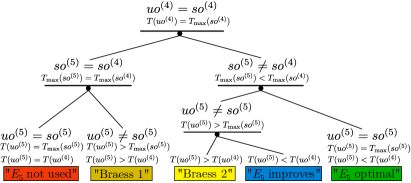
Figure 6: Tree of the possible system states, if user optimum $uo$ and system optimum $so$ are clearly identifiable. The superscript $(4)$ stands for the system without $E_{5}$, while the superscript $(5)$ denotes the system with $E_{5}$.

If there are stable values for traveltimes and no traffic regulations, we can build the tree of possible states from the starting point of $uo^{(4)}=so^{(4)}$, which is expected to be always true due to symmetry. From here, we can compare $so^{(5)}$ and $so^{(4)}$.

If $so^{(5)}=so^{(4)}$, the additional link cannot lead to a stable state with lower traveltimes. If in this case $uo^{(5)}=so^{(5)}$, the system will end up in a state with $E_{5}$ not being used at all (”$E_{5}$ not used”). If $uo^{(5)}\neq so^{(5)}$, the system will actually be in a stable state with higher traveltimes than the system without $E_{5}$ since in this case $T(uo^{(5)})>T(uo^{(4)})$. This is the classical Braess case, named ”Braess 1” in this paper.

For the case $so^{(5)}\neq so^{(4)}$ the system can potentially be improved (w.r.t. traveltimes) through the addition of $E_{5}$ since in this case $T_{\text{max}}(so^{(5)})\leq T_{\text{max}}(so^{(4)})$ has to be true. If in the 5link system $uo^{(5)}=so^{(5)}$, the system will be in its optimal state, which has lower traveltimes than the stable state of the 4link system. This is denoted as ”$E_{5}$ optimal”. In the case of $uo^{(5)}\neq so^{(5)}$, the 5link system will not be in its optimal state. Two cases can be distinguished. If $T(uo^{(5)})>T(uo^{(4)})$, called ”Braess 2”, the system will be in a state with higher traveltimes than the 4link. If $T(uo^{(5)})<T(uo^{(4)})$, called ”$E_{5}$ improves”, the system will be in a state with lower traveltimes than the 4link but still with higher traveltimes than the system optimum of the 5link.

According to these possible states and additional results from the following chapters, we will present a phase diagram of the system in Sec. III.3.

III Results

First we show a mixed MF and MC study of the system without the new road at $\gamma=0.5$. From that we can already see that, at intermediate densities, we are not able to find stable system or user optima since parts of the system are in domain wall phases leading to strongly fluctuating traveltimes. In the next subsection we present the results of MC simulations of the system with the new link.

III.1 Symmetric system without the new edge

Here we study the system without link $E_{5}$. Due to symmetry, one would expect that for all values of $\rho^{(4)}_{\text{global}}$ the user optimum and the system optimum were given for $\gamma=0.5$. One expects that if on average half of the particles choose route 14 and the other half route 23, this would lead to equal traveltimes and thus also minimize the maximum traveltime. While this symmetry argument appears to be obvious, it turns out that it is not true for all densities $\rho^{(4)}_{\text{global}}$ in the sense that there are no stable traveltimes in the system in a large intermediate global density regime. Thus we find that we cannot use the straightforward traveltime analysis and therefore cannot find user optima and/or system optima in this density regime. Here we show why this is the case.

As seen in Fig. 7, without the new link, at $\gamma=0.5$ the Braess network becomes approximately equal to the unbiased figure of eight network. This network was studied in B. Embley et al. (2009) and the main results were summarized in Sec. II.2.1. The only difference is that in our case the two edges, now given by paths 14 and 23, feed into junction $j_{4}$ and are fed by junction $j_{1}$ while going from $j_{4}$ to $j_{1}$ via $E_{0}$ (of length $L_{0}=1$).

Figure 7: Without $E_{5}$ and with $\gamma=0.5$ the periodic Braess network comes very close to the unbiased figure of eight network studied in chapter II.2.1 (for details see B. Embley et al. (2009)). The only difference is that in our case, the two paths are connected via three sites while in B. Embley et al. (2009) only one junction site connects the two paths.

Thus there are three sites connecting inputs and outputs instead of just one junction $j$ in the original figure of eight network (see Fig. 3). While the MF arguments for the derivation B. Embley et al. (2009) of the main results on the figure of eight network, given by Eqs. (6) and (7), do not hold exactly in our case, the system behaves similarly. To visualize this, in Fig. 8 MC measurements of the effective entrance and exit rates of paths 14 and 23 are shown.

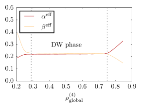
Figure 8: The MC effective entrance ($\alpha^{\text{eff}}$) and exit ($\beta^{\text{eff}}$) rates of paths 14 and 23 for the system without $E_{5}$ and $\gamma=0.5$. In the region of $0.29\lesssim\rho^{\text{(4)}}_{\text{global}}\lesssim 0.75$ they are roughly equal and the paths will be in the domain wall phase. They were obtained from MC measurements of $\rho(j_{1})$ and $\rho(j_{4})$ for a system of size $L_{0}=1$, $L_{1}=100$, $L_{2}=500$.

For $\gamma=0.5$ they have the same functional dependence for both paths and are given by

$$\alpha^{\text{eff}} = \frac{1}{2}\rho(j_{1}),$$ (15)

$$\beta^{\text{eff}} = 1-\rho(j_{4}).$$ (16)

One sees that their values are approximately equal for $0.29\lesssim\rho^{(4)}_{\text{global}}\lesssim 0.75$ and thus both paths are in domain wall phases in this large intermediate density regime. This region is even larger than in the former studied figure of eight network. This is due to the fact that the three connecting sites result in a larger effective bottleneck effect than just one junction site. The interpretation is the same as for the figure of eight network in Sec. II.2.1. For global densities $\rho^{(4)}_{\text{global}}\lesssim 0.29$, both paths are in LD states. In the whole intermediate density regime $0.29\lesssim\rho^{(4)}_{\text{global}}\lesssim 0.75$ both paths are in a DW state. With growing global density, the length of the HD regions grows compared to the LD regions. For $\rho^{(4)}_{\text{global}}\gtrsim 0.75$, both routes are in HD phases. In the DW phase we do not expect stable traveltimes since the position of the domain wall changes constantly. The HD regions queue behind the bottleneck (junction $j_{4}$), but the position of the domain wall is changing constantly. This means that the total length of the HD regions $L_{HD}$ is constant, but the distribution of this region onto the two paths changes. All states between the whole HD region being in path 14 to the whole HD region being in path 23 are accessible. The densities of the LD and HD regions in the domain wall phase are given by

$$\rho_{\text{LD}} \approx \alpha^{\text{eff}}$$ (17)

$$\rho_{\text{HD}} \approx 1-\alpha^{\text{eff}}.$$ (18)

From the measurements shown in Fig. 8 we deduce that in the whole domain wall phase, $\alpha^{\text{eff}}\approx\beta^{\text{eff}}\approx 0.22$. From this we can now calculate the maximum and minimum traveltimes which can be measured on both routes. To do this, first note that the following two equations have to be valid:

$$M=\rho^{(4)}_{\text{global}}L^{(4)}_{\text{tot}} \approx \rho_{\text{HD}}L_{\text{HD}}+\rho_{\text{LD}}L_{\text{LD}}\,,$$ (19)

$$L^{(4)}_{\text{tot}} \approx L_{\text{HD}}+L_{\text{LD}}.$$ (20)

These are not exact equalities but approximations since sharp discontinous domain walls separating the LD and HD regions were assumed. Furthermore we neglected the junction sites and the site of $E_{0}$ to approximate the total number of sites in the system without $E_{5}$ as $L^{(4)}_{\text{tot}}=2L_{1}+2L_{2}+5\approx 2L_{1}+2L_{2}$. Using $\rho_{\text{LD}}\approx 1-\rho_{\text{HD}}$ from Eqs. (17) and (18), the system of Eqs. (19) and (20) can be solved:

$$L_{\text{HD}}=\frac{\rho^{(4)}_{\text{global}}L^{(4)}_{\text{tot}}}{\rho_{\text{HD}}-\rho_{\text{LD}}}-\frac{\rho_{\text{LD}}L^{(4)}_{\text{tot}}}{\rho_{\text{HD}}-\rho_{\text{LD}}}.$$ (21)

This equation tells us how long the HD region is depending on the global density. If we now make a further approximation and assume that the LD and HD regions themselves have flat density profiles with a sharp domain wall separating them, we can assume that Eq. (5), $T_{\text{OBC}}\approx L/(1-\rho_{\text{bulk}}(\alpha,\beta))$, holds approximately for the description of the traveltime on the LD and HD parts of the paths. Using these assumptions we can then deduce the minimum and maximum possible traveltimes of routes 14 and 23 in the DW phase:

$$T_{\text{max}}\approx\begin{cases}\frac{L_{\text{HD}}}{1-\rho_{\text{HD}}}+\frac{\hat{L}_{14}-L_{\text{HD}}}{1-\rho_{\text{LD}}}&L_{\text{HD}}<\hat{L}_{14}\\ \frac{\hat{L}_{14}}{1-\rho_{\text{HD}}}&L_{\text{HD}}>\hat{L}_{14}\end{cases},$$ (22)

$$T_{\text{min}}\approx\begin{cases}\frac{\hat{L}_{14}}{1-\rho_{\text{LD}}}&L_{\text{HD}}<\hat{L}_{14}\\ \frac{L_{\text{HD}}-\hat{L}_{14}}{1-\rho_{\text{HD}}}+\frac{L_{\text{LD}}}{1-\rho_{\text{LD}}}&L_{\text{HD}}>\hat{L}_{14}\end{cases}.$$ (23)

For the case where the whole HD segment is shorter than a route ($L_{\text{HD}}<\hat{L}_{14}$), the maximum traveltime is always given if the whole HD segment is inside one route only. This leads to the minimal traveltime on the other route since the other route is completely in an LD phase. The situation changes as the HD region gets longer than a whole route, $L_{\text{HD}}>\hat{L}_{14}$. Then the maximum traveltime is realized if a whole route is in a HD state which realizes the minimum traveltime the other route where the ’remnant’ of the HD segment is. These two different situations are shown in Fig. 9.

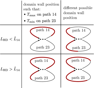
Figure 9: Schematic of the possible domain wall positions. For $L_{\text{HD}}<\hat{L}_{14}$ (upper row), the maximum/minimum traveltimes can be measured on path 14/23 if the whole HD region (marked red) is on path 14 (left column). For $L_{\text{HD}}>\hat{L}_{14}$ (lower row), the maximum/minimum traveltimes can be measured on path 14/23 if a whole path is in the HD phase, while the remnant of the HD region is in the other path (left column). The right column shows two possible different domain wall positions for the same $L_{\text{HD}}$ that occur at different measurement times.

This behavior and the approximative Eqs. (22) and (23) were confirmed by MC measurements as shown in Fig. 10.

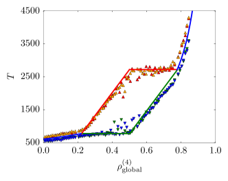
Figure 10: The minimum and maximum traveltimes of the system without $E_{5}$ for $L_{1}=100$, $L_{2}=500$. In the large intermediate DW phase, Eq. (22) and (23) are good approximations for the maximum (red line) and minimum (green line) traveltimes. Outside of the DW phase, Eq. (5) (blue lines) is a good approximation for the traveltimes. The equations show a good agreement with MC data (red/orange $\vartriangle$ for $T_{\text{max},14/23}$, green/blue $\triangledown$ for $T_{\text{min},14/23}$). For each global density $\rho^{(4)}_{\text{global}}$ the traveltimes of each path were measured 400 times and the minimum and maximum values are plotted.

Eqs. (22) and (23) give a very good approximation for the minimum and maximum traveltimes in the DW phase. For the pure LD and HD phases we just assumed flat density profiles and one stable traveltime value, approximately described by Eq. (5). MC measurements confirm the expected behaviour. For each global density we made 400 individual measurements for the traveltimes of routes 14 and 23. Then we plotted the minimum and maximum values. The expected behaviour of a stable traveltime value in the LD and HD regime as well as the approximate expressions (23) and (22) are confirmed.

To further clarify the effects of the fluctuating domain wall in the DW phase we collected and binned the traveltimes of 400 individual measurements of the traveltimes of routes 14 and 23 (traveltimes for route 153 are included for completeness). The histograms are shown in Fig. 11 for three different global densities, $\rho^{(4)}_{\text{global}}\in\{0.2,0.5,0.85\}$.

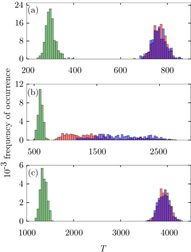
Figure 11: Histograms of the traveltime measurements in the system of size $L_{0}=1$, $L_{1}=100$, $L_{2}=500$, $L_{5}=37$ for $\gamma=0.5$ and $\delta=1.0$ and (a) $\rho^{(4)}_{\text{global}}=0.2$, (b) $\rho^{(4)}_{\text{global}}=0.5$, (c) $\rho^{(4)}_{\text{global}}=0.85$. The red bars represent the traveltimes on path 14, the blue bars those of path 23 and the green bars those of path 153. One can see that for the intermediate density, there is no well defined maximum in the traveltime distributions of paths 14 and 23, since these paths are in the domain wall phase. For each path 400 measurements were performed and binned.

We find that there is a well-defined mean in the LD and HD regions but not in the DW region ($\rho^{(4)}_{\text{global}}=0.5$). Here all the accessible traveltimes between $T_{\text{min}}$ and $T_{\text{max}}$ are observed with approximately the same frequency of occurrence.

The findings of these combined MF and MC arguments show that (for finite measurement intervals) in the large intermediate density regime there are no stable expectation values for the traveltimes of the routes in the system, even though the system is in a nonequilibrium stationary state. Thus it is not possible to identify the system and user optima in this density region in the straightforward way described in Sec. II.3.2. It turns out that the system with $E_{5}$ is also dominated by domain walls in an even larger density regime. Thus, with the means of traveltime measurements, we can only identify the user and system optima of the system outside of these densities.

III.2 Characterization of the phases

Here we present the results of our MC simulations of the whole system with $E_{5}$. The MC data were gathered as follows. The system was always initialized randomly. Then, for given values of $(\gamma,\delta)$, the system was relaxed/propagated for at least $2\cdot 10^{5}$ sweeps. To measure traveltimes for the three paths through the system, a particle was tracked on junction $j_{1}$ and then ”manually navigated” through the current path. During this time the rest of the system was still propagated according to $\gamma$ and $\delta$. In detail this was done as follows: To determine e.g. a traveltime value for path 153, after relaxation, a particle sitting on $j_{1}$ is tagged. Since we want to measure $T_{153}$, it is then forced to jump to $E_{1}$, no matter the value of $\gamma$. If the tagged particle arrives on $j_{2}$, it is then forced to jump to $E_{5}$ and once it reaches $j_{3}$ to $E_{3}$. Once it reaches $j_{4}$, the timesteps for the whole way to get there from $j_{1}$ give one measurement value for $T_{153}$. During this measurement the rest of the system (all other particles) keeps evolving according to $(\gamma,\delta)$. At least 200 individual times were measured for each path and the mean and standard deviation were obtained. From these measurements, the values of $\Delta T$ and $T_{\text{max}}$ were calculated. The parameter region $\gamma,\delta\in[0.0,1.0]$ was sweeped in steps of 0.1. It should be noted that like this the positions of the system optima and user optima can only be found roughly and that the exact positions may lie between the points of the 0.1 grid. Despite the relatively large stepwidth of 0.1 we are still able to conclude whether system optimum and user optimum are in the same region. This is sufficient to deduce the phase of the system for the given parameters. We analysed the traveltimes for different system parameters like length ratios and densities and found that the relevant parameters are the pathlength-ratio $\hat{L}_{153}/\hat{L}_{14}$ (note: $\hat{L}_{14}=\hat{L}_{23}$) and the global density $\rho_{\text{global}}$. In this section we present examples for how the $T_{\text{max}}$- and $\Delta T$-landscapes look like in the different phases and also show the density profiles of the paths in the system optima and user optima. After that, we present a phase diagram predicting the phase of the system dependent on the crucial parameters.

For low global densities we find stable traveltimes and definite minima of our observables and can thus deduce the system and user optima of the system. For intermediate densities, fluctuations dominate the system as already indicated in the previous section on the system without $E_{5}$. For high global densities we find stable results again but are not able to identify system and user optima in this straightforward approach.

III.2.1 Low global densities

For low global densities $\rho^{(4)}_{\text{global}}\lesssim 0.29$ (and the corresponding global densities $\rho^{(5)}_{\text{global}}$ given by Eq. (12)), we can find strategies $(\gamma,\delta)$ in the parameter space where $T_{\text{max}}$ and $\Delta T$ are minimized. This is possible since the fluctuations of the traveltimes of the paths $i$, quantifiably by the standard deviations $\sigma=\sqrt{\sum_{i}\frac{(\bar{T}-T_{i})^{2}}{N}}$, are small and the traveltimes have stable values. In the low density regime, for most strategies all links of the network are in LD, HD or MC phases.

In Fig. 12 an example for ”$E_{5}$ optimal” case is shown. This is a special ”all 153” case of that phase since here both $T_{\text{max}}$ and $\Delta T$ have their minima at $(\gamma,\delta)_{uo}=(\gamma,\delta)_{so}=(1.0,0.0)$, meaning that the stable state is achieved when all particles choose path 153. Thus this is the only used path.

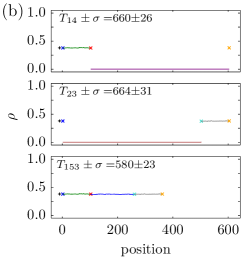
Figure 12: An example for the ”$E_{5}$ optimal” (”all 153”) case. Parameters are $L_{0}=1$, $L_{1}=100$, $L_{2}=500$, $L_{5}=157$, $M=136$. This means $\hat{L}_{153}/\hat{L}_{14}\approx 0.6$, $\rho^{(5)}_{\text{global}}\approx 0.1$. (a) $T_{\text{max}}$- and $\Delta T$-landscapes. The white asterisks indicate the system and user optimum, respectively. (b) Density profiles and average traveltimes of the three paths for $\text{min}(T_{\text{max}})$ and $\text{min}(\Delta T)$ - both at $\gamma=1.0$, $\delta=0.0$.

Fig. 13 shows an example of ”$E_{5}$ optimal” case where not all particles choose path 153, but the stable state $(\gamma,\delta)_{uo}=(\gamma,\delta)_{so}$ develops at $(\gamma,\delta)\approx(0.8,0.3)$.

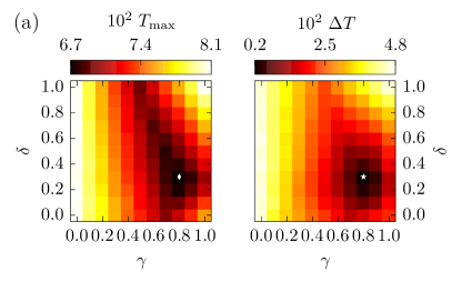
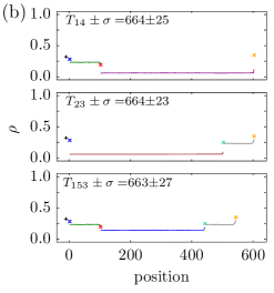
Figure 13: An example for the ”$E_{5}$ optimal” case. Parameters are $L_{0}=1$, $L_{1}=100$, $L_{2}=500$, $L_{5}=339$, $M=154$. This means $\hat{L}_{153}/\hat{L}_{14}\approx 0.9$, $\rho^{(5)}_{\text{global}}\approx 0.1$. (a) $T_{\text{max}}$- and $\Delta T$-landscapes. The white asterisks indicate the system and user optimum, respectively. (b) Density profiles and average traveltimes of the three paths for $\text{min}(T_{\text{max}})$ and $\text{min}(\Delta T)$ - both at $\gamma=0.8$, $\delta=0.3$.

In Fig. 14, an example of the ”Braess 1” phase is shown. The system optimum is at $(\gamma,\delta)_{so}=(0.5,1.0)$, thus at the 4link system optimum, meaning that in the system optimum $E_{5}$ is not used. The user optimum is found at $(\gamma,\delta)_{uo}\approx(0.8,0.6)$. Thus, without traffic regulations, a stable state will develop in that region resulting in higher traveltimes for all particles, than in the 4link system. In the density profiles shown in Fig. 14 we can see that not all paths are in perfect LD, HD or MC phases even in this low density regime and that the standard deviations of the traveltimes are higher (relatively, compared to the mean value) than in the ”$E_{5}$ optimal” cases. This suggests that domain walls are already present at these low global densities. We plan to investigate this point further in the future. Nevertheless, the fluctuations are still small enough to consider the system to be in a stable state at $(\gamma,\delta)_{uo}\approx(0.8,0.6)$.

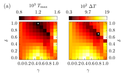
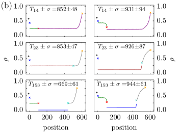
Figure 14: An example for the ”Braess 1” case. Parameters are $L_{0}=1$, $L_{1}=100$, $L_{2}=500$, $L_{5}=339$, $M=309$. This means $\hat{L}_{153}/\hat{L}_{14}\approx 0.9$, $\rho^{(5)}_{\text{global}}\approx 0.2$. (a) $T_{\text{max}}$- and $\Delta T$-landscapes. The white asterisks indicate the system and user optimum, respectively. (b) Density profiles and average traveltimes of the three paths for $\text{min}(T_{\text{max}})$ at $\gamma=0.5$, $\delta=1.0$ (left) and $\text{min}(\Delta T)$ at $\gamma=0.8$, $\delta=0.7$ (right).

III.2.2 Intermediate global densities

For intermediate global densities $0.29\lesssim\rho^{(4)}_{\text{global}}\lesssim 0.9$, fluctuations dominate the system with the new link for most strategies. This is an even larger density region than for the system without the new link. These fluctuations are due to links or whole routes of the system being in DW states, as explained in Sec. III.1. Fluctuations are highest for strategies close to the minima of $\Delta T$ and $T_{\text{max}}$. An example of the $\Delta T$ -and $T_{\text{max}}$-landscapes at intermediate global densities is shown in Fig. 15. The domain walls fingerprint can be found in the (almost) linear average density profiles. As explained before, the traveltimes fluctuate strongly and do not have a well-defined mean as shown in Fig. 11. Therefore the $\Delta T$ -and $T_{\text{max}}$-landscapes cannot be used to determine the system’s stable state and are thus somewhat meaningless. Nevertheless, in this whole density region the minima of $T_{\text{max}}$ were found at $(\gamma,\delta)=(0.5,1.0)$. This suggests that the addition of $E_{5}$ cannot lead to stable states with lower traveltimes for these demands. A more detailed characterization of this phase is another aim of future research. Here we just call this intermediate density regime the ”fluctuation-dominated phase”. Definite stable states cannot be found by the straighforward traveltime analysis.

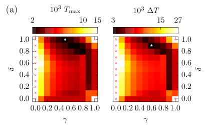
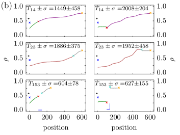
Figure 15: A state example from the fluctuation-dominated region. Parameters are $L_{0}=1$, $L_{1}=100$, $L_{2}=500$, $L_{5}=37$, $M=621$. This means $\hat{L}_{153}/\hat{L}_{14}\approx 0.4$, $\rho^{(5)}_{\text{global}}\approx 0.5$. (a) $T_{\text{max}}$- and $\Delta T$-landscapes. The white asterisks indicate the system and user optimum, respectively. Strategies marked by a red cross lead to gridlock states. (b) Density profiles and average traveltimes of the three paths for $\text{min}(T_{\text{max}})$ at $\gamma=0.5$, $\delta=1.0$ (left) and $\text{min}(\Delta T)$ at $\gamma=0.6$, $\delta=0.9$ (right).

In certain limits, e.g. for $\gamma\to 0$, the traveltime diverges due to the formation of gridlocks. In this case, on one of the routes all sites are occupied.

III.2.3 High global densities

For high densities, $\rho^{(4)}_{\text{global}}\gtrsim 0.9$, $E_{5}$ can lead to lower traveltimes in the system. This is easily explained by Eq. (4), showing a diverging traveltime for $\rho\rightarrow 1$. As seen in Fig. 16, the 5link system optimum moves away from the 4link system optimum. Also, as in the case of intermediate global densities, gridlocks can occur. It turns out that we cannot find a definite user optimum with $\text{min}(\Delta T)\rightarrow 0$ for these cases. We can deduce that $so^{(5)}\neq uo^{(5)}$ and the minimum of $\Delta T$ lies in a parameter region where the value of $T_{\text{max}}$ is smaller than at $(\gamma,\delta)=(0.5,1.0)$. This means that the system is in the ”$E_{5}$ improves” case according to Fig. 6.

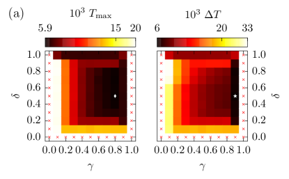
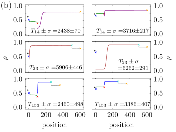
Figure 16: An example for the ”$E_{5}$ improves” case. Parameters are $L_{0}=1$, $L_{1}=100$, $L_{2}=500$, $L_{5}=157$, $M=1090$. This means $\hat{L}_{153}/\hat{L}_{14}\approx 0.6$, $\rho^{(5)}_{\text{global}}\approx 0.8$. (a) $T_{\text{max}}$- and $\Delta T$-landscapes. The white asterisks indicate the system and user optimum, respectively. Strategies marked by a red cross lead to gridlock states. (b) Density profiles and average traveltimes of the three paths for $\text{min}(T_{\text{max}})$ at $\gamma=0.8$, $\delta=0.5$ (left) and $\text{min}(\Delta T)$ at $\gamma=0.9$, $\delta=0.5$ (right).

For even higher densities $\rho^{(4)}_{\text{global}}\geq 1.0>\rho^{(5)}_{\text{global}}$, the 4link system is full and thus we cannot compare traveltimes of the 4link with the 5link for these densities. We deduce that, trivially, $E_{5}$ leads to lower traveltimes in these cases.

III.3 Phase diagram

In Fig. 17 we present a phase diagram showing the regimes defined in Fig. 6 as a function of the system parameters. In the presented phase diagram we used the length ratio $L_{1}/L_{2}=1/5$, limiting the pathlength ratios to $\hat{L}_{153}/\hat{L}_{14}\gtrsim 0.34$. The measurements were repeated for different values of that ratio and showed the same results. The only difference is that, in accordance with Eq. (9), different regions of $\hat{L}_{153}/\hat{L}_{14}$ are available. We also repeated the measurements for a ten times larger system $\tilde{L}_{i}=10L_{i}$, to be sure that we are not dealing with finite size effects. The larger system also yielded the same results. Data was gathered as follows: First the whole parameter region was sweeped in steps of 0.1. For each pair of $\hat{L}_{153}/\hat{L}_{14}$ and $\rho^{\text{(5)}}_{\text{global}}$ we analyzed the $T_{\text{max}}$ -and $\Delta T$-landscapes like in the examples in the previous section. After getting a rough idea of the phase landscape, the phase boundaries were determined with finer resolution.

We can see that for low densities and small pathlength ratios the system is in the ”$E_{5}$ optimal”/”all 153” phase, phase I, in the sense that all particles will use path 153 (thus $\gamma=1.0$ and $\delta=0.0$). The phase border of this phase can also be approximated analytically. Two conditions which can be approximated by two equations have to be valid for the system to be in the ”all 153” phase. Traveltime $T_{153}$ has to be lower than the other routes’ traveltimes $T_{14}$ and $T_{23}$. This happens if

$$T_{153}\approx\frac{\hat{L}_{153}}{1-\frac{M}{\hat{L}_{153}}}\lesssim T_{14}\approx T_{23}\approx\frac{L_{13}}{1-\frac{M}{\hat{L_{153}}}}+L_{24},$$ (24)

since all particles choose route 153. To make sure that in this case the traveltime $T_{153}$ is actually shorter than the traveltime of the user optimum of the system without $E_{5}$, the second condition

$$\frac{\hat{L}_{153}}{1-\frac{M}{\hat{L}_{153}}}\lesssim\frac{\hat{L}_{14}}{1-\frac{M}{2\hat{L}_{14}}}\approx\frac{\hat{L}_{23}}{1-\frac{M}{2\hat{L}_{23}}}$$ (25)

also has to hold if we assume that the stationary state of the 4link system will be reached if approximately half of the particles choose route 14 and the other half route 23. For both equations flat density profiles are assumed on the paths, which is why these equations are just approximations. The lines given by Eq. (24) (blue line) and (25) (magenta line) are shown in Fig. 17. The two conditions are fulfilled in the regions of the phase diagram below both lines. This behaviour is confirmed very well by our simulations which confirm the system to be in an ”all 153” state (MC-data symbols $\triangleleft$) in that region.

For larger pathlength ratios, there will also be a region where a stable state in the ”$E_{5}$ optimal” phase develops in which all paths are used (phase II). For larger densities up to $\rho^{\text{(4)}}_{\text{global}}\approx 0.29$, the system is in the ”Braess 1” phase (phase III). Above that, for densities $0.29\lesssim\rho^{\text{(4)}}_{\text{global}}\lesssim 0.9$, the system is in the fluctuation-dominated phase (phase IV). Also the region with strong fluctuations in the 4link system as discussed in setion III.1 is shown inside region IV (hatched area). For $\rho^{(4)}_{\text{global}}\gtrsim 0.9$, $E_{5}$ leads to lower traveltimes again: Phase V represents the ”$E_{5}$ improves” region, while phase VI depicts the case where the 4link system is full.

Only the boundary between phase V and phase VI is exact and the boundary of phase I is well approximated by Eq. (24) and (25). All the others were deduced from MC data. Thus, they just represent a rough approximation.

Summarizing, we find that the addition of $E_{5}$ leads to user optima with lower traveltimes only for really low and really high densities. In between, its addition leads to higher traveltimes in the system. The system is either in the classical ”Braess 1” phase or fluctuations dominate. In the intermediate density regime (phases IV and V), we could not find the user optimum by our analysis, but we suspect that in phase IV the addition of $E_{5}$ cannot result in lower traveltimes in the system since it seems that $so^{(5)}=so^{(4)}$. In that sense, we expect that phase IV could correspond to the ”$E_{5}$ not used” regime (see Fig. 6). The ”Braess 2” phase predicted in Sec. II.3.3 (see Fig. 6) could not be identified here. It remains possible that it is part of the fluctuation-dominated regime IV.

Figure 17: The phase diagram for $L_{0}=1$, $L_{1}=100$, $L_{2}=500$, as obtained by MC simulations. The phases of the network depend on the length ratio $\hat{L}_{153}/\hat{L}_{14}$ of the different paths and the global density $\rho^{(4/5)}_{\text{global}}$ in the system. The two $y$-axes show both the densities in the 4link and in the 5link system, related through Eq. (12). As we only consider cases where path 153 is shorter than paths 14/23, due to Eq. (9) lower pathlength ratios are not possible here. In region I, the system is in the ”$E_{5}$ optimal” regime where all particles choose path 153 (MC-data: $\triangleleft$). In region II, the system is in the general ”$E_{5}$ optimal” regime (MC-data: $+$). In region III, the system is in the ”Braess 1” regime (MC-data: $\triangledown$). In region IV, the system is in the fluctuation-dominated regime (MC-data: $\times$). In region V, the system is in the ”$E_{5}$ improves” regime (MC-data: $\triangleright$). In region VI, the 4link system is full. The blue and magenta lines correspond to Eq. (24) and (25), respectively.

IV Conclusion

We have shown by a MC and MF analysis of traveltimes that the Braess paradox occurs rather generically in networks of TASEPs. Surprisingly, in a large density regime the system’s behaviour is dominated by fluctuations. This can be explained by the occurrence of domain walls in this regime. Due to the fluctuations of the domain wall position traveltimes can not be predicted precisely. In future work we will study this regime further to determine the nature of the fluctuation-dominated regime in more detail.

Away from this regime we were able to characterize the phases of the system leading to the phase diagram shown in Fig. 17. We have shown that the phases are essentially determined by two relevant parameters: the global density and the length ratio of the different paths through the network. General arguments have predicted two different Braess phases (Sec. II.3.3). In our investigation we could only verify one of them (”Braess 1” - phase III). The occurrence of the second Braess phase (”Braess 2”) could not be established, but it could be part of the fluctuation-dominated region IV. Apart from the Braess phase and the fluctuation-dominated region three phases, phase I, II and V, where the additional link indeed leads to shorter traveltimes have been found. We could not clearly identify the user optimum in phase V.

Our results clearly show that the Braess paradox also occurs in the presence of stochastic dynamics. Fluctuations do not surpress the Braess phenomenon. It occurs in a relatively large subspace of parameters and does not require fine-tuning. However, in a large subspace the behavior is strongly influenced by the occurrence of fluctuating domain walls. Here the results depend on the precise position of the domain wall. This might offer an indication of how to control the occurrence of the paradox by controlling the dynamics of the domain walls which could have interesting applications.

References

- Neri et al. (2013a) I. Neri, N. Kern, and A. Parmeggiani, Phys. Rev. Lett. 110, 098102 (2013a).
- Wardrop (1952) J. G. Wardrop, Proceedings of the Institution of Civil Engineers 1, 325 (1952).
- R. Selten et al. (2007) R. Selten, T. Chmura, T. Pitz, S. Kube, and M. Schreckenberg, Games and Economic Behavior 58, 394 (2007).
- D. Braess (1968) D. Braess, Unternehmensforschung 12, 258 (1968).
- D. Braess et al. (2005) D. Braess, A. Nagurney, and T. Wakolbinger, Transp. Sc. 39, 446 (2005), (english translation of D. Braess (1968)).
- Steinberg and Zangwill (1983) R. Steinberg and W. Zangwill, Transp. Sci. 17, 301 (1983).
- E. Pas and S. L. Principio (1997) E. Pas and S. L. Principio, Transportation Research Part B: Methodological 31, 265 (1997).
- H. Youn et al. (2008) H. Youn, M. T. Gastner, and H. Jeong, Phys. Rev. Lett. 101, 128701 (2008).
- G. Kolata (1990) G. Kolata, The New York Times (December 1990).
- C. M. Penchina and L. J. Penchina (2003) C. M. Penchina and L. J. Penchina, Am. J. Phys. 71(5), 479 (2003).
- D. Witthaut and M. Timme (2012) D. Witthaut and M. Timme, New Journal of Physics 14, 083036 (2012).
- A Nagurney (2010) A Nagurney, EPL 91, 48002 (2010).
- Thunig and Nagel (2016) T. Thunig and K. Nagel, Procedia Computer Science 83, 946 (2016).
- Crociani and Lämmel (2016) L. Crociani and G. Lämmel, Computer-Aided Civil and Infrastructure Engineering 31, 432 (2016).
- B. Embley et al. (2009) B. Embley, A. Parmeggiani, and N. Kern, Phys. Rev. E 80, 041128 (2009).
- I. Neri et al. (2011) I. Neri, N. Kern, and A. Parmeggiani, Phys. Rev. Lett. 107, 068702 (2011).
- C. T. MacDonald et al. (1968) C. T. MacDonald, J. H. Gibbs, and A. C. Pipkin, Biopolymers 6, 1 (1968).
- Schütz and Domany (1993) G. Schütz and E. Domany, J. Stat. Phys. 72, 277 (1993).
- Derrida et al. (1993) B. Derrida, M. Evans, V. Hakim, and V. Pasquier, J. Phys. A 26, 1493 (1993).
- Blythe and Evans (2007) R. Blythe and M. Evans, J. Phys. A 40, R333 (2007).
- Brankov et al. (2004) J. Brankov, N. Pesheva, and N. Bunzarova, Phys. Rev. E 69, 066128 (2004).
- Pronina and Kolomeisky (2005) E. Pronina and A. B. Kolomeisky, Journal of Statistical Mechanics: Theory and Experiment 2005, P07010 (2005).
- Wang et al. (2008) R. Wang, M. Liu, and R. Jiang, Phys. Rev. E 77, 051108 (2008).
- Liu and Wang (2009) M. Liu and R. Wang, Physica A: Statistical Mechanics and its Applications 388, 4068 (2009).
- Song et al. (2011) X. Song, L. Ming-Zhe, W. Jian-Jun, and W. Hua, Chinese Physics B 20, 060509 (2011).
- Ming-Zhe et al. (2012) L. Ming-Zhe, L. Shao-Da, and W. Rui-Li, Chinese Physics B 21, 090510 (2012).
- Neri et al. (2013b) I. Neri, N. Kern, and A. Parmeggiani, New Journal of Physics 15, 085005 (2013b).
- Y. Baek et al. (2014) Y. Baek, M. Ha, and H. Jeong, Phys. Rev. E 90, 062111 (2014).