See pages - of FINAL_pdf_arXiv_Baum_Structural_Modularity_20160811.pdf

Supplemental Figures

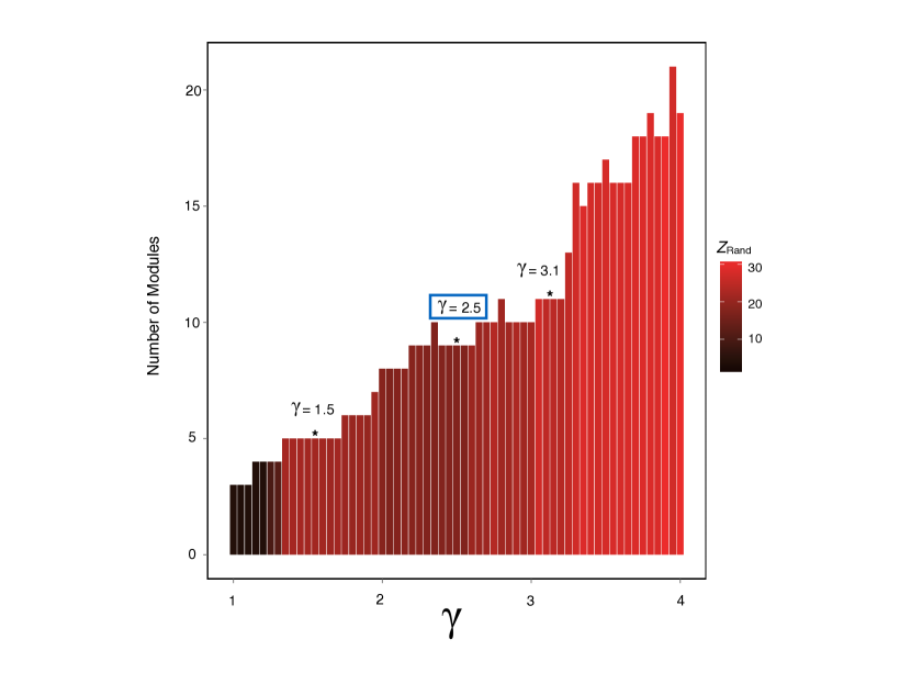
Supplemental Figure 1: Number of modules identified in group-level structural partitions. To examine alternative data-driven modular partitions of structural brain networks, we varied $\gamma$ over the interval $\left[0,4\right]$ in increments of 0.05. The number of modules identified in group-level consensus partitions increases as a function of $\gamma$. The similarity between structural partitions and a priori functional partitions also increases with $\gamma$ and the number of identified structural modules. $\ast$ indicates alternative structural partitions identified at plateaus for the number of modules. Bars are colored by the z-score of the Rand coefficient, which quantifies the similarity between structural partitions and the a priori functional partition used throughout the main text. The 9-module structural partition identified at $\gamma$=2.5 (marked by blue box) is used to examine age-related effects on modular segregation in Figure 5. The z-score of the Rand coefficient is equal to 17.6 (p $<$ $1\times 10^{-10}$) for this structural partition, suggesting a significant similarity with the functional partition beyond chance.

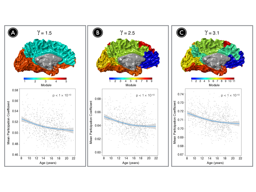
Supplemental Figure 2: Data-driven structural network modules become more segregated across youth. Here we demonstrate that regardless of the group-level consensus partition used to define modules, modular segregation increases with age, as demonstrated by a significant decrease in the mean participation coefficient. This developmental pattern is replicated using a 5-module partition (A, $\gamma$=1.5), a 9-module partition (B, $\gamma$=2.5), and an 11-module partition (C, $\gamma$=3.1). The 9-module partition pictured in B is used to calculate modular segregation in Figure 5. Blue line represents the best fit from a general additive model; shaded area indicates 95$\%$ confidence interval. Models include participant sex, in-scanner head motion, and total network strength as covariates.

Supplemental Experimental Procedures

Subjects

Diffusion tensor imaging (DTI) datasets were acquired as part of the Philadelphia Neurodevelopmental Cohort (PNC), a large community-based study of brain development. 1601 subjects completed the cross-sectional neuroimaging protocol (Satterthwaite et al., 2014). Datasets from 244 individuals were considered unusable due to incomplete acquisition or incidental findings. The remaining 1357 participants underwent a rigorous manual and automated quality assurance protocol for DTI datasets (Roalf et al., 2016), which flagged 157 subjects for poor data quality (e.g., low temporal signal-to-noise ratio). Of the remaining 1210 participants, 93 were flagged by automated quality assurance for low quality or incomplete FreeSurfer reconstruction of T1-weighted images. Of the remaining 1117 participants, 235 subjects were excluded for meeting any of the following criteria: gross radiological abnormalities, history of medical problems that might affect brain function, history of inpatient psychiatric hospitalization, use of psychotropic medication at the time of data acquisition, missing data, and/or high levels of in-scanner head motion (mean relative displacement between non-weighted volumes $>$ 2mm), which has been shown to impact measures derived from diffusion-weighted imaging (Roalf et al., 2016; Yendiki et al., 2013). These exclusions produced a final sample consisting of 882 youths (mean age=15.06, SD=3.15; 389 males, 493 females).

Cognitive Assessment

The Penn computerized neurocognitive battery (Penn CNB) was administered to all participants. The CNB consists of 14 tests adapted from tasks applied in functional neuroimaging to evaluate a broad range of cognitive domains (Gur et al., 2002; Gur et al., 2012). These domains include executive control (abstraction and flexibility, attention, working memory), episodic memory (verbal, facial, spatial), complex cognition (verbal reasoning, nonverbal reasoning, spatial processing), social cognition (emotion identification, emotion intensity differentiation, age differentiation) and sensorimotor and motor speed. Accuracy and speed for each test were z-transformed. Cognitive performance was summarized by a recent factor analysis (Moore et al., 2014) of both speed and accuracy data, which delineated three factors corresponding to the efficiency of executive function, episodic memory, and social cognition.

Data Acquisition

All MRI scans were acquired on the same 3T Siemens Tim Trio whole-body scanner and 32-channel head coil at the Hospital of the University of Pennsylvania. DTI scans were acquired using a twice- refocused spin-echo (TRSE) single-shot echo-planar imaging (EPI) sequence (TR = 8100ms, TE = 82ms, FOV = 240mm2 /240mm² ; Matrix = RL: 128/AP:128/Slices:70, in-plane resolution (x and y) 1.875 mm²; slice thickness = 2mm, gap = 0; flip angle = 90^∘/180^∘/180^∘, volumes = 71, GRAPPA factor = 3, bandwidth = 2170 Hz/pixel, PE direction = AP). This sequence used a four-lobed diffusion encoding gradient scheme combined with a 90-180-180 spin-echo sequence designed to minimize eddy-current artifacts . DTI data were acquired in two consecutive series consisting of 32 diffusion encoding gradient schemes. The complete sequence consisted of 64 diffusion-weighted directions with b=1000s/mm² and 7 interspersed scans where b=0 s/mm². The duration of DTI scans was approximately 11 minutes. The imaging volume was prescribed in axial orientation covering the entire cerebrum with the topmost slice just superior to the apex of the brain (Satterthwaite et al. 2014a). In addition to the DTI scan, a map of the main magnetic field (i.e., B0) was derived from a double-echo, gradient-recalled echo (GRE) sequence, allowing us to estimate field distortions in each dataset.

Data Preprocessing

Two consecutive 32-direction acquisitions were merged into a single 64-direction time-series. The skull was removed for each subject by registering a binary mask of a standard fractional anisotropy (FA) map (FMRIB58 FA) to each subject’s DTI image using a rigid-body transformation (Smith et al., 2002). Eddy currents and subject motion were estimated and corrected using FSL’s eddy tool (Andersson and Sotiropoulos 2016). Diffusion gradient vectors were then rotated to adjust for subject motion estimated by eddy. After the field map was estimated, distortion correction was applied to DTI data using FSL’s FUGUE (Jenkinson et al., 2012). Lastly, DTI data was imported into DSI Studio software and the diffusion tensor was estimated at each voxel.

DTI Tractography

Whole-brain fiber tracking was implemented for each subject in DSI Studio using a modified fiber assessment by continuous tracking (FACT) algorithm with Euler interpolation, initiating 1,000,000 streamlines after removing all streamlines with length less than 10mm or greater than 400mm (Yeh et al., 2013). Fiber tracking was performed with an angular threshold of 45^∘, a step size of 0.9375mm, and a fractional anisotropy (FA) threshold determined empirically by Otzu’s method, which optimizes the contrast between foreground and background (Yeh et. al., 2013). Diffusivity measures (e.g., FA, mean diffusivity, radial diffusivity, axial diffusivity) were calculated along the path of each reconstructed streamline. For each subject, tractography served as the basis for constructing structural brain networks.

Network Construction

Following T1 reconstruction in FreeSurfer (version 5.3), cortical and subcortical gray matter was parcellated according to the Lausanne atlas (Cammoun et al., 2012), which includes whole-brain parcellations at multiple spatial scales (83, 129, 234, 463, and 1015 regions). Parcellations were defined in native space and co-registered to the first $b=0$ volume of each subject’s diffusion image using a rigid-body transform. To extend gray matter region labels beyond the gray-white boundary, the atlas labels were dilated by 4mm (Gu et al., 2015). Dilation involved filling non-labelled voxels with the statistical mode of neighboring labels. 234 dilated brain regions defined the nodes for each subject’s structural brain network, which was represented as a weighted adjacency matrix $A$. Edges were defined where at least one streamline connected a pair of nodes end-to-end. Edge weights were primarily defined by the average FA along streamlines connecting any pair of nodes (Misic et al., 2016; Bohlken et al., 2016). See Figure 2.

Functional Module Assignment

For the 234- and 463-region parcellations, we calculated a purity index for each Lausanne label and corresponding voxels in the standard 7-system template image provided by Yeo et al. (2011). This measure quantifies the maximum overlap of cortical Lausanne labels and functional systems defined by Yeo et al. (2011). Each cortical Lausanne label was assigned to a functional system by calculating the non-zero mode of all voxels in each brain region. Subcortical regions were assigned to an eighth, subcortical module. The primary modular partition defined for 234-node networks is shown in Figure 2. To determine whether the functionally-defined network partition significantly fit the structural connectivity data beyond chance, we quantified the modularity quality index (formally defined below) of the functional partition imposed on structural brain networks. Briefly, the modularity quality of a network partition quantifies how well that partition maximizes the strength of within-module connections relative to a specified null model. Higher $Q$ values indicate that modules are highly segregated within a network, with strong within-module connectivity and relatively weak between-module connectivity. We performed a permutation test to examine the significance of the modularity quality of the functional partition ($Q_{Yeo}$) imposed on structural connectivity matrices. First, we permuted the assignment of $N$ nodes to functional modules 1000 times, preserving the number of nodes originally assigned to each module. We then calculated the modularity quality $Q_{perm}$ of randomly-defined network partitions imposed on each subject’s connectivity matrix, building a null distribution for $Q_{perm}$. We used the calculated mean ($\mu_{Q_{perm}}$) and standard deviation ($\sigma_{Q_{perm}}$) of the null distribution to derive a z-score based on the observed $Q_{Yeo}$ for each subject (z-score = $\frac{(Q_{Yeo}-\mu_{Q_{perm}})}{\sigma_{Q_{perm}}}$). Finally, we calculated the mean z-score across all subjects to assess the significance of $Q_{Yeo}$.

Measures of Modular Segregation

We calculated the participation coefficient to quantify the relative balance of between-module versus within-module connectivity for each brain region. Intuitively, this measure describes the degree to which a brain region integrates information across distinct modules, or the degree to which a brain region shows provincial connectivity among regions in its own module. We define the participation coefficient $P_{i}$ of node $i$ as

$$P_{i}=1-\sum_{m\in{M}}\Big{(}\frac{k_{i}(m)}{k_{i}}\Big{)}^{2},$$ (1)

where $m$ is a module in a set of modules $M$, and $k_{i}(m)$ is the weight of structural connections between node $i$ and all nodes in module $m$ (Guimera and Amaral 2005; Rubinov and Sporns 2010). Moreover, $P_{i}$ close to 1 indicates that a brain region is highly integrated with regions in other modules, while a $P_{i}$ close to 0 indicates that a brain region is highly segregated, with strong connectivity among other regions in its own module. To quantify the segregation of specific modules, we average $P_{i}$ across all brain regions assigned to the same module. To quantify global network segregation, we average $P_{i}$ across all nodes in the network.

Alternative Measures of Modular Segregation

To ensure that our results were not dependent on specific network metrics, we calculated alternative measures of modular segregation. First, we calculated the average strength of all within-module connections (a measure of structural coherence), and the average strength of all between-module connections (a measure of structural integration) in the network (Gu et al., 2015). These metrics provide additional insights into the segregation of information processing within distinct modules, and the degree to which modules are integrated across the network (see Figure 4). Alternatively, we calculated the subject-specific modularity quality ($Q$) of group-level functional and structural network partitions. As discussed above, this measure provides an index of how well a network can be decomposed into a hard partition where nodes within the same module demonstrate particularly strong connectivity beyond chance. We also calculated $Q_{subj}$ for subject-specific consensus partitions (see detailed procedure below), which was not dependent on a group-level partition. We calculated the modularity $Q$ of a network partition $S$ based on the following modularity quality function:

$$Q(S)=\frac{1}{2m}\sum_{ij}\Big{[}A_{ij}-\gamma P_{ij}\Big{]}\delta(g_{i},g_{j}),$$ (2)

where $m$ is the total weight of $A$, $P$ represents the expected strength of connections according to a specified null model (Newman, 2004), $\gamma$ is a structural resolution parameter that determines the size of modules, and $\delta(g_{i},g_{j})$ is equal to unity when brain regions $i$ and $j$ are assigned to same community $g_{i}$, and is zero otherwise.

Community Detection in Structural Brain Networks

Primary analyses relied on an a priori functional partition to define network modules. We additionally estimated network modules directly from the structural connectivity data using community detection procedures. Communities were defined by maximizing the modularity quality function using a generalization of the Louvain heuristic (Blondel et al., 2008; Mucha et al., 2010). Because the Louvain algorithm is degenerate (Good et al., 2010; Sporns and Betzel 2016), it is essential to perform modularity maximization multiple times in order to identify a stable consensus partition that accurately reflects the solutions offered by each optimization. Accordingly, we applied a locally greedy Louvain-like modularity-optimization procedure (Blondel et al., 2008) 100 times for each subject in order to define an “agreement” matrix $\mathbf{\mathit{A^{\prime}}}$ where $A_{ij}^{\prime}$ was equal to the probability that nodes $i$ and $j$ were assigned to the same community over the 100 iterations. If $\mathbf{\mathit{A^{\prime}}}$ was deterministic (edge weights were binary), then the algorithm had converged and the resultant partition was defined as the consensus. Otherwise, we performed 100 iterations of modularity optimization on $\mathbf{\mathit{A^{\prime}}}$ in order to generate a new agreement matrix $\mathbf{\mathit{A^{\prime\prime}}}$. This procedure was repeated until convergence (Lancichinetti and Fortunato, 2014). When performing modularity optimization on an agreement matrix (e.g., $A^{\prime}$ or $A^{\prime\prime}$), we defined an alternative null model $P^{\prime}$ by permuting community assignments across nodes (Bassett et al., 2013).

Once a consensus partition was identified for each subject, we computed a group-level consensus across the full PNC cohort (n=882). To do this, we used a Louvain-like procedure to detect communities in a group-level agreement matrix $A_{group}^{\prime}$. Edge weights in $\mathbf{\mathit{A_{group}^{\prime}}}$ were equal to the proportion of times that each pair of nodes was assigned to the same community across subject-level consensus partitions. As above, 100 iterations of modularity optimization were performed on $\mathbf{\mathit{A_{group}^{\prime}}}$ until the resulting $\mathbf{\mathit{A_{group}^{\prime\prime}}}$ became binary, indicating that the algorithm had converged on a group-level consensus partition. Both subject-level and group-level consensus partitions were computed over a wide range of $\gamma$ ($\left[0,4\right]$, in increments of 0.05) to explore variations in community structure. We plotted the number of group-level consensus modules as a function of $\gamma$, and found several plateaus indicating partition stability (Fenn et al., 2009; see Figure S1). In order to directly compare the organization of data-driven, modularity-based partitions and the a priori functional partition, we quantified the partition similarity using the $z$-score of the Rand coefficient (Traud et al., 2011). For two partitions $X$ and $Y$, we calculated the Rand $z$-score in terms of the total number of node pairs in the network $M$, the number of pairs $M_{X}$ assigned to the same module in partition $X$, the number of pairs $M_{Y}$ that are in the same module in partition $Y$, and the number of pairs of nodes $w_{XY}$ that are assigned to the same module both in partition $X$ and in partition $Y$. The $z$-score of the Rand coefficient is defined by:

$$z_{XY}=\frac{1}{\sigma_{w_{XY}}}w_{XY}-\frac{M_{X}M_{Y}}{M},$$ (3)

where $\sigma_{w_{XY}}$ is the standard deviation of $w_{XY}$. The mean partition similarity is determined by the mean value of $z_{XY}$ over all possible partition pairs for $X\neq Y$. Moreover, $z_{XY}$ denotes the similarity of partitions $X$ and $Y$ beyond chance. Figure S1 shows the similarity between all group-level structural partitions and the primary functional partition used in this study.

Measures of Network Integration

For each subject’s structural brain network $A$, the topological length or distance of each edge $A_{ij}$ was computed as the reciprocal of the edge weight ($\frac{1}{A_{ij}}$). The path length between any pair of nodes is defined as the sum of the edge lengths along the shortest path connecting them (Rubinov and Sporns, 2010). Global efficiency provides a theoretical prediction of how easily information can flow across a network via the shortest path between all pairs of nodes, and is defined by

$$E_{glob}(G)=\frac{1}{n}\sum_{i\in{N}}\frac{\sum_{j\in{N},j\neq{i}}\bigg{(}d_{ij}\bigg{)}^{-1}}{n-1},$$ (4)

where $n$ is the number of nodes, and $d_{ij}$ is the shortest path length between node $i$ and node $j$.

To examine the possible role of specific edges as integrative hub connections within the network, we calculated the weighted edge betweenness centrality ($EBC$) for each edge. Edge betweenness identifies important hub connections by providing a measure of how much a given connection participates in the shortest paths of communication through a network, and thus contributes to global efficiency (Brandes, 2001).

$$EBC=\sum_{hk}\frac{\rho_{hk}^{ij}}{\rho_{hk}},$$ (5)

where $\rho_{hk}^{ij}$ denotes the number of shortest paths between nodes $h$ and $k$ that include edge $ij$, and $\rho_{hk}$ denotes the total number of shortest paths between $h$ and $k$. After calculating $EBC$ individually for each weighted network $A_{ij}$ (n=882), we normalized each subjects^′ $EBC$ values by their maximum observed $EBC$, resulting in a bounded measure $\left[0,1\right]$ (Gong et al., 2009). We calculated the mean normalized $EBC$ for each network edge across subjects, and defined hub edges as those connections within the top quartile of normalized edge betweenness across all network edges. Following group-level analysis, which identified a subset of edges that significantly strengthened with age, we performed a permutation-based test to assess whether connections that significantly strengthened with age were enriched for hub edges (see below).

Group-level analyses

Prior work has demonstrated that brain development is not a linear process (Paus et al., 1999, Shaw et al., 2006). Accordingly, group-level analyses of structural brain network metrics were flexibly modeled using penalized splines within a General Additive Model (GAM) implemented in the R package “mgcv” (https://cran.r-project.org/web/packages/mgcv/index.html; Wood 2004; Wood 2011). Such an approach allows for detection of nonlinearities in the relationship between age and measures of modular segregation without defining a set of functions a priori (such as polynomials). Importantly, the GAM estimates nonlinearities using restricted maximum likelihood (REML), and determines a penalty with increasing nonlinearity in order to avoid overfitting the data. Due to this penalty, the GAM only models nonlinearities when they explain additional variance in the data above and beyond linear effects.

First, we used penalized splines to estimate nonlinear developmental patterns of modular segregation. Within this model we included covariates for sex, head motion, and total network strength. Accordingly, the final model equations for estimating age effects on modular segregation (mean participation coefficient) were as follows:

Modular segregation = spline(age) + sex + motion + total network strength

An identical model was used when estimating age effects on the participation coefficient of individual brain regions. Similarly, we applied this model across all network edges in order to assess linear and nonlinear age effects on the strength of individual connections. For all analyses, multiple comparisons were controlled using the False Discovery Rate (q$<$0.05).

Permutation Testing

We performed permutation-based tests across network edges in order to assess (i) whether the edges that significantly strengthened with age were localized to within-module connections beyond chance, (ii) whether edges that significantly strengthen with age were enriched for hub edges, and (iii) whether these ages had elevated edge betweenness centrality beyond chance.

First, we permuted a binary edge label specifying whether each edge connects nodes within or between modules 1000 times. Then for permuted samples of within- and between-module edges, we counted the number of edges that were shown to significantly strengthen with age in group-level analysis. We then rank-ordered the number of edges shown to significantly strengthen with age for permuted within-module edge samples, and determined where the observed number of within-module edges that strengthen with age falls relative to this null distribution.

Second, we evaluated whether edges that significantly strengthen with age were enriched for hub edges. We permuted a binary edge label defining hub or non-hub edges 1000 times. For each permuted sample, we counted the number of edges that significantly strengthened with age in group-level analysis. Then, we rank-ordered the number of permuted hub edges shown to significantly strengthen with age, and compared these values with the observed number of hub edges that strengthened with age.

Third, we evaluated whether edges that significantly strengthen with age had higher edge betweenness centrality than anticipated by chance. We permuted normalized edge betweenness centrality values 1000 times. For each permuted sample, we calculated the mean $EBC$ of within-module edges and between-module edges that significantly strengthened with age. We rank-ordered the mean $EBC$ of permuted within-module and between-module edges that strengthened with age, and compared these values with the observed means for within- and between-module edges separately (Figure 6D).

Methodological Replications

To verify that observed age-related increases in modular segregation were not simply due to specific network construction choices, we repeated developmental inferences on modular segregation using a variety of other parameters. First, we examined age effects on modular segregation (mean participation coefficient) using a data-driven structural partition identified at the group level (see Figure S2B., Figure 5B, and detailed procedure above). Alternatively, we also calculated the modularity quality index for each subject^′s optimal partition at $\gamma$=2.5 ($Q_{Subj}$), where a higher $Q_{Subj}$ indicates greater modular segegration (Figure 5C). Next, we examined modular segregation (mean participation coefficient) using the a priori functional partition assigned to a higher-resolution parcellation of the brain (463 nodes instead of 234; see Figure 5D). We also measured modular segregation of the functional partition using structural networks with alternative edge weight definitions. While primary analyses focused on FA-weighted structural networks, we also measured modular segregation in streamline-weighted networks (see Figure 5E), where edge weights were equal to the number of streamlines connecting a pair of nodes (Bassett et al., 2011), and additionally, where edge weights were defined by streamline density: the number of connecting streamlines divided by the total regional volume of each node pair (Baker et al., 2015; see Figure 5F). In addition to examining age-related patterns of modular segregation using alternative network measures and parameters, we also repeated analyses including the following additional covariates in the GAM described above: race, maternal education, handedness, and total brain volume.

Relationship Between Modular Segregation and Global Network Efficiency

First, we examined age-related effects on global efficiency using the same GAM as above:

Global efficiency = spline(age) + sex + motion + total network strength

(see Figure 6A). The relationship between global efficiency and modular segregation was assessed within a GAM while controlling for age in addition to other covariates described above (Figure 6B). Moreover, the model equation was as follows:

Modular segregation = Global efficiency + spline(age) + sex + motion + total network strength

To assess whether global efficiency was related to the weight of specific network connections that strengthened with age, we estimated the following GAMs:

Global efficiency = Average strength of within-module edges + spline(age) + sex + motion + total network strength

Global efficiency = Average strength of between-module edges + spline(age) + sex + motion + total network strength

(see Figure 6E and Figure 6F).

Associations with Executive Function

To examine the association between modular segregation and executive efficiency, we included a spline age term in the model to account for the variance associated with linear and nonlinear age-related changes in executive ability. The final model equation was as follows:

Modular segregation = spline(age) + executive efficiency + sex + motion + total network strength

Using the same GAM, we also evaluated the association between the segregation of individual modules (e.g., frontoparietal) and three cognitive efficiency factor scores: executive function, memory, and social cognition (see Figure 7A). We note that 2 participants of the full 882 sample had incomplete cognitive datasets: subsequent analyses examining associations between executive function and modular segregation focused on the remaining 880 participants. Visualization of GAM model fits were created using the “visreg” package in R (https://cran.r-project.org/web/packages/visreg/). In Figure 3A, Figure 5, and Figure 6B, one outlying datapoint was beyond the axis range, and was excluded for visualization purposes only: group-level analyses and reported results include data points for all subjects.

Mediation analyses

Linear mediation analyses investigated whether age-related improvement in executive function was mediated by modular segregation and/or global efficiency (Preacher and Hayes, 2008). First, we regressed out the effects of nuisance covariates (sex, head motion, and total network strength) on the independent (X), dependent (Y), and mediating (M) variables. The residuals were then used in our mediation analysis. The significance of the indirect effect was evaluated using bootstrapped confidence intervals within the R package “lavaan” (https://cran.r-project.org/web/packages/lavaan/). Specifically, we examined the total effect of age on executive performance (c path; Figure 7B), the relationship between age and modular segregation (a path), the relationship between modular segregation and executive function (b path), and the direct effect of age on executive efficiency after including modular segregation as a mediator in the model (c^′ path). The significance of the indirect effect of age on executive function through the proposed mediator (modular segregation) was tested using bootstrapping procedures, which minimize assumptions about the sampling distribution (Preacher and Hayes, 2008). This approach involves calculating unstandardized indirect effects for each of 10,000 bootstrapped samples and calculating the 95$\%$ confidence interval. This procedure was repeated to assess (i) whether the segregation of the frontoparietal module mediated developmental improvements in executive function, (ii) whether the segregation of the default mode module mediated developmental improvements in social cognition, and (iii) whether age-related increases in global efficiency mediated improvements in executive function.

Data Visualization

Network partitions and regional results (Figure 2, Figure 3C, and Figure S2) were visualized on the cortical white matter surface using FreeSurfer visualization tools in MATLAB. While age effects on the participation coefficient for subcortical brain regions are not visualized in Figure 3C, these regions were included in all analyses. Brain network visualizations in Figure 4 and Figure 6 were generated using BrainNet Viewer (Xia et al. 2013).

Supplemental References

1. Andersson, J.L. and Sotiropoulos, S.N. (2016). An integrated approach to correction for off-resonance effects and subject movement in diffusion MR imaging. Neuroimage, 125,1063-1078.

2. Bassett, D.S., Porter, M.A., Wymbs, N.F., Grafton, S.T., Carlson, J.M. and Mucha, P.J. (2013). Robust detection of dynamic community structure in networks. Chaos, 23, 013142.

3. Fenn, D.J. Porter, M.A., McDonald, M., Williams, S., Johnson, N.F., and Jones, N.S. (2009). Dynamic communities in multichannel data: An application to the foreign exchange market during the 2007-2008 credit crisis. Chaos 19, 033119.

4. Giedd, J.N., Blumenthal, J., Jeffries, N.O., Castellanos, F.X., Liu, H., Zijdenbos, A., Paus, T., Evans, A.C., Rapoport, J.L. (1999). Brain development during childhood and adolescence: a longitudinal MRI study. Nature Neuroscience 2(10), 861-3.

5. Gong, G., He, Y., Concha, L., Lebel, C., Gross, D.W., Evans, A.C. and Beaulieu, C. (2009). Mapping anatomical connectivity patterns of human cerebral cortex using in vivo diffusion tensor imaging tractography. Cerebral Cortex, 19, 524-536.

6. Good, B. H., Montjoye, Y., and Clauset, A. (2010). Performance of modularity maximization in practical contexts. Physical Review E 81, 046106.

7. Gu, S., Pasqualetti, F., Cieslak, M., Telesford, Q.K., Alfred, B.Y., Kahn, A.E., Medaglia, J.D., Vettel, J.M., Miller, M.B., Grafton, S.T. and Bassett, D.S. (2015). Controllability of structural brain networks. Nature Communications, 6.

8. Lancichinetti, A. and Fortunato, S., 2012. Consensus clustering in complex networks. Scientific reports, 2.

9. Newman, M.E.J., 2004. Analysis of weighted networks. Physical Review E, 70, 056131.

10. Paus, T., Zijdenbos, A., Worsley, K., Collins, D.L., Blumenthal, J., Giedd, J.N., Rapoport, J.L. and Evans, A.C. (1999). Structural maturation of neural pathways in children and adolescents: in vivo study. Science, 283, 1908-1911.

11. Shaw, P., Greenstein, D., Lerch, J., Clasen, L., Lenroot, R., Gogtay, N.E.E.A., Evans, A., Rapoport, J. and Giedd, J. (2006). Intellectual ability and cortical development in children and adolescents. Nature, 440, 676-679.

12. Xia, M., Wang, J. and He, Y. (2013). BrainNet Viewer: a network visualization tool for human brain connectomics. PLoS One, 8, e68910.