On the forced flow around a flapping foil.

Abstract

The two dimensional incompressible viscous flow past a flapping foil immersed in a uniform stream is studied numerically. Numerical simulations were performed using a Lattice-Boltzmann model for moderate Reynolds numbers. The computation of the hydrodynamic force on the foil is related to the the wake structure. In particular, when the foil’s centre of mass is fixed in space, numerical results suggest a relation between drag coefficient behaviour and the flapping frequency which determines the transition from the von Kármán (vKm) to the inverted von Kármán wake. Beyond the inverted vKm transition the foil was released. Upstream swimming was observed at high enough flapping frequencies. Computed hydrodynamic forces suggest the propulsion mechanism for the swimming foil.

1 Introduction

The flow around a flapping foil has been studied in a variety of conditions. Foils on a stream, flapping as a result of the hydrodynamic forces acting on them, have been studied in connection to energy extraction processes  (Wu et al., 2015; Wu, 1972). The wake of foils with an imposed flapping and translational motion, and its relation with the reacting forces on them has deserved attention due to its relation to flying and swimming (Anderson et al., 1998; Dong et al., 2006; Triantafyllou et al., 2000; Taylor et al., 2003). Little has been done in the case of an imposed flapping on a foil free to swim, although work can be found related to other type of swimmers at moderate Reynolds numbers (Kern and Koumoutsakos, 2006; Gemmell et al., 2015; Chisholm et al., 2016). Here we study numerically a two-dimensional foil with an imposed flapping motion, immersed in a stream, that can be released and become free of translational motion. Both phenomena were studied and compared for moderate Reynolds numbers, where inertia and viscous forces are important.

We used the lattice Boltzmann model (LBM) of He et al. (1998), with a procedure to include immersed moving boundaries of arbitrary shape subject to hydrodynamic forces (Mandujano and Rechtman, 2008). The LBM is an efficient algorithm to approximate solutions to the Navier- Stokes equations when implemented on massively parallel architectures, where it can handle simulations of high resolution and large computational domains (Clausen et al., 2010). For the problem in hand the LBM seemed a good option, since wakes behind objects may show interesting behaviour far away behind the object (Vorovieff et al., 2002), and so a large domain relative to the size of the foil was desirable, along with enough resolution to observe vortex formation and evolution.

The article is divided as follows, in section 2 the general problem is presented and the numerical method used is described briefly in section 3. In section 4 the results are presented and discussed. Conclusions are summarised in in section 5.

2 Statement of the problem

Consider an unbounded two dimensional and incompressible flow of a viscous fluid around a rigid flapping foil made by a semicircle, with diameter $D$, intersected with an isosceles triangle of high $h$, as shown in figure 1.

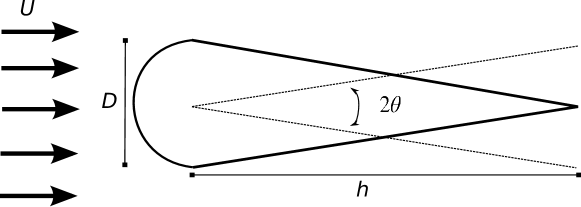
Figure 1: Schematic illustration of the flow around a flapping foil.

Two cases are considered, a foil with a point fixed in space and a foil free to move. In both cases the flapping motion consist of an oscillation with respect to the centre of the semicircle, which is fixed in space in one case and free in the other. To simplify the calculations, it is assumed that the foil mass density distribution, $\rho_{s}$, is such that its centre of mass is at the centre of the semicircle.

The governing equations for the fluid, with mass density $\rho_{f}$ and kinematic viscosity $\nu$, are the Navier-Stokes equations given by

$$\nabla\cdot\boldsymbol{u} = 0,$$ (1)

$$\frac{\partial\boldsymbol{u}}{\partial t}+\boldsymbol{u}\cdot\nabla\boldsymbol{u} = -\frac{1}{\rho_{f}}\nabla P+\nu\nabla^{2}\boldsymbol{u},$$ (2)

where $\boldsymbol{u}(\boldsymbol{r},t)$ and $P(\boldsymbol{r},t)$ are the velocity and pressure fields, respectively. Consider no-slip condition at the foil’s surface. Constant pressure and a uniform and horizontal velocity field $\boldsymbol{U}$ are imposed far from the foil (see figure 1).

The rigid foil is forced to rotate around the centre of the semicircle (also its centre of mass) so that the angle of its axis of symmetry with respect to the horizontal coordinate evolve with $\theta(t)=\theta_{0}\sin\omega t$ (see Figure 1). The velocity of a point at the foil’s surface is $\boldsymbol{v}_{s}({\bf r}_{s},t)=\boldsymbol{V}(t)+\dot{\theta}(t)(\boldsymbol{r}_{s}-\boldsymbol{R})$, where $\boldsymbol{R}$ is the position of the centre of mass, $\boldsymbol{V}$ its velocity and $\boldsymbol{r}_{s}$ is the position of a point at the foil’s surface. Therefore, the no-slip boundary condition takes the form $\boldsymbol{u}(\boldsymbol{r}_{s},t)=\boldsymbol{v}_{s}(\boldsymbol{r}_{s},t)$. In the case of the free flapping foil, the motion of its centre of mass is obtained by solving $md\boldsymbol{V}/dt=\boldsymbol{F}$, where $m$ is the mass of the foil. The hydrodynamical force $\boldsymbol{F}$ acting on the foil, is obtained directly from the computed flow fields.

To work with non-dimensional variables we choose $D$ as the characteristic length, $U$ as the characteristic velocity and the fluid density $\rho_{f}$. With this choice of scaling the flow regime is determined by five dimensionless parameters: the Reynolds number $\mbox{{Re}}=UD/\nu$, the Strouhal number $St=\omega D/2\pi U$ the dimensionless amplitude $A=2\theta_{0}h/D$, the ratio between the chord of the foil and the circle’s diameter $C=1/2+h/D$, and the fluid-foil’s mass density ratio $\mu=\rho_{f}/\rho_{s}$ which is set to unity to work with a non-buoyant foil. The hydrodynamic force is scaled with $\rho_{f}U^{2}D/2$. We define the drag $C_{D}$ and lift $C_{L}$ coefficients as the horizontal and vertical components of $2\boldsymbol{F}/\rho_{f}U^{2}D$, respectively. Notice that negative values of $C_{D}$ correspond to a thrust dominated hydrodynamic force.

Solutions to equations (2) and (1) for the pressure and velocity fields are approximated using a lattice-Boltzmann model. The numerical procedures are described in the following section.

3 The numerical scheme

To compute the flow around the flapping foil a two dimensional, nine neighbours (D2Q9) lattice-Boltzmann model was used (He et al., 1998). The proposed algorithm, that includes moving immersed boundaries, was validated in a previous work concerning a problem of a moving cylinder in a convective flow (Mandujano and Rechtman, 2008).

In this method space is discretised using a square lattice. Lattice spacing as well as time steps can be conveniently set to unity. The state of the fluid at the node with vector position $\boldsymbol{r}$ at time $t$, is described by the particle distribution function $f_{k}(\boldsymbol{r},t)$ that evolves in time and space according to

$$f_{k}(\boldsymbol{r}+\boldsymbol{e}_{k},t+1)=f_{k}(\boldsymbol{r},t)-\dfrac{1}{\tau}\left[f_{k}(\boldsymbol{r},t)-f_{k}^{(eq)}(\boldsymbol{r},t)\right],$$ (3)

where $\tau$ is a relaxation time related to the fluid kinematic viscosity $\nu=(\tau-1/2)/3$. The distribution function $f_{k}^{(eq)}$ is given by

$$f_{k}^{(eq)}(\boldsymbol{r},t)=w_{k}\rho\left(1+3\boldsymbol{e}_{k}\cdot\boldsymbol{u}+\dfrac{9}{2}(\boldsymbol{e}_{k}\cdot\boldsymbol{u})^{2}-\frac{3}{2}\boldsymbol{u}^{2}\right),$$ (4)

which corresponds to a discrete Maxwell distribution function for thermal equilibrium. In the above expressions, the macroscopic density and velocity fields are computed using

$$\rho(\boldsymbol{r},t)=\sum_{k}f_{k}(\boldsymbol{r},t)\quad\textmd{and}\quad\rho{\boldsymbol{u}}(\boldsymbol{r},t)=\sum_{k}\boldsymbol{e}_{k}f_{k}(\boldsymbol{r},t).$$

The microscopic set of velocities $\boldsymbol{e}_{k}$ is given by

$$\boldsymbol{e}_{0}=(0,0),\quad\boldsymbol{e}_{k}=\left(\cos(\pi(k-1)/2),\sin(\pi(k-1)/2)\right)\ \ \textmd{for}\ \ k=1,\dots,4,$$

$$\boldsymbol{e}_{k}=\sqrt{2}\left(\cos(\pi(k-9/2)/2),\sin(\pi(k-9/2)/2)\right)\ \ \textmd{for}\ \ k=5,\dots,8,$$

where $w_{0}=4/9$, $w_{k}=1/9$ for $k=1,\dots,4$ and $w_{k}=1/36$ for $k=5,\dots,8$. Notice that, with the choice of microscopic velocities $\boldsymbol{e}_{k}$, expression (3) is always evaluated at lattice points. It is well known that the above procedure approximates solutions to the Navier-Stokes equations in the limit of small Mach numbers (He et al., 1998).

Equation (3) provide an explicit algorithm for updating all the distribution functions $f_{k}$ at a given node in the lattice, as long as its 8 nearest neighbouring nodes are inside the fluid domain. For nodes adjacent to a solid wall, the distribution functions coming from neighbouring nodes outside the fluid domain must be provided as a boundary condition for the method. We choose to adopt the set of boundary conditions proposed by Guo and Zheng (2002) for curved rigid walls.

The force and torque acting on the body are computed using the momentum-exchange method of Mei et al. (2002). For the free flapping foil, as rotational motion is imposed, only the force is used to compute the foils translational motion using a forward Euler integration in time at each time step. This is a particular case of the scheme described in Mandujano and Rechtman (2008) for the motion of a free particle in a convective flow using the lattice-Boltzmann model.

The computational domain was a rectangular lattice of $10000\times 3000$ nodes for the fixed foil, and of $12000\times 5000$ nodes for the free foil. The foil had a length $h$ of 280 to 600 nodes, a width $D$ of 80 nodes (about a $1/30$ of the width and length of the domain), and was placed at 3000 nodes from the left boundary of the domain ($5$ foil lengths). To simulate conditions far from the foil, the velocity was set to $\boldsymbol{U}$ at the left boundary following the procedure of Guo and Zheng (2002). On the rest of the boundaries, the normal components of the velocity gradients were set to zero setting the unknown velocity at the boundary equal to that of the adjacent node normal to the wall.

The numerical scheme was implemented to run in parallel in GPU’s due to the large number of nodes involved in the simulations. Typically, two days are needed to obtain a periodic flow ($3\times 10^{5}$ time steps) of a free foil swimming upstream running on an Nvidia®Tesla K40 processor.

4 Results

The foil profile geometry was chosen to compare with experiments performed by Schnipper et al. (2009) in a soap films and by Godoy-Diana et al. (2008) in a wind tunnel. Numerical results confirm the relation between the drag-trust transition and the behaviour of the von Karman (vKm) vortex street.

4.1 A fixed flapping foil

Simulations start with the foil at rest facing a uniform flow at the left boundary to allow for a wake to form before flapping. After $5\times 10^{4}$ time steps, the foil starts to flap increasing its amplitude exponentially in time until it reaches $A$. The simulations were performed for a series of values of $St\in[0.1,0.6]$, $A\in[0.5,3]$, $Re\in[100,255]$, and $C$ took values $4$ and $6$.

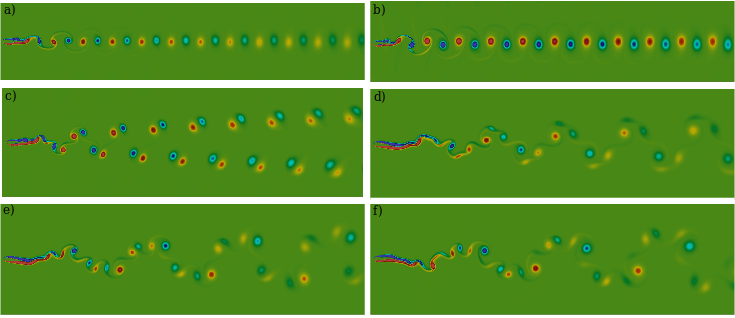
Figure 2: Vorticity distribution for a fixed flapping foil for $\mbox{{Re}}=220$. Colours represent positive (red) and negative (blue) vorticity. a) vKm wake for $St=0.12$ and $A=0.98$. b) inverted vKm wake for $St=0.12$ and $A=2$. c) 2P wake for $St=0.085$ and $A=1.4$. d) 2P+2S wake for $St=0.05$ and $A=1.4$. e) 4P wake for $St=0.035$ and $A=1.34$. f) 4P+2S wake for $St=0.025$ and $A=1.2$. Figures show the region of interest within the computational domain.

Following Schnipper et al. (2009), in the first set of simulations $\mbox{{Re}}=220$ and $C=6$. The simulations performed show the formation of patterns in approximately the same parameter region as reported there (see Figure 2); transitions between vKm and inverted vKm wake, formation of 2P, 4P, 2P+2S, 4P+2S wakes (following the nomenclature of Williamson and Govardhan (2004)) and the transitions between them. Quantitative comparison can not be expected as film flow is not a two dimensional phenomena.

The computed hydrodynamical force on the foil showed a periodic dependence on time (see Figure 3). When the flow has 2S or 2P wakes (Figures 2-(a)-(c)), the lift coefficient $C_{L}$ oscillates with the flapping frequency, corresponding to a Fourier mode $n=1$. The drag coefficient $C_{D}$ oscillates with twice the flapping frequency and has modes $n=0$ and $n=2$. Notice that $C_{D}$ minima (maximum thrust) is obtained after extremal values of the angle of attack $\theta$ are reached.

The flapping frequency sets the hydrodynamic force frequencies and higher harmonics. For patterns with combinations of 2P, 4P and 2S, Fourier coefficients corresponding to higher harmonics become important. In Figure 2-(d)-(f), the lift and torque coefficients are composed by the first few odd modes while $C_{D}$ modes are even (see Figure 3-(a)). In the combination 2P+2S, $C_{D}$ have $n=2$ and 4 wile $C_{L}$ is composed by $n=1$ and $3$ modes. The 4P wake includes modes $n=6$ and $n=7$ and the 4P+2S wake has $n=8$ and $n=9$ modes. $C_{D}$ always showed even modes while $C_{L}$ modes were all odd. There is a strong horizontal push with every stroke and higher harmonics are produced at low flapping frequencies where many vortices are shed during each stroke.

When $St=0.12$ and $A\in[0.98,3]$ there is a transition between the vKm and the inverted vKm wake, known to be relate with the drag-thrust transition (Kármán and Burgers, 1935; Schnipper et al., 2009; Godoy-Diana et al., 2008). Our LBM simulations confirm that there is an inversion of the vKm wake in this interval accompanied by a mostly sinusoidal $C_{D}$ with a minimum value that crosses zero at the transition, while retaining a positive mean value (see Figure 3-(b)).

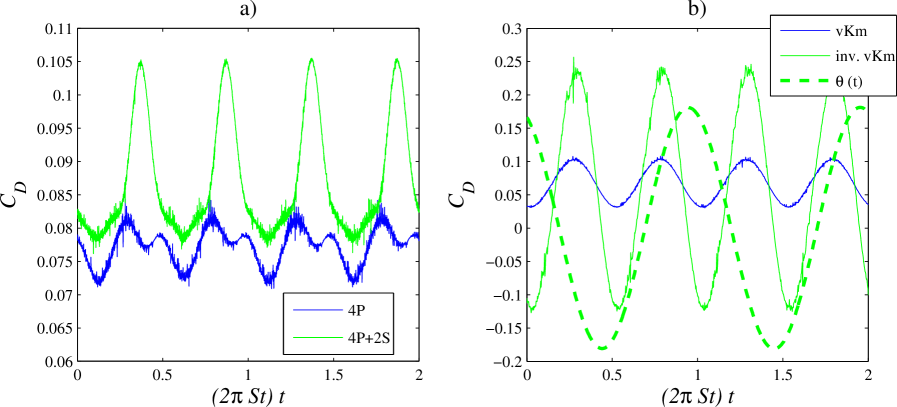
Figure 3: Drag coefficient as function of time for some of the vorticity distributions of Figure 2. a) 4P wake for $St=0.035$ and $A=1.34$ and 4P+2S wake for $St=0.025$ and $A=1.2$ , b) vKm wake for $St=0.12$ and $A=0.98$ and inverted vKm wake for $St=0.12$ and $A=2$. The angle of attack $\theta(t)$ of the foil is shown in (b) for the inverted vKm case.

In Figure 4 it is shown the mean drag coefficient $\langle C_{D}\rangle$ and the difference between $\langle C_{D}\rangle$ and the norm of its Fourier decomposition $C_{DA}$, as a function of the product $StA$. For a sinusoidal $C_{D}$, $\langle C_{D}\rangle-C_{DA}$ is the minimum value of $C_{D}$.

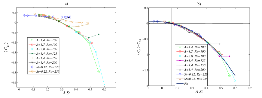
Figure 4: a) Mean drag coefficient $\langle C_{D}\rangle$ and b) $\langle C_{D}\rangle-C_{DA}$ as functions of the $StA$. The lines connecting points mean that either $A$ or $St$ were kept constant as marked. The last two experiments correspond to the parameters used in Schnipper et al. (2009) and Godoy-Diana et al. (2008), respectively. $C=4$ when $Re=255$ and $C=6$ in the rest of the cases.

Figure 4(a) shows that the mean drag decreases monotonically and becomes negative, as $StA$ increases for the cases where $Re<150$. Numerical experiments with higher $Re$ show that $\langle C_{D}\rangle$ decreases and can be negative but starts growing beyond certain value of $StA$. These observations suggest that for a given imposed flow $U$, to which $Re$ is related, there is a critical flapping frequency beyond which the mean drag starts growing. We could not confirm this idea for the cases where $Re<150$ because the numerical model became unstable for high flapping frequencies.

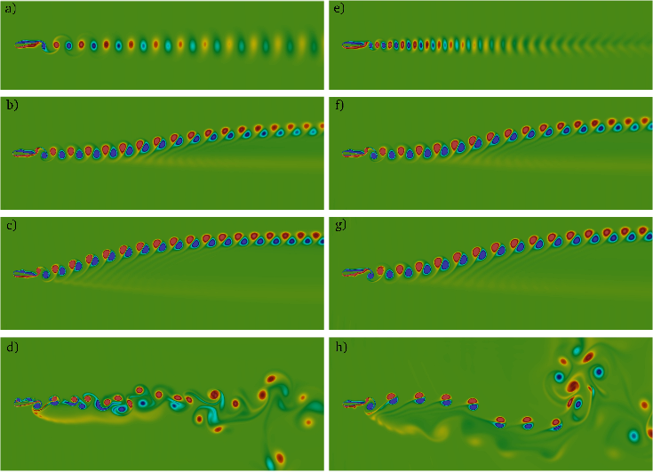
Figure 5: Evolution of the wake for $Re=100$ and $C=6$. a) $StA=0.21$, b) $StA=0.42$, c) $StA=0.49$, d) $StA=0.56$, e) $StA=0.21$, f) $StA=0.42$, g) $StA=0.51$ and h) $StA=0.6$. In the left column the dimensionless amplitude was keep fixed at $A=1.4$ and, in the right column, the Strouhal number was keep fixed at $S=0.3$. Figures show the region of interest within the computational domain. Colours represent positive (red) and negative (blue) vorticity.

Figure 4(b) shows that the minimum of $C_{D}$ crosses zero at $StA\sim 0.16$ regardless of the values of $Re$ and $C$ used. The numerical experiments show that below this value of $StA$ vortices at the wake corresponds to the vKm wake type, but can be combinations of 2S and 2P patterns when $St$ is small. The inverted vKm is found when $StA>0.16$ (see figures 2(b), 5(a) and 5(e)). Figure 4(b) shows that all cases collapse approximately on a single curve given by the fit

$$\langle C_{D}\rangle-C_{DA}=-6.25(StA)^{2.5}+0.066.$$ (5)

For $\mbox{{Re}}=220$ and $C=6$, the wake remains symmetric with a positive value of $\langle C_{D}\rangle$ for all values of $StA$ explored by  Schnipper et al. (2009). The evolution of the wake as function of $A$ and $St$, starting form a vKm wake, is shown in figure 5 for $Re=100$. Beyond the inverted vKm transition, for $StA>0.28$, the wake is deflected from the horizontal centre line and $\langle C_{D}\rangle$ becomes negative. The results shown that the distance between the tail of the foil and the point of deflection seems to decrease as $StA$ increases, in agreement with the numerical simulations made by Deng and Caulfield (2015) (see figures 5(b), (c), (f) and (g)). For $Re=255$, the performed simulations shown that the wake deflects when $StA>0.23$, in good agreement with the 3D experimental observations of Godoy-Diana et al. (2008) and the numerical simulations of He et al. (2012) and Deng and Caulfield (2015).

The direction of deflection is related with the initial condition, and a downwards deflection was found when changing the sign of the angle $\theta_{0}\rightarrow-\theta_{0}$. With the set of parameters used by  Godoy-Diana et al. (2008), the simulations showed that the position and angle of deflection can change with time after several vortex shedding periods of observation, this long time behaviour has been observed by Lewin and Haj-Hariri (2003).

The results with $\mbox{{Re}}=100$ at values of $StA\sim 0.5$ show that the wake becomes unstable (see figures 5 (d) and (h)). The vorticity produced by the foil is still periodic but highly asymmetric, with $C_{L}$ showing only even modes while $C_{D}$ showing contribution from both even and odd modes.

4.2 A free flapping foil

The simulations for the free foil were made using similar initial conditions as in the fixed case. After $5\times 10^{4}$ iterations, where the foil was fixed without flapping, the foils is released and starts flapping with the same exponential increase in amplitude as the fixed case. The values of $StA\in[0.1,0.5]$ were chosen in correspondence to patterns beyond the transition to the inverted vKm wake for the fixed case.

A stationary symmetric flow without vortex shedding was observed before the foil was released in all cases. After released, a transient time was observed where the hydrodynamic force changed from a constant value to a periodic function of time. During this time interval, the centre of mass accelerated until it reached an almost uniform motion in the horizontal direction with small transversal oscillations of the order of $D$ (see figures 6(a) and (d)). The centre of mass deviates vertically a small distance from the horizontal centre line during the transient, probably related to the deflection of the wake.

The centre of mass velocity is a periodic function of time, the horizontal component oscillates around a constant value that is a fraction of the velocity of the free stream ($U=1$ in dimensionless units) with an amplitude that is negligible, hence the swimming velocity is practically constant as shown in figures 6 (a) and (b). The observed amplitude of oscillation of $C_{L}$ is ten times bigger than that of $C_{D}$, which produces a more appreciable oscillation in the vertical direction (see Figures 6 (d)-(f)).

As $StA$ is increased, $V_{x}$ diminishes until it becomes negative and the foil swims upstream. The mean drag becomes very small, $\langle C_{D}\rangle\sim 10^{-4}$ in all cases observed, which is consistent with an almost uniform motion observed at long times in other swimmers (Chisholm et al., 2016; Kern and Koumoutsakos, 2006). Figure 6 (c) shows that minimum values of $C_{D}$ (maximum thrust) are reached little after extremal values of the angle of attack of the foil, suggesting that swimming is not produced by pushing fluid but by a suction mechanism resemblant of that observed by Gemmell et al. (2015) in efficient animal swimming.

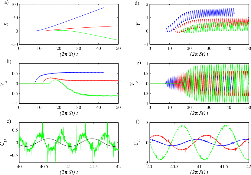
Figure 6: Dynamics of the centre of mass of the foil for $A=1.7$, a) horizontal position $X(t)$, b) horizontal velocity $V_{x}(t)$, c) Drag coefficient $C_{D}(t)$, d) vertical position $Y(t)$ , e) vertical velocity $V_{y}(t)$ and f) Lift coefficient $C_{L}(t)$. (Blue) $St=0.2$, (red) $St=0.3$ and (green) $St=0.45$ . The black line in (c) shows the angle of attack $\theta(t)$.

The wake behind the foil in this region corresponds to a inverted asymmetric vKm wake. When $V_{x}$ is positive (figure 7-(a)) the angle of deflection of the wake seems to be smaller than those observed in the fixed foil cases of similar $StA$ values (see figures 2 (b) and (f)). As $StA$ is increased and $V_{x}$ becomes negative (figure 7-(b)), the deflection of the wake is swept away and becomes symmetric and much longer than the wakes of foils unable to swim upstream. The parameter values for the free foil swimming upstream correspond to the unstable wake for the fixed case (see figure 5-(h)), a P+S mode as seen in figure 8(a). Figure 8 shows how vortical structures at the foil’s surface produce by fixed foil of unsteady wake are larger than those produced by the upstream swimming foil. Probably, the momentum produced by the foil, enough to swim upstream when released, competes with that of the stream to produce the instability.

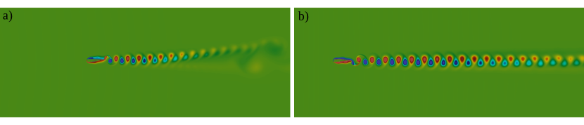
Figure 7: Vorticity distribution for a moving flapping foil for $C=6$, $A=2.0$ and $Re=100$. Colours represent positive (red) and negative (blue) vorticity. a) $St=0.2$ and $V_{x}>0$. b) $St=0.3$ and $V_{x}<0$, the foil swims upstream. Figures show the complete computational domain.

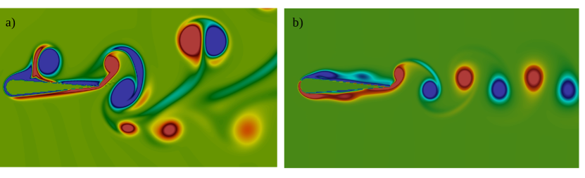
Figure 8: Close up view of the vorticity generated by the foil for $Re=100$, $St=0.3$, and $A=2$. (a) Fixed foil of figure 5-(h) that shows a P+S wake. (b) Free foil of figure 7-(b) that shows an inverted vKm wake.

5 Conclusions

In this work numerical results on the two-dimensional incompressible viscous flow around a flapping foil are presented. Both a fixed and a free flapping foil were considered. The flow field was computed using a lattice Boltzmann model that includes a procedure for moving internal boundaries with arbitrary geometry. Thus allowing the computation of the translational motion of a free foil due to hydrodynamic forces. Numerical results were compared with experiments on soap films (Schnipper et al., 2009) and on wind tunnels (Godoy-Diana et al., 2008).

The numerical simulations show that the transition between the vKm wake and the inverted vKm wake on a fixed flapping foil is found when the flapping Strouhal number $StA\sim 0.16$ and coincides with the minimum value of the horizontal hydrodynamic force on the foil crossing zero. When $St\lesssim 0.16$ the wake can be a 2S (vKm) or 2P. Above this value the wake corresponds to an inverted vKm that deflects as $StA$ increases and the mean horizontal hydrodynamic force becomes negative.

Whenever $\langle C_{D}\rangle$ is a decreasing function of $StA$, there is a universal behaviour for all $Re$ and $C$ explored, with a power law fit given by equation (5). This result can be related with the narrow range of $ASt$ where many mammals swims Taylor et al. (2003). Results suggest that above a certain value of the flapping frequency the drag exerted on the foil starts growing probably producing a flapping foil unable to swim upstream if released.

The cases studied for a flapping foil free of translational motion always reached an almost uniform horizontal speed with a drag coefficient value practically zero. As flapping frequency increases the horizontal velocity becomes negative (upstream motion) and the deflected portion of the wake is swept away. Upstream swimming produces long, symmetric and inverted vKm wakes, and is observed beyond the vKm wake transition, when the fixed foil’s wake becomes unstable. Maximum thrust is observed close to maximal values of the foil’s angle of attack, suggesting swimming through a suction mechanism.

Partial support from project UNAM-PAPIIT-IN115216 and IN115316 is acknowledged. Authors thank Dr. Eduardo Ramos and Dr. Raúl Rechtman for their support.

References

- Anderson et al. (1998) J. M. Anderson, K. Streitlien, D. S. Barrett, and M. S. Triantafyllou. Oscillating foils of high propulsive efficiency. J. Fluid Mech., 360:41–72, 1998.
- Chisholm et al. (2016) N. G. Chisholm, D. Legendre, E. Lauga, and A. S. Khair. A squirmer across Reynolds numbers. J. Fluid Mech., 796:233–256, 2016.
- Clausen et al. (2010) J. R. Clausen, D. A. Reasor, and C. K. Aidun. Parallel performance of a lattice-Boltzmann/finite element cellular blood flow solver on the IBM Blue Gene/P architecture. Comp. Phys. Comm., 181(6):1013–1020, 2010.
- Deng and Caulfield (2015) J. Deng and C. P. Caulfield. Three-dimensional transition after deflection behind a flapping foil. Phys. Rev. E, 91:043017, 2015.
- Dong et al. (2006) H. Dong, R. Mitall, and F. M. Najjar. Wake topology and hydrodynamic performance of low-aspect-ratio flapping foils. J. Fluid Mech., 566:309–343, 2006.
- Gemmell et al. (2015) B. J. Gemmell, S. P. Colin, J. H. Costello, and J. O. Dabiri. Suction-based propulsion as a basis for efficient animal swimming. Nature Comm., 6:8790, 2015.
- Godoy-Diana et al. (2008) R. Godoy-Diana, J.-L. Aider, and J. E. Wesfreid. Transitions in the wake of a flapping foil. Phys. Rev. E, 77:016308, 2008.
- Guo and Zheng (2002) Z. Guo and C. Zheng. An extrapolation method for boundary conditions in lattice Boltzmann method. Phys. Fluids, 14(6):2007–2010, 2002.
- He et al. (2012) G.-Y. He, Q. Wang, X. Zhang, and S.-G. Zhang. Numerical analysis on transitions and symmetry-breaking in the wake of a flapping foil. Acta Mech. Sin., 28(6):1551–1556, 2012.
- He et al. (1998) X. He, S. Chen, and G. D. Doolen. A Novel Thermal Model for the Lattice Boltzmann Method in Incompressible Limit. Journal of Computational Physics, 146:282–300, 1998.
- Kármán and Burgers (1935) T. v. Kármán and J. M. Burgers. General aerodynamic theory – perfect fluids. Dover Publications, 1963, 1935.
- Kern and Koumoutsakos (2006) S. Kern and P. Koumoutsakos. Simulations of optimized anguilliform swimming. J. Exp. Biol., 209:4841–4857, 2006.
- Lewin and Haj-Hariri (2003) G. C. Lewin and H. Haj-Hariri. Modelling thrust generation of a two-dimensional heaving airfoil in a viscous flow. J. Fluid Mech., 492:339–362, 2003.
- Mandujano and Rechtman (2008) F. Mandujano and R. Rechtman. Termal levitation. J. Fluid Mech., 606:105–114, 2008.
- Mei et al. (2002) R. Mei, D. Yu, W. Shyy, and L. Luo. Force evaluation in the lattice Boltzmann method involving curved geometry. Phys. Rev. E, 64:041203, 2002.
- Schnipper et al. (2009) T. Schnipper, A. Andersen, and T. Bohr. Vortex wakes of a flappig foil. J.Fluid Mech., 633:411–423, 2009.
- Taylor et al. (2003) G. K. Taylor, R. L. Nudds, and A. L. R. Thomas. Flying and swimming animals cruise at a Strouhal number tuned for high power efficiency. Nature, 425:707–711, 2003.
- Triantafyllou et al. (2000) M. S. Triantafyllou, G. S. Triantafyllou, and D. K. P. Yue. Hydrodynamics of fishlike swimming. Annu. Rev Fluid Mech., 32:33–53, 2000.
- Vorovieff et al. (2002) P. Vorovieff, D. Georgiev, and M. S. Ingber. Onset of the second wake: dependence on the Reynols number. Phys. Fluids, 14(7):53–57, 2002.
- Williamson and Govardhan (2004) C. H. K. Williamson and R. Govardhan. Vortex-induced vibrations. Annu. Rev. Fluid Mech, 36:413–455, 2004.
- Wu et al. (2015) J. Wu, Y. L. Chen, and N. Zhao. Role of induced vortex interaction in a semi-active flapping foil based energy harvester. Phys. Fluids, 27:093601, 2015.
- Wu (1972) T. Y. Wu. Extraction of flow energy by a wing oscillating in waves. J. Ship Res., 16:66–78, 1972.