Codimension-two Bifurcations Induce Hysteresis Behavior and Multistabilities in Delay-coupled Kuramoto Oscillators

Abstract

Hysteresis phenomena and multistability play crucial roles in the dynamics of coupled oscillators, which are now interpreted from the point of view of codimension-two bifurcations. On the Ott-Antonsen’s manifold, complete bifurcation sets of delay-coupled Kuramoto model are derived regarding coupling strength and delay as bifurcation parameters. It is rigorously proved that the system must undergo Bautin bifurcations for some critical values, thus there always exists saddle-node bifurcation of periodic solutions inducing hysteresis loop. With the aid of center manifold reduction method and the Matlab Package DDE-Biftool, the location of Bautin and double Hopf points and detailed dynamics are theoretically determined. We find that, near these critical points, at most four coherent states (two of which are stable) and a stable incoherent state may coexist, and that the system undergoes Neimark-Sacker bifurcation of periodic solutions. Finally, the clear scenarios about the synchronous transition in delayed Kuramoto model are depicted.

I Introduction

The Kuramoto model was established to investigate the phenomenon of collective synchronization of coupled oscillators with slightly different natural frequencies ref1 ; ref2 ; ref3 ; ref4 , which has been widely observed in physics, chemistry and biology article10 ; article10-1 ; article10-2 ; article10-3 ; article10-4 ; article10-5 . Because of the time lag that signal transmits or that the receiver processes the signal, introducing time delay is natural and necessary in many situations ar9 ; ar91 ; ar901 ; ar912 ; ott1 ; ott2 ; wai ; arkd ; niunon . The Kuramoto model with time delay is of the form

$$\dot{\theta}_{i}=\omega_{i}+\frac{k}{N}\sum_{j=1}^{N}\sin[\theta_{j}(t-\tau)-\theta_{i}(t)],i=1,2,\ldots,N$$ (1)

where $\theta_{i}(t)\in[0,2\pi)$ represents the phase of the $i$th oscillator at time $t$. $\omega_{i},i=1,2,\ldots,N$ are natural frequencies drawn from density $g(\omega),\omega\in(-\infty,+\infty)$, and positive $k$ is the coupling strength. In the thermodynamic limit $N\rightarrow\infty$, define a distribution density $f(\omega,\theta,t)$ characterizing the state of the oscillators’ system at time $t$ in frequency $\omega$ and phase $\theta$. Then the complex-valued mean field $r(t)$ is define by

$$r(t)=\int_{-\infty}^{+\infty}\int_{0}^{2\pi}f(\omega,\theta,t)\textrm{e}^{\textrm{i}\theta}\textrm{d}\theta\textrm{d}\omega$$ (2)

describing the degree to which the oscillators are bunched in phase, where $\textrm{i}=\sqrt{-1}$. Write the continuity equation

$$\frac{\partial}{\partial t}f+\frac{\partial}{\partial\theta}\{[\omega+\frac{k}{2\textrm{i}}(\textrm{e}^{-\textrm{i}\theta}r(t-\tau)-\textrm{e}^{\textrm{i}\theta}r^{\ast}(t-\tau))]f\}=0$$ (3)

with $r^{\ast}$ standing for the complex conjugate. Usually we call $r=0$ ($f$ is uniform distribution) the incoherent state, $|r|=1$ ($f$ is Dirac distribution) the completely synchronized state, and $0<|r|<1$ the partially synchronized state (coherence, for short).

Hopf bifurcation research in Kuramoto model is an efficient way to obtain the transition between the incoherence and coherence ott1 ; niuphyD . Coherent states bifurcating from the incoherent state can be modeled by Hopf bifurcations on some low dimensional manifold, such as the widely used Ott-Antonsen’s manifold ott1 . The direction of Hopf bifurcation, subcritical case or supercritical case, then determines different situations of the synchronization transition.

In ar9 the hysteresis loop and subcritical bifurcations are observed in the delay coupled Kuramoto oscillators. Here, when a hysteresis loop is mentioned, we mean that coherent states and incoherent states coexist in the Kuramoto model when the parameter $k$ is less than the Hopf bifurcation value. In niuphyD , the authors have interpreted the appearance of subcritical Hopf bifurcations in the way of normal form analysis. However, a clear boundary between the supercritical and subcritical bifurcations (a degenerated case) has not been theoretically studied yet. In the viewpoint of bifurcation analysis, this may be involved with the Bautin bifurcation with codimension-two (i.e., generalized Hopf bifurcation)guo ; bautin ; bautin1 ; bautin2 . This is a degenerated case we mainly considered in the current paper. Another degenerated case occurs when two Hopf bifurcation coexist, i.e., the double Hopf bifurcation, which is also codimention two and rarely investigated in the Kuramoto model before. It is well-known that double Hopf bifurcation usually provides a system with oscillations on a 2-torus or 3-torus guo ; homs ; kuz through the Neimark-Sacker bifurcation of periodic solutions. To our best knowledge, codimension-two bifurcation (including Bautin and double Hopf bifurcations) approach to dynamical analysis is brand new to investigate delayed Kuramoto model.

Motivated by such considerations, in this paper, we study the Bautin bifurcation and double Hopf bifurcation on the Ott-Antonsen’s manifold ott1 to reveal some delicate dynamics for delay coupled system (1). The rest part of this paper is organized as follows: we first restate the OA manifold reduction method with respect to system (3), and analyze the characteristic equation of the incoherence. Then Bautin bifurcation and double Hopf bifurcation are analyzed with the aid of center manifold reduction method, respectively. Some illustrations are given with the help of the Matlab Package DDE-Biftool, hence a clear bifurcation set is given in the $\tau-k$ plane. The results are also applied to a system of delay-coupled Hindmarsh-Rose neurons. Finally a conclusion part completes this paper.

II OA Manifold Reduction and Stability of the Incoherence

For the readers’ convenience, we first restate the main results about OA manifold reduction of (1) by ott1 . Restrict (3) on the OA manifold

$$\mathcal{M}_{OA}=\left\{f(\theta,\omega,t):f=\frac{g(\omega)}{2\pi}\left\{1+\left[\sum_{n=1}^{\infty}\alpha^{n}(\omega,t)\textrm{e}^{\textrm{i}n\theta}+c.c.\right]\right\}\right\}$$

with c.c. the complex conjugate of the formal terms and $\alpha^{n}(\omega,t)$ the Fourier coefficients. Substituting the Fourier series of $f$ into (3) and after comparing the coefficients of the same harmonic terms, a reduced equation is obtained

$$\dot{\alpha}(\omega,t)=-\textrm{i}\omega\alpha(\omega,t)+\frac{k}{2}r^{\ast}(t-\tau)-\frac{k}{2}r(t-\tau)\alpha^{2}(\omega,t)$$ (4)

Following the OA ansatz ott1 and applying Cauchy’s residue theorem to Eq.(2), we have

$$r(t)=\int_{-\infty}^{+\infty}g(\omega)\alpha^{\ast}(\omega,t)\textrm{d}\omega=\alpha^{\ast}(\omega_{0}-\textrm{i}\Delta,t)$$ (5)

provided that $g(\omega)$ is chosen to be the Lorentzian distribution $g(\omega)=\frac{\Delta}{\pi[(\omega-\omega_{0})^{2}+\Delta^{2}]},~{}-\infty<\omega<+\infty$ with the spreading width $\Delta>0$ and the median value $\omega_{0}>0$.

Putting $\omega=\omega_{0}-\textrm{i}\Delta$ in Eq.(4) yields a reduced functional differential equation Halefde

$$\dot{r}(t)=-(\textrm{i}\omega_{0}+\Delta)r(t)+\frac{k}{2}r(t-\tau)-\frac{k}{2}r^{\ast}(t-\tau)r^{2}(t)$$ (6)

To give the transition from incoherence to coherence, we need to investigate the characteristic equation around the incoherence $r=0$

$$\lambda=-(\textrm{i}\omega_{0}+\Delta)+\frac{k}{2}\textrm{e}^{-\lambda\tau}$$ (7)

Since we are about to study codimension-two bifurcations, regarding $k$ and $\tau$ as bifurcation parameters, we know Eq.(6) undergoes local bifurcation at $r=0$ if (7) has roots with zero real part for some $(k,\tau)$. Noticing the assumption $\omega_{0}\neq 0$, we let $\lambda=\textrm{i}\beta$ with $\beta\neq 0$ be a root of (7), then

$$\begin{array}[]{rcl}\Delta&=&\frac{1}{2}k\cos\tau\beta\\ -\beta-\omega_{0}&=&\frac{1}{2}k\sin\tau\beta\end{array}$$ (8)

which yields

$$\beta^{2}+2\omega_{0}\beta+\Delta^{2}+\omega_{0}^{2}-\frac{k^{2}}{4}=0$$

Obviously, $\beta$ is solved by

$$\beta=\beta_{\pm}=-\omega_{0}\pm\sqrt{\frac{k^{2}}{4}-\Delta^{2}}$$

if $k>2\Delta$ holds. Furthermore, from (8), two sequences of critical values $\tau_{j}^{\pm}(k)$ are defined by

$$\tau_{j}^{+}(k)=\left\{\begin{array}[]{ll}\frac{\arcsin\frac{-2\beta_{+}-2\omega_{0}}{k}-2j\pi}{\beta_{+}},&k^{2}\leq 4(\Delta^{2}+\omega_{0}^{2})\\ \frac{\arcsin\frac{-2\beta_{+}-2\omega_{0}}{k}+2(j+1)\pi}{\beta_{+}},&k^{2}>4(\Delta^{2}+\omega_{0}^{2})\end{array}j=0,1,2,\cdots\right.$$ (9)

and

$$\tau_{j}^{-}(k)=\frac{\arcsin\frac{-2\beta_{-}-2\omega_{0}}{k}-2(j+1)\pi}{\beta_{-}},j=0,1,2,\cdots$$ (10)

This means that (7) has a root $\textrm{i}\beta_{+}$ (or $\textrm{i}\beta_{-}$), if $(\tau,k)=(\bar{\tau},\bar{k})\in\{(\tau,k)|k>2\Delta,\tau=\tau_{j}^{+}{(k)}~{}(\textrm{or}~{}\tau_{j}^{-}(k))\}$. Usually, purely imaginary roots of characteristic equation mean Hopf bifurcation or Bautin bifurcation. The bifurcating periodic solution $r(t)\approx r_{0}\textrm{e}^{\textrm{i}\beta t}$ with small amplitude $r_{0}$ of (6) corresponds to a coherent state of (1). Obtaining precise results requires the normal forms near the critical points.

III Bautin bifurcation

When $k=\bar{k}>2\Delta$, the characteristic equation (7) has a purely imaginary root if $\tau=\bar{\tau}\in\{\tau_{j}^{\pm}(\bar{k}),j=0,1,2,\cdots\}$. In order to obtain the bifurcation results, we need calculate the normal form by using the center manifold reduction method Hassard ; faria ; guo basing on the formal adjoint theory Halefde . It is worthy mentioning that the method of multiple time scales can be also used to obtained normal forms in delay equations naybook ; Yums ; dfmms ; Nay . The two approaches lead to the same normal forms ding , thus we use the center manifold reduction approach here. Normalizing time by $\tau$, we rewrite Eq.(6) as

$$\begin{array}[]{rl}\dot{r}(t)=-\tau(\textrm{i}\omega_{0}+\Delta)r(t)+\frac{k}{2}\tau r(t-1)-\frac{k}{2}\tau r^{\ast}(t-1)r^{2}(t)\end{array}$$ (11)

with a characteristic equation at $r=0$

$$\lambda=-\tau(\textrm{i}\omega_{0}+\Delta)+\tau\frac{k}{2}\textrm{e}^{-\lambda}$$ (12)

Clearly, $\textrm{i}\beta$ is a root of (7) if and only if $\textrm{i}\tau\beta$ is a root of (12). Slightly perturbing $k=\bar{k}+\epsilon$ and $\tau=\bar{\tau}+\delta$, we have the equivalent form of (11)

$$\begin{array}[]{rl}\dot{r}=-(\bar{\tau}+\delta)(\textrm{i}\omega_{0}+\Delta)r+\frac{(\bar{k}+\epsilon)(\bar{\tau}+\delta)}{2}r(t-1)-\frac{(\bar{k}+\epsilon)(\bar{\tau}+\delta)}{2}r^{\ast}(t-1)r^{2}\end{array}$$ (13)

If $(\epsilon,\delta)=(0,0)$, i.e., $(\tau,k)=(\bar{\tau},\bar{k})$, $\textrm{i}\bar{\tau}\beta$ is a root of (12).

For any $\varphi\in C([-1,0],\mathbf{C})$ with $\mathbf{C}$ the space of complex numbers, we define a linear operator

$$L_{\epsilon,\delta}(\varphi)=\int_{-1}^{0}\textrm{d}\eta(\theta,\epsilon,\delta)\varphi(\theta)\\$$

with

$$\eta(\theta,\epsilon,\delta)=\left\{\begin{array}[]{ll}-(\bar{\tau}+\delta)(\textrm{i}\omega_{0}+\Delta)+\frac{(\bar{k}+\epsilon)}{2}(\bar{\tau}+\delta),&\theta=0\\ \frac{(\bar{k}+\epsilon)}{2}(\bar{\tau}+\delta),&\theta\in(-1,0)\\ 0,&\theta=-1\end{array}\right.$$

Meanwhile, for $\varphi\in C^{1}([-1,0],\mathbf{C})$, we define

$$A(\epsilon,\delta)\varphi=\left\{\begin{array}[]{ll}\frac{\textrm{d}\varphi(\theta)}{\textrm{d}\theta},&\theta\in[-1,0)\\ L_{\epsilon,\delta}(\varphi),&\theta=0\end{array}\right.$$

$$F(\epsilon,\delta,\varphi)=-\frac{(\bar{k}+\epsilon)(\bar{\tau}+\delta)}{2}\varphi^{\ast}(-1)\varphi^{2}(0)$$

and

$$R(\epsilon,\delta)\varphi=\left\{\begin{array}[]{ll}0,&\theta\in[-1,0)\\ F(\epsilon,\delta,\varphi),&\theta=0\end{array}\right.$$

Then system (13) can be transformed into an abstract ordinary differential equation

$$\dot{r}_{t}=A(\epsilon,\delta)r_{t}+R(\epsilon,\delta)r_{t}$$ (14)

with $r_{t}=r(t+\theta),\theta\in[-1,0]$.

For $\psi\in C^{1}([-1,0],{\mathbf{C}})$, define the adjoint operator of $A(0,0)$ by

$$\hat{A}\psi=\left\{\begin{array}[]{ll}-\frac{\textrm{d}\psi(s)}{\textrm{d}s},&s\in(0,1]\\ \int_{-1}^{0}\psi(-s)\textrm{d}\eta^{\ast}(\theta,0,0),&s=0\end{array}\right.$$

For $\varphi\in C([-1,0],\mathbf{C})$ and $\psi\in C([0,1],{\mathbf{C}})$, define the bilinear form

$$<\psi,\phi>=\psi^{\ast}(0)\varphi(0)-\int_{\theta=-1}^{0}\int_{\zeta=0}^{\theta}\psi^{\ast}(\zeta-\theta)\textrm{d}\eta(\theta,0,0)\varphi(\zeta)\textrm{d}\zeta$$

We know that $\textrm{i}\bar{\tau}\beta$ is an eigenvalue of $A(0,0)$ and $-\textrm{i}\bar{\tau}\beta$ is an eigenvalue of $\hat{A}$. Suppose $q(\theta)$ and $\hat{q}(s)$ are the corresponding eigenvectors, i.e.,

$$\begin{array}[]{l}A(0,0)q=\textrm{i}\bar{\tau}\beta q,\hat{A}\hat{q}=-\textrm{i}\bar{\tau}\beta\hat{q}\end{array}$$

Letting $q(\theta)=\textrm{e}^{\textrm{i}\beta\bar{\tau}\theta}$, $\hat{q}(s)=\frac{1}{1+\frac{1}{2}\bar{k}\bar{\tau}\textrm{e}^{\textrm{i}\beta\bar{\tau}}}\textrm{e}^{\textrm{i}\beta\bar{\tau}s}$, we have $<\hat{q},q>=1$.

Due to the classical results in Halefde , for $|(\epsilon,\delta)|$ sufficiently small, we use $z(t)$ as complex coordinate on the center manifold in direction $q$, thus $z(t)=<\hat{q},r_{t}>$. Decomposing

$$r_{t}(\theta)=z(t)q(\theta)+W^{(\epsilon,\delta)}(z,z^{\ast},\theta)$$ (15)

with $W^{(\epsilon,\delta)}(z,z^{\ast},\theta)=\sum_{i+j\geq 2}W_{ij}^{(\epsilon,\delta)}(\theta)\frac{1}{i!j!}z^{i}{z^{\ast}}^{j}$. Denote $W^{(0,0)}$ by $W$ and $W_{ij}^{(0,0)}$ by $W_{ij}$ for simplicity. We can calculate

$$\begin{array}[]{rl}\dot{z}(t)&=<\hat{q},\dot{r}_{t}>\\ &=<\hat{q},A(0,0)r_{t}+[A(\epsilon,\delta)-A(0,0)]r_{t}+R(\epsilon,\delta)r_{t}>\\ &=<\hat{A}\hat{q},r_{t}>+<\hat{q},[A(\epsilon,\delta)-A(0,0)]r_{t}>+<\hat{q},R(\epsilon,\delta)r_{t}>\\ &=\textrm{i}\bar{\tau}\beta z(t)+<\hat{q},[A(\epsilon,\delta)-A(0,0)]r_{t}>+\hat{q}^{\ast}(0)F(\epsilon,\delta,r_{t})\end{array}$$ (16)

Rewrite (16) as

$$\dot{z}(t)=\textrm{i}\bar{\tau}\beta z(t)+<\hat{q},[A(\epsilon,\delta)-A(0,0)]r_{t}>+g(z,z^{\ast})$$ (17)

then we Taylor expand $g(z,z^{\ast})=\hat{q}^{\ast}(0)F(\epsilon,\delta,r_{t}):=\sum_{i+j\geq 2}g_{ij}\frac{1}{i!j!}z^{i}{z^{\ast}}^{j}$. According to the results about normal form with imaginary roots guo ; Wiggins2 , we have the normal form is

$$\dot{z}=\textrm{i}\bar{\tau}\beta z+l_{0}(\epsilon,\delta)z+\frac{1}{2}l_{1}(\epsilon,\delta)z^{2}z^{\ast}+\frac{1}{12}l_{2}(\epsilon,\delta)z^{3}{z^{\ast}}^{2}+h.o.t.$$

with

$$l_{0}(\epsilon,\delta)=\frac{1}{1+\frac{1}{2}\bar{k}\bar{\tau}\textrm{e}^{-\textrm{i}\beta\bar{\tau}}}\left[\frac{1}{2}\bar{\tau}\textrm{e}^{-\textrm{i}\beta\bar{\tau}}\epsilon+\left(-\Delta+\frac{1}{2}\bar{k}\textrm{e}^{-\textrm{i}\beta\bar{\tau}}-\textrm{i}\omega_{0}\right)\delta\right]$$

Obviously, $(Re\frac{\partial{l_{0}}}{\partial\epsilon},Re\frac{\partial{l_{0}}}{\partial\delta})\neq 0$ yields the satisfaction of transversality condition. The first and second Lyapunov coefficients at $\epsilon=\delta=0$ are $Rel_{1}(0,0)=\frac{Img_{20}g_{11}}{\bar{\tau}|\beta|}+{Reg_{21}}$ and

$$\begin{array}[]{rl}&12Rel_{2}(0,0)=Re{g_{32}}\\ &~{}~{}+\frac{1}{\bar{\tau}|\beta|}Im\left\{g_{20}\bar{g}_{31}-g_{11}(4g_{31}+3\bar{g}_{22})-\frac{1}{3}g_{02}(g_{40}+\bar{g}_{13})-g_{30}g_{12}\right\}\\ &~{}~{}+\frac{1}{\bar{\tau}^{2}\beta^{2}}Re\left\{g_{20}\left[\bar{g}_{11}(3g_{12}-\bar{g}_{30})+g_{02}\left(\bar{g}_{12}-\frac{1}{3}g_{30}\right)+\bar{g}_{02}g_{03}\right]\right\}\\ &~{}~{}+\frac{1}{\bar{\tau}^{2}\beta^{2}}Re\left\{g_{11}\left[\bar{g}_{02}\left(\frac{5}{3}\bar{g}_{30}+3g_{12}\right)+\frac{1}{3}g_{02}\bar{g}_{03}-4g_{11}g_{30}\right]\right\}\\ &~{}~{}+\frac{3}{\bar{\tau}^{2}\beta^{2}}Im\{g_{20}g_{11}\}Im\{g_{21}\}+\frac{1}{\bar{\tau}^{3}|\beta|^{3}}Im\{g_{11}\bar{g}_{02}[\bar{g}_{20}^{2}-3\bar{g}_{20}g_{11}-4g_{11}^{2}\}\\ &~{}~{}+\frac{1}{\bar{\tau}^{3}|\beta|^{3}}Im\left\{g_{11}g_{20}\right\}[3Re\{g_{11}g_{20}\}-2|g_{02}|^{2}]\end{array}$$

Due to the lack of second order terms in $F(\epsilon,\delta,\varphi)$, simply we have

$$g_{20}=g_{11}=g_{02}=0,~{}g_{21}=-\frac{\bar{k}\bar{\tau}}{2}\frac{\textrm{e}^{\textrm{i}\beta\bar{\tau}}}{1+\frac{1}{2}\bar{k}\bar{\tau}\textrm{e}^{-\textrm{i}\beta\bar{\tau}}}$$

$$g_{30}=g_{12}=g_{03}=g_{04}=0,~{}g_{40}=-\frac{\bar{k}\bar{\tau}}{2}\frac{1}{{1+\frac{1}{2}\bar{k}\bar{\tau}\textrm{e}^{-\textrm{i}\beta\bar{\tau}}}}(w_{02}^{\ast}(-1))$$

$$g_{31}=-\frac{\bar{k}\bar{\tau}}{2}\frac{1}{{1+\frac{1}{2}\bar{k}\bar{\tau}\textrm{e}^{-\textrm{i}\beta\bar{\tau}}}}(2\textrm{e}^{-\textrm{i}\beta\bar{\tau}}w_{20}(0)+w_{11}^{\ast}(-1))$$

$$g_{22}=-\frac{\bar{k}\bar{\tau}}{2}\frac{1}{{1+\frac{1}{2}\bar{k}\bar{\tau}\textrm{e}^{-\textrm{i}\beta\bar{\tau}}}}(2\textrm{e}^{-\textrm{i}\beta\bar{\tau}}w_{11}(0)+w_{20}^{\ast}(-1))$$

$$g_{13}=-\frac{\bar{k}\bar{\tau}}{2}\frac{1}{{1+\frac{1}{2}\bar{k}\bar{\tau}\textrm{e}^{-\textrm{i}\beta\bar{\tau}}}}(2\textrm{e}^{-\textrm{i}\beta\bar{\tau}}w_{02}(0))$$

and

$$g_{32}=-\frac{\bar{k}\bar{\tau}}{2}\frac{1}{{1+\frac{1}{2}\bar{k}\bar{\tau}\textrm{e}^{-\textrm{i}\beta\bar{\tau}}}}(w_{21}^{\ast}(-1)+2w_{20}^{\ast}(-1)w_{20}(0)+2w_{02}^{\ast}(-1)w_{02}(0)+2\textrm{e}^{-\textrm{i}\beta\bar{\tau}}w_{21}(0))$$

Plugging (15) and (16) into (14), we have

$$\dot{W}=\left\{\begin{array}[]{l}AW-\hat{q}^{\ast}(0)F(0,0,r_{t})q(\theta),-1\leq\theta<0\\ AW-\hat{q}^{\ast}(0)F(0,0,r_{t})q(\theta)+F(0,0,r_{t}),\theta=0\end{array}\right.$$ (18)

In fact $\dot{W}=W_{z}\dot{z}+W_{z^{\ast}}\dot{z}^{\ast}$, then balancing the coefficients $z$ and $z^{\ast}$ in (18), we have some differential equations and initial conditions, by solving which we obtain the unknown $w_{20},w_{02},w_{11}$ and $w_{21}$ above. Here we omit the tedious expressions (these calculations can be found in guo ; bautin1 ; bautin2 ) and only give the final expressions of $l_{1}(0,0)$ and $l_{2}(0,0)$ by running a computer program,

$$l_{1}(0,0)=-\frac{\bar{k}\bar{\tau}}{2}Re\frac{\textrm{e}^{\textrm{i}\beta\bar{\tau}}}{1+\frac{1}{2}\bar{k}\bar{\tau}\textrm{e}^{-\textrm{i}\beta\bar{\tau}}},l_{2}(0,0)=-3\bar{k}\bar{\tau}Re\frac{1}{1+\frac{1}{2}\bar{k}\bar{\tau}\textrm{e}^{-\textrm{i}\beta\bar{\tau}}}$$

Using the fundamental results in homs ; kuz ; Wiggins2 , we have

      Theorem 1

At the critical point $(\bar{k},\bar{\tau})$, if Re$l_{1}(0,0)\neq 0$, then system (6) undergoes a Hopf bifurcation, which is supercritical if Re$l_{1}(0,0)<0$ and subcritical if Re$l_{1}(0,0)>0$. If Re$l_{1}(0,0)=0$, and Re$l_{2}(0,0)\neq 0$, then system (6) undergoes a Bautin bifurcation.

In fact Sgn Re $l_{1}(0,0)=$ Sgn $-\Delta-2\bar{\tau}\Delta^{2}+\frac{\bar{\tau}}{4}{\bar{k}}^{2}$, thus we have

      Corollary 1

For any $\Delta>0,\omega_{0}>0$, system (6) always undergoes Bautin bifurcations at some $(\bar{\tau},\bar{k})$. There always exists a curve of saddle-node bifurcations of periodic orbits originating from each Bautin point, which gives birth to the hysteresis loop in the delay-coupled Kuramoto model (1). A generic result is shown in Figure 1.

Proof: In the $\tau-k$ plane, we know Hopf bifurcation appears for all $k>2\Delta$. The curve $-\Delta-2\tau\Delta^{2}+\frac{\tau}{4}{k}^{2}=0$ admits $k=\sqrt{{4\Delta}/{\tau}+8\Delta^{2}}$, which is a monotone decreasing function of $\tau$, and approximates to $k=2\sqrt{2}\Delta>2\Delta$ as $\tau\rightarrow\infty$, and to $+\infty$ as $\tau\rightarrow 0$. Thus we know there must exist some intersecting points between the Hopf curves and the critical curve $-\Delta-2\tau\Delta^{2}+\frac{\tau}{4}{k}^{2}=0$, i.e., Bautin points. Moreover, we have Re$l_{2}(0,0)=$Re$[1+\bar{\tau}(\textrm{i}\beta+\textrm{i}\omega_{0}+\Delta)]^{-1}>0$ from (12). The rest results are direct applications of the classical results in homs .

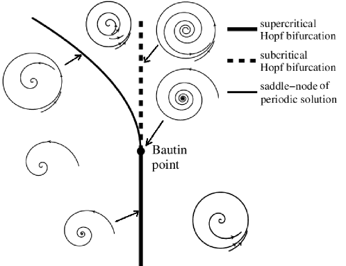
Figure 1: Bifurcation sets around a generic Bautin point with Re$l_{2}(0,0)<0$.

IV Double Hopf Bifurcation

Usually, two Hopf bifurcation curves on the $\tau-k$ plane intersect, leaving the system with some double Hopf points guo .

Still denoting these double Hopf points by $(\bar{\tau},\bar{k})$, we set $(\tau,k)=(\bar{\tau},\bar{k})+(\epsilon,\delta)$ to proceed bifurcation analysis. We assume in this case that $\textrm{i}\bar{\tau}\alpha$ and $\textrm{i}\bar{\tau}\beta$ are eigenvalues of $A(0,0)$. Hence $-\textrm{i}\bar{\tau}\alpha$ and $-\textrm{i}\bar{\tau}\beta$ are eigenvalues of $\hat{A}$. Suppose $q_{1}(\theta),q_{2}(\theta)$ and $\hat{q}_{1}(s),\hat{q}_{2}(s)$ are the corresponding eigenvectors, i.e.,

$$A(0,0)q_{1}=\textrm{i}\bar{\tau}\alpha q,\hat{A}\hat{q}_{1}=-\textrm{i}\bar{\tau}\alpha\hat{q},A(0,0)q_{2}=\textrm{i}\bar{\tau}\beta q,\hat{A}\hat{q}_{2}=-\textrm{i}\bar{\tau}\beta\hat{q}$$

Let $q_{1}(\theta)=\textrm{e}^{\textrm{i}\alpha\bar{\tau}\theta}$, $q_{2}(\theta)=\textrm{e}^{\textrm{i}\beta\bar{\tau}\theta}$ and $\hat{q}_{1}(s)=D_{1}^{\ast}\textrm{e}^{\textrm{i}\alpha\bar{\tau}s}$, $\hat{q}_{2}(s)=D_{2}^{\ast}\textrm{e}^{\textrm{i}\beta\bar{\tau}s}$, $D_{1}=\frac{1}{1+\frac{1}{2}\bar{k}\bar{\tau}\textrm{e}^{-\textrm{i}\alpha\bar{\tau}}},D_{2}=\frac{1}{1+\frac{1}{2}\bar{k}\bar{\tau}\textrm{e}^{-\textrm{i}\beta\bar{\tau}}}$, then we have $<\hat{q}_{1},q_{1}>=<\hat{q}_{2},q_{2}>=1$ and $<\hat{q}_{1},q_{2}>=<\hat{q}_{2},q_{1}>=0$.

Using $z_{1}(t)$ and $z_{2}(t)$ as complex coordinates on the center manifold for small $|(\epsilon,\delta)|$, we have $z_{1}(t)=<\hat{q}_{1},r_{t}>$, $z_{2}(t)=<\hat{q}_{2},r_{t}>$. Then

$$\begin{array}[]{rl}\dot{z}_{1}(t)&=<\hat{q}_{1},\dot{r}_{t}>\\ &=<\hat{q}_{1},A(\epsilon,\delta)r_{t}+R(\epsilon,\delta)r_{t}>\\ &=<\hat{A}\hat{q}_{1},r_{t}>+<\hat{q}_{1},[A(\epsilon,\delta)-A(0,0)])r_{t}>+<\hat{q}_{1},R(\epsilon,\delta)r_{t}>\\ &=\textrm{i}\bar{\tau}\alpha z_{1}(t)+<\hat{q}_{1},[A(\epsilon,\delta)-A(0,0)])r_{t}>+\hat{q}_{1}^{\ast}(0)F(\epsilon,\delta,r_{t})\end{array}$$

$$\begin{array}[]{rl}\dot{z}_{2}(t)&=<\hat{q}_{2},\dot{r}_{t}>\\ &=<\hat{q}_{2},A(\epsilon,\delta)r_{t}+R(\epsilon,\delta)r_{t}>\\ &=<\hat{A}\hat{q}_{2},r_{t}>+<\hat{q}_{2},[A(\epsilon,\delta)-A(0,0)])r_{t}>+<\hat{q}_{2},R(\epsilon,\delta)r_{t}>\\ &=\textrm{i}\bar{\tau}\beta z_{2}(t)+<\hat{q}_{2},[A(\epsilon,\delta)-A(0,0)])r_{t}>+\hat{q}_{2}^{\ast}(0)F(\epsilon,\delta,r_{t})\end{array}$$

Letting $r_{t}(\theta)=z_{1}(t)q_{1}(\theta)+z_{2}(t)q_{2}(\theta)+W(z,z^{\ast},\theta)$, and following the same method given in guo , if the nonresonant condition

$$|\alpha|\neq 3|\beta|,3|\alpha|\neq|\beta|$$ (19)

is satisfied, the third order normal form near a double Hopf point is derived

$$\begin{array}[]{lll}\dot{z}_{1}&=&a_{11}\epsilon z_{1}+a_{12}\delta z_{1}+c_{11}z_{1}^{2}z_{1}^{\ast}+c_{12}z_{1}z_{2}z_{2}^{\ast}\\ \dot{z}_{2}&=&a_{21}\epsilon z_{2}+a_{22}\delta z_{2}+c_{21}z_{1}z_{1}^{\ast}z_{2}+c_{22}z_{2}^{2}z_{2}^{\ast}\end{array}$$

where

$$\begin{array}[]{l}a_{11}=\frac{1}{2}D_{1}\bar{\tau}\textrm{e}^{-\textrm{i}\alpha\bar{\tau}},a_{12}=D_{1}\left(-\Delta+\frac{1}{2}\bar{k}\textrm{e}^{-\textrm{i}\alpha\bar{\tau}}-\textrm{i}\omega_{0}\right)\\ c_{11}=-\frac{1}{2}D_{1}\bar{k}\bar{\tau}\textrm{e}^{\textrm{i}\alpha\bar{\tau}},c_{12}=-\frac{1}{2}D_{1}\bar{k}\bar{\tau}\textrm{e}^{\textrm{i}\beta\bar{\tau}}\\ a_{21}=\frac{1}{2}D_{2}\bar{\tau}\textrm{e}^{-\textrm{i}\beta\bar{\tau}},a_{22}=D_{2}\left(-\Delta+\frac{1}{2}\bar{k}\textrm{e}^{-\textrm{i}\beta\bar{\tau}}-\textrm{i}\omega_{0}\right)\\ c_{21}=-\frac{1}{2}D_{2}\bar{k}\bar{\tau}\textrm{e}^{\textrm{i}\alpha\bar{\tau}},c_{22}=-\frac{1}{2}D_{2}\bar{k}\bar{\tau}\textrm{e}^{\textrm{i}\beta\bar{\tau}}\end{array}$$

After rescaling $\epsilon_{1}=\textrm{Sign}(\textrm{Re}c_{11})$, $\epsilon_{2}=\textrm{Sign}(\textrm{Re}c_{22})$, $r_{1}=|z_{1}|,$ $r_{2}=|z_{2}|$, $t\rightarrow t\epsilon_{1}$ we have the amplitude equation

$$\begin{array}[]{lll}\dot{r}_{1}&=&r_{1}(c_{1}+r_{1}^{2}+b_{0}r_{2}^{2})\\ \dot{r}_{2}&=&r_{2}(c_{2}+c_{0}r_{1}^{2}+d_{0}r_{2}^{2})\end{array}$$ (20)

with

$$\begin{array}[]{l}c_{1}=\epsilon_{1}\textrm{Re}a_{11}\epsilon+\epsilon_{1}\textrm{Re}a_{12}\delta,c_{2}=\epsilon_{1}\textrm{Re}a_{21}\epsilon+\epsilon_{1}\textrm{Re}a_{22}\delta\\ b_{0}=\frac{\epsilon_{1}\epsilon_{2}\textrm{Re}c_{12}}{\textrm{Re}c_{22}},c_{0}=\frac{\textrm{Re}c_{21}}{\textrm{Re}c_{11}},d_{0}=\epsilon_{1}\epsilon_{2}\end{array}$$

Applying the results in homs , Eq.(20) has twelve distinct types of unfoldings, distinguished by the signs of $b_{0},~{}c_{0},~{}d_{0}$ and $d_{0}-b_{0}c_{0}$. In the coming section, we will give a numerical example to show the detailed bifurcation sets near a double Hopf point.

V Numerical Experiments

In this section, some illustrations are given to support the theoretical results obtained about Bautin and double Hopf bifurcations in (11). Meanwhile the Kuramoto model (1) is also simulated. The existence of multistabilities is observed in a delay-coupled system of Hindmarsh-Rose neurons.

V.1 Simulations near the Bautin bifurcation

When $\omega_{0}=3$ and $\Delta=0.1$, by using (9) and (10) we draw the Hopf bifurcation values by thick black curves shown in Figure 2(a). The red dashed curve stands for $-\Delta-2\tau\Delta^{2}+\frac{\tau}{4}k^{2}=0$, above which the Hopf bifurcation is subcritical and below which the bifurcation is supercritical. This is a theoretical proof of FIG.4 in ar9 .

Four Bautin bifurcation points and two double Hopf points are marked by B${}_{1}-$B₄ and HH${}_{1}-$HH₂. The blue, thin curves stands for the saddle-node bifurcation of periodic solutions originating from Bautin points by using DDE-Biftool ddebif1 ; ddebif2 .

In fact, at B₁, some calculations yield $k=0.9146,\tau=0.5288$, Re$l_{1}(0,0)=0$ and Re$l_{2}(0,0)=-0.1619<0$. At B₂, we have $k=0.5819,\tau=1.5469$, Re$l_{1}(0,0)=0$ and Re$l_{2}(0,0)=-0.0679<0$. Thus from Corollary 1 and Figure 1 we know there exists a region near each Bautin points (see Figure2(b,d)), where a stable equilibrium, a stable periodic orbit and an unstable periodic orbit coexist (Regions VIII or X).

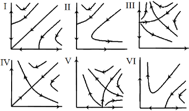
a)b)
c)d)

Figure 2: (color online) a) Hopf bifurcation curves (black, thick) of Eq.(6) are shown in the $k-\tau$ plane for $\omega_{0}=3$ and $\Delta=0.1$. HH${}_{1}-$HH₂ are double Hopf points. B${}_{1}-$B₄ are Bautin points. Blue (thin) curves stand for saddle-node bifurcation of periodic orbits. Red (dashed) curve stands for the line $-\Delta-2\tau\Delta^{2}+\frac{\tau}{4}k^{2}=0$, above which Hopf bifurcations are subcritical and below which Hopf bifurcations are supercritical. b) figure a) is zoomed in the region $[0.5,1.6]\times[0.5,4]$ and the red dash-dotted curves stand for the Neimark-Sacker bifurcations. c) local phase portraits for parameters in regions I-VI of b) in polar coordinates $r_{1}$ and $r_{2}$ of Eq.(20). d) phase portraits for parameters in regions VII-XI.

V.2 Simulations near the double Hopf bifurcation

Fixing $\omega_{0}=3,\Delta=0.1$, at the double Hopf point HH₁, we have $k=3.1286$, $\tau=1.0472$, and two imaginary roots of the characteristic equation (12) are $\textrm{i}\alpha=-\textrm{i}1.4389$, $\textrm{i}\beta=-\textrm{i}4.5611$, which means the nonresonant condition (19) is fulfilled. By using the normal form method given in Section 4, we have $c_{1}=0.2289\epsilon-0.6042\delta$, $c_{2}=1.9153\delta+0.2289\epsilon$, $d_{0}=1$, $b_{0}=c_{0}=-1.0905$. This corresponds to the case IVb given in Section 7.5 of homs , and there exists two Neimark-Sacker bifurcation curves of periodic solutions (torus bifurcation) originating from HH₁. For sufficiently small $\epsilon$ and $\delta$, the two Neimark-Sacker bifurcation curves can be calculated locally, by $c_{2}=c_{0}c_{1}$ and $c_{2}=c_{1}/b_{0}$, which are $\epsilon=-2.6253\delta$ and $\epsilon=-3.1018\delta$.

Using the DDE-Biftool, we draw the global Neimark-Sacker bifurcation curves in Figure 2(b) in red dash-dotted curves, above which system (6) exhibits unstable oscillations on 2-torus. In Figure 2(c), we give a complete local (near the origin) bifurcation sets in polar coordinates $r_{1}$ and $r_{2}$ of Eq.(20) homs . Clearly, in regions III, IV and V, there exist solutions oscillating around both $r_{1}$-axis and $r_{2}$-axis.

So far, we have studied the delay coupled Kuramoto oscillators on the OA manifold from the point of view of Bautin and double Hopf bifurcation analysis. Through some elaborative bifurcation analysis, we give a complete bifurcation set in the plane of delay and coupling strength. To sum up, we can give a result in Table 1, where the stability of $r=0$, number of stable periodic orbits, unstable periodic orbits or 2-torus of Eq.(6) are shown in the regions I-XI on $\tau-k$ plane. With respect to the Kuramoto model, we recall that $r=0$ represents the incoherence, the periodic solutions stands for the coherent states. Thus we obtain clear scenarios about the synchronous transition of delayed Kuramoto model (1).

Table 1: Stability of $r=0$ (s for stable, u for unstable), number of stable periodic orbits, unstable periodic orbits and 2-torus of Eq.(6) for parameters in I-XI.

	I	II	III	IV	V	VI	VII	VIII	IX	X	XI
$r=0$	s	u	u	u	u	u	u	s	s	s	u
stable PO	2	2	2	2	2	2	1	1	0	1	1
unstable PO	2	1	1	0	1	1	0	1	0	1	0
2-torus	0	0	1	1	1	0	0	0	0	0	0

V.3 Simulations of the Kuramoto model

Now, some illustrations by integrating the Kuramoto model (1) are given as comparisons with the reduced model (6).

Choosing $\omega_{0}=3$, $\Delta=0.1$, $k=1$, and letting $\tau$ vary, we have a bifurcation diagram shown in Figure 3. By using DDE-Biftool and computing the numbers of Floquet exponents with positive real part, the order parameters $r_{\mathrm{inf}}=|r(\infty)|$ and stability of periodic solutions of (6) (i.e., stability of the coherent states of (1)) are shown. We find the simulation results by integrating (1) coincide with theoretical results of Eq.(6) on the OA manifold very well, and there exist synchrony windows with the increasing of $\tau$: comparing this with Figure 2(b), one can see along these points the transition “stable periodic solution” $\rightarrow{\textrm{saddle~{}node~{}bifurcation}}\rightarrow$ “unstable periodic solution” $\rightarrow{\textrm{subcritical~{}Hopf~{}bifurcation}}\rightarrow$ “stable $r=0$” $\cdots$.

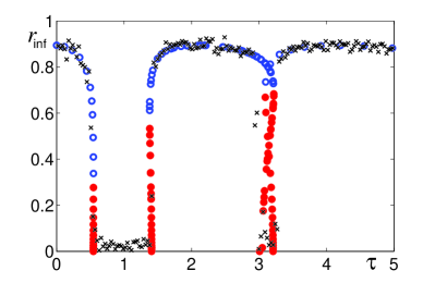
Figure 3: (color online) $\omega_{0}=3$, $\Delta=0.1$, and $k=1$. $r_{\textrm{inf}}$ stands for $|r(\infty)|$. The bifurcation diagram of Eq.(6) is shown. Stable periodic orbits are labeled by blue circles, and unstable periodic orbits, red dots. The order parameters by integrating the Kuramoto model (1) with $N=300$ are marked by black crosses.

a) b)

Figure 4: (color online) $\omega_{0}=3$, $\Delta=0.1$, and $\tau=1$. The bifurcation diagram of Eq.(6) and the period of the bifurcating solutions are shown in a) and b), respectively. $NS$ stands for Neimark-Sacker bifurcation. $SN_{1}$ and $SN_{2}$ are saddle-node bifurcation of periodic orbits. Stable periodic orbits are labeled by blue circles, unstable (1 Floquet exponent with positive real part) periodic orbits, red dots, and unstable (3 Floquet exponents with positive real part) periodic orbits green squares. The order parameters by integrating the Kuramoto model (1) with $N=300$ are marked by black crosses.

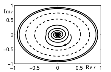
Figure 5: When $k=2.5$ and $\tau=1$, two stable periodic solutions, two unstable periodic solutions (dashed) and a stable equilibrium coexist in Eq.(6).

a) b) c)

Figure 6: When $k=2.5$ and $\tau=1$, system (1) may exhibit incoherence (with initial values uniformly distributed on $[0,2\pi]$), coherence of fast oscillation (with initial values uniformly distributed on $[0,\pi]$), or coherence of slow oscillation (with initial values uniformly distributed on $[0,0.2\pi]$). In the figures, dots stand for the points with $\theta_{j}(t)=2\pi$.

If we fix $\tau=1$ and let $k$ vary, we obtain simulation results in Figure 4(a). By using DDE-Biftool and computing the numbers of Floquet exponents with positive real part, the order parameters, together with two saddle-node points and a Neimark-Sacker bifurcation point, are shown. As $k$ increases, the two branches of bifurcating solutions have nearly the same order parameters, but they can be distinguished by periods. In Figure 4(b) we calculate the periods of the two branches of bifurcating periodic solutions, including the fast and slow oscillations.

In Figure 4(a), one can also find from Figure 2(b) that the simulation results coincide with the theoretical results. Between the saddle-node point and the Hopf bifurcation point, stable incoherent and coherent states coexist, i.e., the hysteresis loop. Particularly, we find an interesting phenomenon near $k=2.5$ (in region I), that is after two times of saddle-node bifurcations, two stable coherent states, two unstable coherent states and a stable incoherent state coexist, i.e., two hysteresis loops intersect. These coexisting solutions of (6) are shown by DDE-Biftool in Figure 5. Recall that (6) is an infinite-dimensional functional differential equation Halefde , thus the unstable periodic orbits do not separate the two stable periodic orbits.

Fixing $\tau=1$ and $k=2.5$, we perform three simulations about Kuramoto model (1) as shown in Figure 6, where we find different initial values lead the Kuramoto model to incoherence and coherence respectively. The two kinds of stable periodic oscillations, shown in Figure 4 and Figure 5 with periods 1.31 and 6.09, are simulated in Figure 6 (b-c).

V.4 Delay-coupled Hindmarsh-Rose neurons

Consider the following coupled Hindmarsh-Rose system HRref ; HRref2

$$\begin{array}[]{l}\dot{x}_{j}=y_{j}-x_{j}^{3}+3x_{j}^{2}-z_{j}+3\\ \dot{y}_{j}=1-5x_{j}^{2}-y_{j}~{}~{}~{}~{}~{}~{}~{}~{}~{}~{}~{}~{}~{}~{}~{}~{}~{}~{}~{}~{}~{}~{}~{}~{}~{}~{}~{}~{}j=1,2,\ldots,N\\ \dot{z}_{j}=0.006[4(x_{j}+I_{j})-z_{j}]+\frac{k}{N}\sum\limits_{i=1}^{N}[z_{i}(t-\tau)-z_{j}]\end{array}$$ (21)

where the random values $I_{j}$ are Gaussian distributed with mean 1.56 and variance 0.5. Thus this is a near-identical, delay-coupled system.

Choosing $N=100$, $k=2$ and $\tau=4$, we perform three groups of simulations as shown in Figure 7. In the figures we find different initial values lead the system to the incoherent state or one of at least two coherent states with different periods as well.

a) b) c)

Figure 7: $k=2$, $\tau=4$ and $t\in[0,50]$. a) When the initial values are uniformly distributed in $[1,4.5]$, system (21) is incoherence. b) When the initial values are uniformly distributed in $[1,2.5]$, system (21) exhibits synchronized states with period near 7. c) When the initial values are uniformly distributed in $[1,1.2]$, system (21) exhibits synchronized states with period near 4.8. In the figures, dots stand for local maxima of $z_{j}(t)$.

VI Conclusion and Discussion

In this paper, we study the delay coupled Kuramoto oscillators on the OA manifold from the point of view of Bautin and double Hopf bifurcation analysis. Complete bifurcation sets are given in Figure 2 and the existence of coherent and incoherent states are listed in Table 1. Through the bifurcation analysis, we find, even in a model as simple as (1), the dynamical behavior is complicated: both theoretical investigations and numerical simulations indicate that Bautin bifurcation and double Hopf bifurcation are very common and must appear in this model, which bring hysteresis loop, multistability and oscillations on torus, respectively. We have theoretically proved that system (6) must undergo Bautin bifurcations thus hysteresis loop always exists in the delay Kuramoto model (1). Particularly, two hysteresis loops may intersect in certain region, which yields that four coherent states (two of which are stable) and a stable incoherence coexist in Kuramoto model. The coexistence of stable coherent and incoherent states are all simulated.

Mathematically, an interesting relation is revealed from Corollary 1: for small $\tau$, Bautin bifurcation value is $k\propto\tau^{-1/2}$ for $\Delta\ll 1$ and $k\propto\Delta$ for $\Delta\gg 1$. In case of Kuramoto model with near identical oscillators, the former applies. Hence we know that the Bautin bifurcation points moves downwards in the $\tau-k$ plane as the increasing of $\tau$.

In the current model, we have theoretically proved that, at all Bautin bifurcation points, one always have Re$l_{2}(0,0)<0$, thus the dynamical behavior near these points are clear as shown in Figure 1. However, near the double Hopf points, the situation is not completely clear, because there are twelve kinds of unfoldings near a double Hopf point homs and we cannot theoretically determine the sign of $b_{0}$, $c_{0}$ $d_{0}$ and $d_{0}-b_{0}c_{0}$ in general. The numerical example in Section 5 is a special and “simple” case of double Hopf bifurcation, but we still find two coexisting synchronized states in the model. Sometimes, stable 2-torus or 3-torus may appear after several times of Neimark-Sacker bifurcations of periodic solutions (e.g., case VIa homs ), which may correspond to rotating waves in the Kuramoto model. Even though such situations are complicated, the normal form (20) can still provide clear bifurcation sets near the double Hopf points.

For practical usage, we simulate a system of delay-coupled Hindmarsh-Rose neurons. We find the results in this paper agree well with a system of delay-coupled Hindmarsh-Rose neurons. In the simulation, we also find two coexisting stable coherent states and one stable incoherent state. It is worth mentioning that there are recently many results about the periodic oscillation or phase synchronization arisen from mathematical biology newnewnew ; nnn1 . Linking the results in the current paper and these biological models will be an interesting work and is left as a future study.

References

- (1) Y. Kuramoto, Self-entrainment of a population of coupled non-linear oscillators, in: H. Arakai (Ed.), International Symposium on Mathematical Problems in Theoretical Physics, Lecture Notes in Physics, (Springer, New York, 1975)
- (2) S.H. Strogatz, Exploring complex networks, Nature 410, 268–276 (2001)
- (3) A. Pikovsky, M. Rosenblum and J. Kurths, Synchronization: A Universal Concept in Nonlinear Sciences, (Cambridge university press, New York, 2003)
- (4) Y. Kuramoto, Chemical Oscillations, Waves, and Turbulence, (Springer, Berlin, 1984)
- (5) A.T. Winfree, Biological rhythms and the behavior of populations of coupled oscillators, J. Theoret. Biol. 16, 15–42 (1967)
- (6) D.C. Michaels, E.P. Matyas and J. Jalife, Mechanisms of sinoatrial pacemaker synchronization: a new hypothesis, Circulation Res. 61, 704–714 (1987)
- (7) C. Liu, D.R. Weaver, S.H. Strogatz and S.M. Reppert, Cellular construction of a circadian clock: period determination in the suprachiasmatic nuclei, Cell 91, 855–860 (1997)
- (8) Z. Jiang and M. McCall, Numerical simulation of a large number of coupled lasers, J. Opt. Soc. Am. 10, 155 (1993)
- (9) S.Yu. Kourtchatov, V.V. Likhanskii, A.P. Napartovich, F.T. Arecchi and A. Lapucci, Theory of phase locking of globally coupled laser arrays, Phys. Rev. A 52, 4089 (1995)
- (10) K. Wiesenfeld, P. Colet and S.H. Strogatz, Frequency locking in Josephson arrays: connection with the Kuramoto model, Phys. Rev. E 57, 1563 (1998)
- (11) M.K.S. Yeung and S.H. Strogatz, Time delay in the Kuramoto model of coupled oscillators, Phys. Rev. Lett. 82, 648 (1999)
- (12) S. Kim, S.H. Park and C.S. Ryu, Multistability in coupled oscillator systems with time delay, Phys. Rev. Lett. 79, 2911 (1997)
- (13) S. Yanchuk and P. Perlikowski, Delay and periodicity, Phys. Rev. E 79, 046221 (2009)
- (14) M.Y. Choi, H.J. Kim, D. Kim and H. Hong, Synchronization in a system of globally coupled oscillators with time delay, Phys. Rev. E 61, 371 (2000)
- (15) E. Ott and T.M. Antonsen, Low dimensional behavior of large systems of globally coupled oscillators, Chaos 18 037113 (2008)
- (16) E. Ott and T.M. Antonsen, Long time evolution of phase oscillator systems, Chaos 19, 023117 (2009)
- (17) W.S. Lee, E. Ott and T.M. Antonsen, Large coupled oscillator systems with heterogeneous interaction delays, Phys. Rev. Lett. 103, 044101 (2009)
- (18) D.V.R. Reddy, A. Sen and G.L. Johnston, Time delay effects on coupled limit cycle oscillators at Hopf bifurcation, Physica D, 129, 15–34 (1999)
- (19) Y. Guo and B. Niu, Amplitude death and spatiotemporal bifurcations in nonlocally delay-coupled oscillators, Nonlinearity 28, 1841–1858 (2015)
- (20) B. Niu and Y. Guo, Bifurcation analysis on the globally coupled Kuramoto oscillators with distributed time delays, Physica D 266, 23–33 (2014)
- (21) S. Guo, Y. Chen and J. Wu, Two-parameter bifurcations in a network of two neurons with multiple delays, J. Differential Equations, 244, 444–486 (2008)
- (22) A.V. Ion and R.M. Georgescu, Bautin bifurcation in a delay differential equation modeling leukemia, Nonl. Anal., TMA, 82, 142–157 (2013)
- (23) B. Zhen and J. Xu, Bautin bifurcation analysis for synchronous solution of a coupled FHN neural system with delay, Commun. Nonlinear Sci. Numer. Simulat. 15, 442–458 (2010)
- (24) D.C. Braga, L.F. Mello, C. Rocşoreanu and M. Sterpu, Control of planar Bautin bifurcation, Nonlinear Dyn. 62, 989–1000 (2010)
- (25) J. Guckenheimer and P. Holmes, Nonlinear Oscillations, Dynamical Systems, and Bifurcations of Vector Fields, (Springer, New York, 1983)
- (26) Y.A., Kuznetsov, Elements of Applied Bifurcation Theory, (Springer, New York, 1998)
- (27) J. Hale and S.M. Verduyn Lunel, Introduction to Functional Differential Equations, (Springer, New York, 1993)
- (28) B. Hassard, N.D. Kazarinoff and Y. Wan, Theory and Applications of Hopf Bifurcation, (Cambridge Univ. Press, Cambridge, 1981)
- (29) T. Faria and L. Magalhães, Normal forms for retarded functional differential equation with parameters and applications to Hopf bifurcation, J. Differential Equations, 122, 181-200 (1995)
- (30) Nayfeh, A.H.: Introduction to Perturbation Techniques, Wiley, New York (1981)
- (31) Yu, P.: Analysis on double Hopf bifurcation using computer algebra with the aid of multiple scales. Nonlinear Dynam. 27, 19–53 (2002)
- (32) Dessi, D., Mastroddi, F., Morino, L.: A fifth-order multiple-scale solution for Hopf bifurcations. Computers and Structures. 82, 2723–2731 (2004)
- (33) Yu, P., Ding, Y., Jiang, W.: Equivalence of the MTS Method and CMR Method for Differential Equations Associated with Semisimple Singularity. International Journal of Bifurcation and Chaos 24, 1450003 (2014)
- (34) Nayfeh, A.H.: Order reduction of retarded nonlinear systems-the method of multiple scales versus center-manifold reduction, Nonlinear Dynam. 51, 483–500 (2008)
- (35) S. Wiggins, Introduction to Applied Nonlinear Dynamical Systems and Chaos, (Springer, New York, 1980)
- (36) K. Engelborghs, T. Luzyanina and G. Samaey, DDE-BIFTOOL v. 2.00: A Matlab package for bifurcation analysis of delay differential equations, (Technical Report TW–330 KU Leuven, Belgium, 2001)
- (37) K. Engelborghs, T. Luzyanina and D. Roose, Numerical bifurcation analysis of delay differential equations using DDE-BIFTOOL, ACM Trans. Math. Software, 28, 1–21 (2002)
- (38) J. L. Hindmarsh and R. M. Rose, A model of neuronal bursting using three coupled first order differential equations, Proc. R. Soc. London, Ser. B 221, 87–102 (1984)
- (39) M. Rosenblum and A. Pikovsky, Delayed feedback control of collective synchrony: an approach to suppression of pathological brain rhythms, Phys. Rev. E 70, 041904 (2004)
- (40) D.A. Vasseur and J.W. Fox, Phase-locking and environmental fluctuations generate synchrony in a predator–prey community, Nature, 460, 1007–1010 (2009)
- (41) A. Colombo, F. Dercole and S. Rinaldi, Remarks on metacommunity synchronization with application to prey‐predator systems, The American naturalist, 171, 430–442 (2008)