Parametrization of the nucleus–nucleus gamma-ray production cross sections below 100 GeV/nucleon: Subthreshold pions and Hard photons

Abstract

“Subthreshold pions” and so-called “hard photons” are two important channels for producing less than 1 GeV $\gamma$-rays and $e^{\pm}$ pairs from nuclear collisions with energy per nucleon below the $\pi$-meson production threshold. I use publicly available experimental data to parametrize these two channels’ $\gamma$-ray and $e^{\pm}$ production cross sections and extend the pion contribution to these particles spectra at higher energies using their corresponding spectra from $pp$ interactions. These parametrizations are valid for collision energy $T_{p}\leq 100$ A GeV and agree reasonably well with the available experimental data. The new parametrizations allow, for the first time, accurate studies of astrophysical $\gamma$-rays below 1 GeV.

I Introduction

Nuclear interactions are ubiquitous in the universe, ranging from thermal plasmas to high energy cosmic rays, being an abundant source of $\gamma$-rays and other secondary particles relevant to astrophysics. At low collision energies and above the Coulomb barrier, inelastic collisions and/or nuclear reactions produce excited nuclei in the final state. De-excitation of these nuclear levels can produce prompt $\gamma$-ray lines as well as a continuum component which is a superposition of many $\gamma$-ray lines with relatively large widths. The main emission lines appear between 0.1 and 10 MeV. At higher collision energies, say $T_{p}\gtrsim 10$ A MeV (MeV/nucleon), nuclear collective modes are excited and produce an additional continuum $\gamma$-radiation component. The most prominent source of this continuum, is the so-called giant dipole resonance which emits most of the $\gamma$-rays between 10 and 25 MeV. The $\gamma$-rays with energy below 25-30 MeV are referred to as the statistical photons and their origin is the nuclear structure.

For nuclear collisions with energy above the $\pi$-meson production threshold ($T_{p}>T_{p\,NN}^{\rm th}\approx 0.28$ A GeV), pions are expected to be produced effectively. Nuclear interactions at such energies produce pions through individual nucleon–nucleon collisions. The decay of these pions produce $\gamma$-rays, $e^{\pm}$ pairs and neutrinos. Similar with $pp$ interactions, the main source of the $\gamma$-rays at high energy nuclear collisions is the decay of the $\pi^{0}$-meson and to a lesser extent the decay of the $\eta$-meson.

These channels however, are not the only ones through which nuclear interactions can produce $\gamma$-rays. Experimental observations show that the continuum radiation from low energy nuclear interactions does not stop with the statistical photons. For photon energies above the giant dipole resonance the $\gamma$-ray spectrum changes its slope and becomes harder. This new direct $\gamma$-ray channel is called the hard photons. Moreover, experimental observations show that nuclear collisions unlike nucleon–nucleon interactions, can produce pions at energies $T_{p}<T_{p\,NN}^{\rm th}$. These pions are called the subthreshold pions and are observed for collision energies as low as 20 A MeV Grimm and Grosse (1985); Grosse (1986). From energetics point of view, the hard photons and subthreshold pions require a mechanism that will extract the energy from many nucleons inside the nucleus. They are partly explained by the Fermi motion, however, the detailed physics related to the cooperative effects is not yet well understood.

Experimental observations have played a crucial role in singling out the main processes responsible for the production of hard photons and subthreshold pions. For instance, the center of mass frame observations show that hard photons have a dipole angular distribution and their production source velocity is close to the nucleon–nucleon velocity in this frame. These suggest that the source of hard photons is the neutron–proton ($np$) bremsstrahlung that occurs during the early stage of the nuclear interaction (see e.g. Nifenecker and Pinston, 1989; Cassing et al., 1990; Schutz et al., 1997). The $pp$ bremsstrahlung has a quadrupole nature, therefore, gives a minor contribution compared to the $np$. Moreover, it is observed that hard photon energy distribution is an exponential function of the form $\sim\exp(-E_{\gamma}/E_{0}^{\gamma})$, with an inverse slope parameter $E_{0}^{\gamma}$ that is experimentally determined. In heavy ion experiments an additional component of direct hard photons is observed, called the thermal hard photons (see e.g. D’Enterria and Martínez, 2000; D’Enterria et al., 2001). This component however, is not important for light nuclei that are relevant in astrophysics.

Subthreshold pions are also produced during the first stage of the nucleus–nucleus collision. In contrast to the hard photons, pion’s mean free path in the nuclear matter is short. As a result, they are reabsorbed and re-emitted several times which leads to their thermalization with the nuclear matter. Therefore, pions energy distribution carries important information about the fireball that is formed in the intermediate phase of the nuclear reaction. Experiments show that the pion energy distribution can be fitted with a Maxwellian distribution. At energies $T_{p}\approx 1$ A GeV, $\Delta$-resonance production becomes significant. Its decay results in the formation of a high energy tail on top of the Maxwellian distribution. At such energies, the experimental data are fitted with more than one Maxwellian distribution (see e.g. Stock, 1986; Cassing et al., 1990; Senger and Ströbele, 1999; Bonasera et al., 2006).

Although for $T_{p}\lesssim T_{p\,NN}^{\rm th}$ interactions there is no theory that can accurately predict the hard photon and subthreshold pion production cross sections, at higher energies however, one can use Glauber’s multiple scattering theory (Glauber, 1955; Franco and Glauber, 1966; Glauber and Matthiae, 1970) as applied in some superposition model (e.g. the wounded-nucleon model (Białłas et al., 1976) or the additive quark model (see e.g. Bialas et al., 1977; Anisovich et al., 1978; Nikolaev, 1981)) to calculate the secondary particle production average and dispersion multiplicity distributions. In these models, the hadron–nucleus and nucleus–nucleus collision are treated as a sequence of nucleon–nucleon or quark(s)–nucleon scatterings. As a result, the average secondary particle production multiplicity of a nucleus–nucleus collision is proportional with the average yield produced by nucleon–nucleon or quark(s)–nucleon interactions. The proportionality factor is called the number of wounded constituents. The so-called nuclear enhancement factor (see e.g. Gaisser and Schaefer, 1992), is an application of the wounded nucleon model in astrophysics. This quantity sums the contributions of all nucleus–nucleus interactions which scale the secondary particle production spectrum produced by $pp$ collisions.

By combining subthreshold pions at low energies with high energy pion production calculations, it is possible to compute pion production cross sections for a wide energy range which can be important in astrophysics. The hard photon and subthreshold pion channels allow nuclear interactions to produce $\gamma$-rays and $e^{\pm}$ pairs at low energies for which the $pp$ interactions do not. Moreover, the $\gamma$-rays from these two channels, significantly contribute in the $\gamma$-ray spectrum below the $\pi^{0}$-bump that is produced by $pp$ interactions. These channels should be taken into account in the identification of the radiation process and the parent particles that produce the $\gamma$-rays (leptonic versus hadronic). This identification should be based on the shape of the measured $\gamma$-ray spectrum below 1 GeV. Surprisingly, so far this question has not been studied even on a qualitative level despite the recent numerous claims of detection of hadronic $\gamma$-rays based on the observations by Fermi-LAT.

In this paper I intend to fill the gap of studies in this area. Although the physics of complex processes of nucleus–nucleus interactions at low energies is not yet fully understood and described by an adequate theory, the available experimental measurements are quite comprehensive to conduct a detailed quantitative study of this important issue. Note that the units used throughout this article are the natural units (i.e. $\hbar=c=k_{B}=1$).

II Hard photons production cross sections

The experimentally supported assertion that the direct photons with energy $E_{\gamma}>30$ MeV are produced through incoherent neutron–proton ($np$) bremsstrahlung is further supported by the fact that their production cross section scales with the number of first $np$ collisions. Following Bertholet et al. (1987), the hard photons production cross section can be parametrized as follows:

$$\sigma_{\gamma}=\sigma_{R}\,\left\langle N_{np}\right\rangle_{b}\,P_{\gamma},$$ (1)

where $\sigma_{R}$ is the reaction cross section, $\left\langle N_{np}\right\rangle_{b}$ is the total number of initial $np$ collisions averaged over the impact parameter and $P_{\gamma}$ is the $\gamma$-ray emission probability in a single collision. We use the parametrization of $\sigma_{R}$ from Cassing et al. (1990) which has the form:

$$\sigma_{R}=10\pi\,r_{0}^{2}\left(A_{p}^{1/3}+A_{t}^{1/3}+b\right)^{2}\!\left(1-\frac{V_{c}}{A_{p}\,T_{p}}\right)~{}\![{\rm mb}].$$ (2)

Here, $r_{0}=1.16$ fm, $b=2.0$ and $T_{p}$ is the projectile kinetic energy per nucleon in the laboratory frame. $V_{c}=1.44\,Z_{p}Z_{t}/R$ is the Coulomb potential of the colliding nuclei in MeV units and $R=1.2\,(A_{p}^{1/3}+A_{t}^{1/3})$ fm. $Z_{p}$, $A_{p}$ and $Z_{t}$ and $A_{t}$ are the charge and mass numbers for the projectile and target nuclei, respectively. The parameter $\left\langle N_{np}\right\rangle_{b}$ is given by:

$$\left\langle N_{np}\right\rangle_{b}=\left\langle A_{F}\right\rangle\,\frac{Z_{p}\,N_{t}+Z_{t}\,N_{p}}{A_{p}\,A_{t}},$$ (3)

where $N_{p}$ and $N_{t}$ are the number of neutrons for the projectile and target, respectively. $\left\langle A_{F}\right\rangle$ is the number of nucleon-nucleon collisions which is given by:

$$\left\langle A_{F}\right\rangle=A_{p}\times\frac{5\,A_{t}^{2/3}-A_{p}^{2/3}}{5\left(A_{p}^{1/3}+A_{t}^{1/3}\right)^{2}},$$ (4)

and it is valid for $A_{p}\leq A_{t}$ Nifenecker and Bondorf (1985).

Using experimental data for the hard photon production cross section $\sigma_{\gamma}$ for $E_{\gamma}>E_{\gamma}^{\rm min}=30$ MeV, Cassing et al. (1990) has parametrized the $\gamma$-ray emission probability $P_{\gamma}$ as:

$$P_{\gamma}=M_{0}\times\exp\left(-\frac{E_{\gamma}^{\rm min}}{E_{0}^{\gamma}}\right),$$ (5)

where, $M_{0}=(5.5\pm 0.1)\times 10^{-4}$ is a constant that is derived from fitting the cross section data; whereas, $E_{0}^{\gamma}$ is found from fitting the hard photon energy distribution spectrum, which has an exponential shape $d\sigma/dE_{\gamma}\sim\exp(-E_{\gamma}/E_{0}^{\gamma})$. If we normalize this function such that its integral from $E_{\gamma}^{\rm min}$ to infinity gives $\sigma_{\gamma}$, the hard photon differential cross section becomes:

$$\frac{d\sigma_{\gamma}}{dE_{\gamma}}=\frac{\sigma_{\gamma}}{E_{0}^{\gamma}}\times\exp\left(\frac{E_{\gamma}^{\rm min}-E_{\gamma}}{E_{0}^{\gamma}}\right).$$ (6)

The hard photon inverse slope parameter $E_{0}^{\gamma}$ is the only missing element in Eqs. (5) and (6). Experimental data show that $E_{0}^{\gamma}$ systematically increases with the collision energy and the available data show two different trends for heavy and for light ions interactions. I have compiled here publicly available experimental data on $E_{0}^{\gamma}$ that are found in the literature and they are recorded in Table 1. These data include a variety of colliding systems for a broad collision energy range. I have parametrized these data in two branches: Data for light projectiles $p$, $\alpha$ (⁴He) and Li, and data for heavier projectiles. These two groups seem to form two distinct clusters and $E_{0}^{\gamma}$ for projectiles heavier than Li is larger than for lighter projectiles. This difference might be related to the absence of Fermi motion of nucleons inside the light nuclei which leads to lesser energetic $np$ collisions, thus to a softer spectrum of $\gamma$-rays. The parametrization of the inverse slope parameter has the form:

$$E_{0}^{\gamma}=a\,\epsilon_{p}^{b},$$ (7)

where $\epsilon_{p}=(T_{p}-V_{c}/A_{p})/m_{p}$ is a dimensionless variable, and $m_{p}$ is the nucleon rest mass which is considered equal to the proton mass. By fitting the experimental data, I find that for light projectiles ($p$, $\alpha$ and Li) $a=60\pm 10$ MeV and $b=0.54\pm 0.06$ and for heavier projectiles $a=182\pm 1$ MeV and $b=0.805\pm 0.002$. Figure 1 compares the experimental data with the parametrization described here as well as with the parametrizations described in (Cassing et al., 1990; Schutz et al., 1997). The figure shows that all parametrizations agree with each other and fit reasonably well the available experimental data.

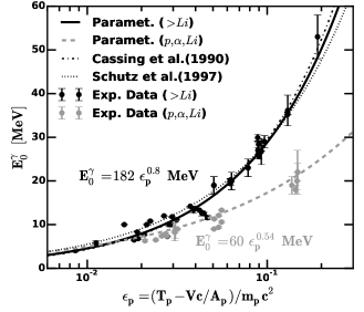
Figure 1: Hard photon inverse slope parameter $E_{0}^{\gamma}$ for $E_{\gamma}>30$ MeV as a function of $\epsilon_{p}=\left(T_{p}-V_{c}/A_{p}\right)/m_{p}$, where, $T_{p}$ is the projectile kinetic energy per nucleon, $V_{c}$ is the Coulomb energy, $A_{p}$ the projectile mass number and $m_{p}$ is the nucleon mass in units of energy. The experimental data that are used here are listed in Table 1. Data in grey color correspond to light projectiles $p$, $\alpha$ and Li, whereas, data in black color belongs to heavier projectiles. The grey thick-dash-line shows the Eq. (7) parametrization for projectiles $p$, $\alpha$ and Li which is $E_{0}^{\gamma}=(60\pm 10)\,\epsilon_{p}^{0.54\pm 0.06}$ MeV; whereas, the black thick-line shows the parametrization for projectiles heavier than Li $E_{0}^{\gamma}=(182\pm 1)\,\epsilon_{p}^{0.805\pm 0.002}$ MeV. The thin dash-dot line is the parametrization given in Cassing et al. (1990) and the dots curve is the parametrization given in Schutz et al. (1997).

Figure 2 compares the $P_{\gamma}$ emission probability parametrization in Eq. (5) using $E_{0}^{\gamma}$ from Eq. (7), against the experimental data compiled in Cassing et al. (1990). The parametrizations used in Cassing et al. (1990) and Schutz et al. (1997) are also included and, they differ only on the parametrization of $E_{0}^{\gamma}$. All these parametrizations agree reasonably well with each other and with the available experimental data.

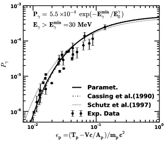
Figure 2: Hard photon emission probability $P_{\gamma}$ for $E_{\gamma}>E_{\gamma}^{\rm min}=30$ MeV as a function of $\epsilon_{p}$. The experimental data points are compiled by Cassing et al. (1990). The black line is the parametrization shown in Eqs. (5) and (7). The thin dash-dot line and the dotted line are the parametrizations given in Cassing et al. (1990) and Schutz et al. (1997), respectively.

If we include Eq. (1) and Eq. (5) in Eq. (6), the hard photons differential cross section for $E_{\gamma}>E_{\gamma}^{\rm min}=30$ MeV is further simplified:

$$\frac{d\sigma_{\gamma}}{dE_{\gamma}}=\frac{\sigma_{R}\,\left\langle N_{np}\right\rangle_{b}\,M_{0}}{E_{0}^{\gamma}}\times\exp\left(-\frac{E_{\gamma}}{E_{0}^{\gamma}}\right).$$ (8)

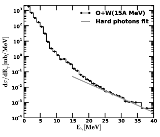
Figure 3: Gamma-ray production differential cross section for ¹⁶O + ¹⁸⁴W intereactions at $T_{p}=15$ A MeV Breitbach et al. (1989). The thick gray line is the hard photon fit using the parametrization in Eq. (8).

To conclude, Fig. 3 shows a typical $\gamma$-ray spectrum that includes both the statistical and hard photons produced by ¹⁶O + ¹⁸⁴W interactions at $T_{p}=15$ A MeV Breitbach et al. (1989). We see that the low energy statistical photons have larger cross sections compared to hard photons for $E_{\gamma}>30$ MeV. By increasing the collision energy the hard photon spectra becomes larger and harder. Hard photons dominate the $\gamma$-ray continuum for collision energies below $T_{p}<100$ A MeV. Above this energy the $\pi^{0}$-meson production start to dominate.

Table 1: References for the hard photon inverse slope parameter $E_{0}^{\gamma}$ experimental data.

System	$T_{p}$ [A MeV]	Reference
C+Mo	11	Gossett et al. (1990)
O+W	15	Breitbach et al. (1989)
N+(C,Zn,Pb)	20–40	Stevenson et al. (1986)
Kr+Ni;Ta+Au	29.5–60	Martínez et al. (1995)
Pb+Au	29.5–60	Martínez et al. (1995)
He+(C,Zn,Pb)	25,53	Tam et al. (1988)
Li+(Li,Pb);Ne+Mg	30	Tam et al. (1989)
Ar+(Ca,Pb)	30	Tam et al. (1989)
Ar+Au	30	Njock et al. (1986)
Ar+Gd	44	Hingmann et al. (1987)
Kr+(C,Ag)	44	Bertholet et al. (1987)
(Pb,Ta)+Au;Kr+Ni	30–60	Schutz et al. (1997)
C+C	48–84	Grosse et al. (1986)
D+(C,Zn,Pb)	53	Tam et al. (1988)
Kr+Ni	60	Martínez et al. (1994)
Ar+(C,Al,Cu)	85	Njock et al. (1988)
Xe+Sn	89,124	Clayton et al. (1989)
Ar+(C,Au)	95	Schubert et al. (1994)
p+(C,O,Al,Cu,Pb)	140	Edgington and Rose (1966)
Ar+Ca	180	Martínez et al. (1999)

III Subthreshold pion production

III.1 Total production cross section $\sigma_{\pi}$

The pion production cross section from nuclear collisions is well studied for a wide range of collision energies and for a variety of colliding nuclei. If pions in nucleus–nucleus ($A+B$) interactions are indeed produced through individual in-medium nucleon–nucleon ($N+N$) collisions, then their production cross sections or multiplicities should scale with the number of participating nucleons. Unlike the free nucleon–nucleon collisions the in-medium ones are enhanced by the Fermi motion of nucleons in the interactions zone. A common parametrization of the meson production cross section in $A+B$ collisions is (see e.g. Metag, 1993):

$$\sigma_{\pi}=\sigma_{R}\,\left\langle A_{part}\right\rangle_{b}\,P_{\pi},$$ (9)

where $\sigma_{R}$ is the $A+B$ reaction cross section given in Eq. (2), $P_{\pi}$ is the in-medium pion production probability per participant and $\left\langle A_{part}\right\rangle_{b}$ is the number of participants calculated within the geometrical model and averaged over the impact parameter $b$ (see e.g. Hüfner and Knoll, 1977; Cugnon et al., 1981):

$$\left\langle A_{part}\right\rangle_{b}=\frac{A_{p}\,A_{t}^{2/3}+A_{t}\,A_{p}^{2/3}}{\left(A_{p}^{1/3}+A_{t}^{1/3}\right)^{2}}.$$ (10)

I have collected public available experimental pion production cross section data that cover the nuclear collision energy range $20~{}{\rm A~{}MeV}<T_{p}<100~{}{\rm A~{}GeV}$ and for nuclei that are lighter than Zr. These data are recorded in Table 2–4. Using Eq. (9) and these cross section data, one can compute the probability $P_{\pi}$, which is plotted in Fig. 4 as a function of $\epsilon_{p}=(T_{p}-V_{c}/A_{p})/m_{p}$.

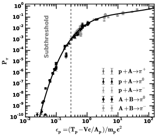
Figure 4: The universal pion production probability as a function of $\epsilon_{p}$. All experimental data shown here are listed in Table 2–4. The fitting curve is the parametrization given in Eq. (11), $P_{\pi}/(\mathcal{I}_{\pi}\times\zeta)=\epsilon_{p}^{-1/4}\times\exp\left[\epsilon_{p}^{-1/4}\left(0.0057\,x^{4}+0.019\,x^{3}-0.19\,x^{2}+1.07\,x-3.7\right)\right]$ where $x=\log(\epsilon_{p})$.

It is clear from Fig. 4 that the experimental $P_{\pi}$ data show a systematic increase with the collision energy per nucleon. I have parametrized the probability $P_{\pi}$ for $T_{p}\leq 100$ A GeV as follows:

$$\begin{split}\Pi_{4}(x)&=a_{0}+a_{1}\,x+a_{2}\,x^{2}+a_{3}\,x^{3}+a_{4}\,x^{4}\\ P_{\pi}&=\epsilon_{p}^{-1/4}\times\exp\left[\epsilon_{p}^{-1/4}\times\Pi_{4}(x)\right]\times\mathcal{I}_{\pi}\times\zeta,\end{split}$$ (11)

where $x=\log(\epsilon_{p})$. After fitting the experimental data one finds that $a_{0}=-(3.70\pm 0.05)$, $a_{1}=1.07\pm 0.06$, $a_{2}=-(0.19\pm 0.03)$, $a_{3}=(19\pm 7)\times 10^{-3}$ and $a_{4}=(5.7\pm 1.8)\times 10^{-3}$.

Different nuclear interactions produce different $\pi^{+}$, $\pi^{0}$ and $\pi^{-}$ yields. The function $\mathcal{I}_{\pi}$ takes into account these differences for a particular $A+B$ interaction by assuming that the differences arise due to isospin symmetry. Function $\mathcal{I}_{\pi}$ normalizes the probability $P_{\pi}$ for one of the $\pi$-mesons with respect to the $\pi^{0}$ one. Therefore, by adopting the isospin relations that exist between the three different pion yields from nucleon–nucleon interactions (see e.g. Golokhvastov, 2001), one finds:

$$\mathcal{I}_{\pi}(\xi_{p},\xi_{t})=\begin{cases}(3+\xi_{p}+\xi_{t})/4&\text{for }\pi^{+}\\ 1&\text{for }\pi^{0}\\ (5-\xi_{p}-\xi_{t})/4&\text{for }\pi^{-}\\ \end{cases}$$ (12)

where $\xi_{p}=Z_{p}/A_{p}$ and $\xi_{t}=Z_{t}/A_{t}$ give the ratio between the number of protons and the total number of nucleons for the projectile and target nuclei, respectively. Function $\zeta(T_{p},A_{p},A_{t})$, on the other hand, ensures that pion production cross section for a given nucleus–nucleus interaction approaches zero when the collision energy approaches the absolute kinematic threshold, the kinetic energy per nucleon of which is given by:

$$T_{p}^{\rm th}=\left(\frac{1}{A_{p}}+\frac{1}{A_{t}}\right)m_{\pi}+\frac{m_{\pi}^{2}}{2m_{p}\,A_{p}A_{t}},$$ (13)

where $m_{\pi}$ is the pion mass. Based on the available experimental data near the kinematic threshold, a reasonably good approximation of $\zeta$ function is:

$$\zeta=\tanh\left(\max\left[0\,;\;1-\left(\frac{T_{p}^{\rm th}}{T_{p}}\right)^{3}\right]\right)^{1/4},$$ (14)

The function $\max$ makes $\zeta$ and $P_{\pi}$ equal zero for $T_{p}\leq T_{p}^{\rm th}$. The function $\zeta$ does not effect the shape of $P_{\pi}$ except near the pion absolute kinematic threshold.

The universal $P_{\pi}$ function that is plotted in Fig. 4 is actually the $P_{\pi}/(\mathcal{I}_{\pi}\times\zeta)$ as was defined in Eq. (11).

III.2 Differential cross section $d\sigma_{\pi}/dE_{\pi}$

Experimental observations for $T_{p}\lesssim 1$ A GeV nuclear collisions show that the pion energy distribution has an exponential shape at high energies and it peaks at low energies at several tens of MeV. For head-on nucleus–nucleus collisions, the pion spectrum to a good approximation is isotropic; therefore, a statistical model is widely used to fit the experimental data (see e.g. Stock, 1986; Senger and Ströbele, 1999). I assume here that the pion energy distribution for $T_{p}<1$ A GeV is given by a single relativistic Maxwell–Jüttner distribution $f_{MB}(E_{\pi},T_{0})$, therefore, the pion differential cross section is:

$$\frac{d\sigma_{\pi}}{dE_{\pi}}=\frac{\sigma_{\pi}}{m_{\pi}}\times f_{MB}(E_{\pi},T_{0}).$$ (15)

Where, $E_{\pi}$ is the pion total energy and $T_{0}$ is the pion temperature. Experiments show that the pion temperature increases systematically with the collision energy and they show that $T_{0}$ is almost independent on the pion species or the initial colliding nuclei. I have compiled here publicly available experimental pion temperature data for projectile energies below few GeV/nucleon and they are listed in Table 5. For collision energies below 4 A GeV, the following formula can parametrize reasonably well the pion temperature data:

$$T_{0}=(57\pm 8)\,\epsilon_{p}^{1/2}+(2.4\pm 1.2)~{}{\rm MeV}.$$ (16)

Figure 5 compares this parametrization with the available experimental data.

Note that the $\Delta$-resonance start to be produced effectively at several hundreds of MeV per nucleon and it becomes non-negligible for collision energies around 1 A GeV or higher. Its decays produce high energy pions that modify the tail of the Maxwellian distribution; therefore, Eq. (15) may not be a good representation of the high energy pions and their decaying products near the kinematic limit.

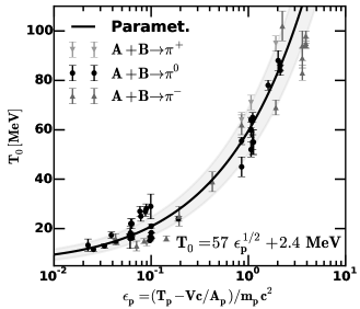
Figure 5: The pion temperature as a function of $\epsilon_{p}$. The experimenal data points are listed in Table 5. The line represents the parametrization given in Eq. (16) and the shaded area is the $1\sigma$ fitting bounds.

Table 2: References to $p+A\to\pi^{0}$ experimental cross section data.

System	$T_{p}$ [MeV]	Reference
p+(C,Al,Ni)	201	Bellini et al. (1989)
p+C	470	Bayukov et al. (1957)
p+D	660	Bayukov et al. (1957)
p+(Li,C,O,Al,Cu)	665	Dunaitsev and Prokoshkin (1964)
p+He	380–970	Pollack and Fazio (1963)

Table 3: References to $A+B\to\pi^{0}$ experimental cross section data.

System	$T_{p}$ [A MeV]	Reference
(He,O)+Mg	24–43	Waters et al. (1993)
N+Al	35	Braun-Munzinger et al. (1984)
O+Al	38	Julien et al. (1988)
Ar+Ca	44	Heckwolf et al. (1984)
C+(C,Ni)	60–84	Noll et al. (1984)
O+Al	94	Badalá et al. (1993)
Ar+(Al,Ni)	95	Badalà et al. (1996)
O+(Al,Ni)	95	Moisan et al. (1992)
Ar+Ca	180	Martínez et al. (1999)
Ar+Ca	1000	Schwalb et al. (1994)
(D,He,Ca)+Ca	1040,1060	Holzmann et al. (1997)
C+C	1040,1060	Holzmann et al. (1997)
C+C	800–2000	Averbeck et al. (2003)
C+C	1000,1800	Laue et al. (2000)

Table 4: References to charged pion production experimental cross section and multiplicity data.

System	$T_{p}$ [A MeV]	Reference
$\pi^{+}$
p+Ni	201	Badala et al. (1992)
p+He	380–970	Pollack and Fazio (1963)
p+(D,C,O,
Al,Ni,Cu)	585	Crawford et al. (1980)
p+(Be,Al)	13.7 $\times 10^{3}$	Abbott et al. (1992)
p+Mg	99.1 $\times 10^{3}$	Whitmore et al. (1994)
$\pi^{-}$
p+He	380–970	Pollack and Fazio (1963)
p+(D,Be,C,O)	585	Crawford et al. (1980)
p+(Al,Ni,Cu)	585	Crawford et al. (1980)
p+C	3.4$\times 10^{3}$	Agakishiyev et al. (1985)
C+(C,Ne,Si)	3.7$\times 10^{3}$	Aksinenko et al. (1980)
C+(Cu,Zr)	3.7$\times 10^{3}$	Aksinenko et al. (1980)
p+C	9.1$\times 10^{3}$	Baatar et al. (1980)
p+C	9.1$\times 10^{3}$	Armutliisky et al. (1988)
p+(Be,Al)	13.7 $\times 10^{3}$	Abbott et al. (1992)
p+Ne	27.1 $\times 10^{3}$	Miller and Nowak (1975)
p+Mg	99.1 $\times 10^{3}$	Whitmore et al. (1994)
p+Mg	199.1 $\times 10^{3}$	Brick et al. (1989)
(D,He,C)+C	3.37$\times 10^{3}$	Agakishiyev et al. (1985)

Table 5: References to the experimental $\pi$-mesons temperature data.

System	$T_{p}$ [A MeV]	Reference
$\pi^{+}$
C+C	85	Johansson et al. (1982)
Ni+Ni	800–1800	Müntz et al. (1997)
$\pi^{0}$
O+(Al,Ni)	25	Young et al. (1986)
Ar+(C,Al,Ni,Ag,Au),
Au+Au	25–95	Piasecki et al. (2010)
Xe+Au	44	Mayer et al. (1993)
Kr+Ni;Ta+Au	60	Schutz et al. (1997)
C+(C,Ni)	60–84	Noll et al. (1984)
O+Al	94	Badalá et al. (1993)
O+Al	95	Moisan et al. (1992)
Ar+Ca	180	Martínez et al. (1999)
Ar+Ca	800	Marín et al. (1997)
Ar+Ca;Kr+Zr;Au+Au	1000	Schwalb et al. (1994)
(Ca,Ar)+Ca	800–2000	Averbeck et al. (2003)
C+C;Ni+Ni	800–2000	Averbeck et al. (2003)
(D,He,Ca)+Ca;C+C	1040–1060	Holzmann et al. (1997)
$\pi^{-}$
C+N	41–135	Suzuki et al. (1991)
Ar+KCl	1800	Brockmann et al. (1984)
C+Al	183–2100	Nagamiya et al. (1982)
(D,He,C)+C	3.37$\times 10^{3}$	Backović et al. (1992)
He+(Li,C);C+Ca	3.66$\times 10^{3}$	Chkhaidze et al. (1992)

IV Gamma-rays and $e^{\pm}$ spectra

Employing the kinematics of the pion decay and the pion differential cross section defined in Eq. (15) one can now calculate the $\gamma$-ray and $e^{\pm}$ pair production spectra for $T_{p}<1$ A GeV.

At higher energies, nuclear matter effects are expected to weaken; therefore, the pion production spectrum from nucleus–nucleus and nucleon–nucleon collisions are expected to be similar in shape. Recent high energy experiments find that the pion spectrum produced by $p+A$ and $A+B$ interactions in the forward hemisphere are similar to $pp$. Deviations from $pp$ are observed in the backward hemisphere where an excess of low energy pions are produced. A recent comprehensive study of the pion spectrum produced by $pp$ and $p+$C at 158 GeV/c show that the deviations between a two-component model – that is constructed from the $pp$ data – and the $p+$C pion data are less than 30–40 % (Barr et al., 2007). In another study, a comparison of the experimental pion transverse mass distribution spectra below 1 GeV show that the deviations of Be+Be and Pb+Pb from $pp$ interactions with $T_{p}<100$ A GeV is less than 20 % and 40 %, respectively (see e.g. Andronov and for the NA61/SHINE Collaboration, 2015). Combining these experimental findings, one may conclude that the expected deviations for the pion energy distribution shape between $pp$ and the light nuclear interactions that are relevant in astrophysics should not be larger than 30–40 % for collisions with $T_{p}\leq 100$ A GeV. Thus, for simplicity I assume here that nucleus–nucleus and nucleon–nucleon collisions with $1\leq T_{p}\leq 100$ A GeV have identical pion spectral shape. As a result, the secondary particle production spectra for nucleus–nucleus collisions are calculated using their $pp$ spectra for which accurate parametrizations already exist (see e.g. Kamae et al., 2006; Kafexhiu et al., 2014).

IV.1 $\gamma$-ray differential cross section $d\sigma_{\gamma}/dE_{\gamma}$

The main channels through which nucleus–nucleus interactions produce $\gamma$-rays with energy $E_{\gamma}>30$ MeV are the hard photons, $A+B\to\gamma$ and the neutral pion decay, $A+B\to\pi^{0}\to 2\gamma$. While the energy distribution of directly produced hard photons for a fixed projectile energy is described by Eq. (8), the distribution of $\pi^{0}\to 2\gamma$ decay is determined by the $d\sigma_{\pi}/dE_{\pi}$ of the intermediate $\pi^{0}$-mesons given in Eq. (15) and by the kinematics of their decay:

$$\frac{d\sigma_{\gamma}}{dE_{\gamma}}=2\times\int\limits_{Y_{\gamma}}^{E_{\pi}^{\rm max}}\frac{d\sigma_{\pi}}{dE_{\pi}}\,\frac{dE_{\pi}}{P_{\pi}}.$$ (17)

Here, the quantity $Y_{\gamma}$ is:

$$Y_{\gamma}=E_{\gamma}+\frac{m_{\pi}^{2}}{4\,E_{\gamma}}~{},$$ (18)

and $E_{\pi}^{\rm max}$ is the maximum $\pi^{0}$ energy in the laboratory frame which is given by:

$$\begin{split}E_{\pi}^{\rm max}&=\gamma_{CM}\,(E_{\pi}^{CM}+P_{\pi}^{CM}\,\beta_{CM})\\ \gamma_{CM}&=\frac{A_{p}\,T_{p}+M_{A}+M_{B}}{\sqrt{s}}\\ s~{}~{}~{}&=\left(M_{A}+M_{B}\right)^{2}+2\,M_{B}\left(A_{p}\,T_{p}+M_{A}\right)\\ E_{\pi}^{CM}&=\frac{s-\left(M_{A}+M_{B}\right)^{2}+m_{\pi}^{2}}{2\sqrt{s}}.\\ \end{split}$$ (19)

Where, $T_{p}$ is the projectile kinetic energy per nucleon, $s$ is the center of mass energy squared. $\beta_{CM}$, $\gamma_{CM}$ and $E_{\pi}^{CM}$ and $P_{\pi}^{CM}$ are the center of mass velocity, Lorentz factor and pion maximum energy and momentum, respectively. $M_{A}$ and $M_{B}$ are the mass of the projectile $A$ and the target $B$, respectively.

By performing the integration of Eq. (17), one finds:

$$\begin{split}\frac{d\sigma_{\gamma}}{dE_{\gamma}}=&\frac{2\,\theta_{\pi}\,\sigma_{\pi}}{m_{\pi}\,K_{2}(\theta_{\pi}^{-1})}\left[\left(1+\frac{Y_{\gamma}}{T_{0}}\right)\times\exp\left(-\frac{Y_{\gamma}}{T_{0}}\right)-\right.\\ &\qquad\qquad\left.\left(1+\frac{E_{\pi}^{\rm max}}{T_{0}}\right)\times\exp\left(-\frac{E_{\pi}^{\rm max}}{T_{0}}\right)\right].\end{split}$$ (20)

The pion temperature $T_{0}$ is given in Eq. (16), $\theta_{\pi}=T_{0}/m_{\pi}$, $\sigma_{\pi}$ is the $\pi^{0}$ production cross section see Eq. (9), $Y_{\gamma}$ varies between $m_{\pi}\leq Y_{\gamma}\leq E_{\pi}^{\rm max}$ and $K_{2}(x)$ is the modified Bessel function of the second kind.

For collision energies $T_{p}\geq 1$ A GeV, the $\pi^{0}$ energy distribution for $A+B$ and nucleon–nucleon collisions are equal $f_{AB}^{\pi^{0}}=f_{NN}^{\pi^{0}}$. By averaging the pion spectrum over different nucleon–nucleon collisions (i.e. $pp$, $np$ and $nn$), it is shown in the Appendix A that $f_{AB}^{\pi^{0}}=f_{pp}^{\pi^{0}}$. Therefore, their respective $\pi^{0}\to 2\gamma$ energy distributions should be equal $f_{AB}^{\gamma}=f_{pp}^{\gamma}$. To calculate $f_{pp}^{\gamma}$, the recent parametrization of the $pp\to\pi^{0}\to 2\gamma$ production cross sections is adopted Kafexhiu et al. (2014). Using the $\gamma$-ray production differential cross section $d\sigma^{\gamma}_{pp}/dE_{\gamma}$ and the pion production cross section $\sigma^{\pi}_{pp}$, the $\gamma$-ray energy distribution function is given by $f_{pp}^{\gamma}=(\sigma^{\pi}_{pp})^{-1}\times d\sigma^{\gamma}_{pp}/dE_{\gamma}$. As a result, the nucleus–nucleus $\gamma$-ray production differential cross section is given by $d\sigma^{\gamma}_{AB}/dE_{\gamma}=\sigma^{\pi}_{AB}\times f_{pp}^{\gamma}$, where, $\sigma^{\pi}_{AB}$ is calculated using Eq. (9).

IV.2 $e^{\pm}$ pair production spectra

After production, charged pions quickly decay into muons which are unstable and further decay into electrons and positrons, $\pi^{\pm}\to\mu^{\pm}\to e^{\pm}$. Although, electrons and positrons cannot be detected directly from an astrophysical source, they however, can emit $\gamma$-rays through radiative processes such as e.g. bremsstrahlung and synchrotron radiation.

The decay kinematics of charged pions into $e^{\pm}$ is more complex than $\pi^{0}\to 2\gamma$ because it involves the muon spin and the three body decay kinematics. A useful quantity that is found in the literature, is the $e^{\pm}$ energy distribution for a fixed pion energy (see e.g. Scanlon and Milford, 1965; Dermer, 1986). This quantity is convolved with the pion spectrum to obtain the $e^{\pm}$ production spectra.

The charged pion energy distribution for $A+B$ collisions for $T_{p}<1$ A GeV is described by Eq. (15). Assuming that the projectile $A$ flux is given by $J_{A}(T_{p})$ and the target number density is $n_{B}$, we can calculate the pion production spectrum:

$$\frac{dN_{\pi}}{dE_{\pi}}=4\pi\,n_{B}\int\limits_{T_{p}^{\rm th}}^{\infty}dT_{p}\;J_{A}(T_{p})\;\frac{d\sigma_{\pi}^{AB}}{dE_{\pi}}(T_{p},E_{\pi}).$$ (21)

By convolving this quantity with the $e^{\pm}$ normalized energy distribution for a single pion energy $\Phi(\gamma_{\pi},E_{e})$ Dermer (1986), one can calculate the $e^{\pm}$ emissivity as follows:

$$\frac{dN}{dE_{e}}=\int\limits_{\bar{\gamma}_{\pi}}^{\infty}d\gamma_{\pi}\;\frac{dN_{\pi}}{d\gamma_{\pi}}(\gamma_{\pi})\times\Phi(\gamma_{\pi},E_{e}).$$ (22)

Where, $\gamma_{\pi}=E_{\pi}/m_{\pi}$, $\bar{\gamma}_{\pi}=1$ if $E_{e}<E_{e}^{\rm max}$ and $\bar{\gamma}_{\pi}=\frac{1}{2}(E_{e}/E_{e}^{\rm max}+E_{e}^{\rm max}/E_{e})$ if $E_{e}>E_{e}^{\rm max}$. $E_{e}^{\rm max}=m_{\mu}\gamma_{\mu}(1+\beta_{\mu})/2$, $\gamma_{\mu}=(m_{\pi}^{2}+m_{\mu}^{2})/2m_{\pi}m_{\mu}$, $\beta_{\mu}=(1-\gamma_{\mu}^{-2})^{1/2}$ and $m_{\mu}$ is the muon mass.

At higher collision energies ($T_{p}\geq 1$ A GeV) the charged pion energy distribution from $A+B$ interactions averaged over different nucleon–nucleon collisions is $f_{AB}^{\pi^{\pm}}=\bar{\xi}\,f_{pp}^{\pi^{\pm}}+(1-\bar{\xi})\,f_{pp}^{\pi^{\mp}}$, see Appendix A. Therefore, their respective $e^{\pm}$ energy distributions that result from $\pi^{\pm}$ decay, should satisfy the same relations $f_{AB}^{e^{\pm}}=\bar{\xi}\,f_{pp}^{e^{\pm}}+(1-\bar{\xi})\,f_{pp}^{e^{\mp}}$. Here, $\bar{\xi}=(\xi_{p}+\xi_{t})/2$ where $\xi_{p}=Z_{p}/A_{p}$ and $\xi_{t}=Z_{t}/A_{t}$ are the ratios of the number of protons to the total number of nucleons for the projectile and target nuclei, respectively. For calculating $f_{pp}^{e^{\pm}}$, the parametrization of the $pp\to e^{\pm}$ production cross sections Kamae et al. (2006) are adopted. The $e^{\pm}$ energy distributions are given by $f_{pp}^{e^{\pm}}=(\sigma^{e^{\pm}}_{pp})^{-1}\times d\sigma^{e^{\pm}}_{pp}/dE_{e}$ where $\sigma^{e^{\pm}}_{pp}=\int dE_{e}\,d\sigma^{e^{\pm}}_{pp}/dE_{e}$. The $A+B\to e^{\pm}$ differential cross section is $d\sigma^{e^{\pm}}_{AB}/dE_{e}=\sigma^{\pi^{\pm}}_{AB}\times\left[\bar{\xi}\,f_{pp}^{e^{\pm}}+(1-\bar{\xi})\,f_{pp}^{e^{\mp}}\right]$ where $\sigma^{\pi^{\pm}}_{AB}$ is the charged pion production cross section for a given $A+B$ interaction shown in Eq. (9).

V Comparison with the experimental data

In this section, the parametrizations developed so far are compared with the available experimental data for nuclear interactions that are relevant in astrophysics.

Figure 6 compares the $\pi^{0}$ production cross section for $p+\rm{{}^{4}He}$, $p+\rm{{}^{12}C}$ and $\rm{{}^{12}C+^{12}C}$ interactions. For comparison the $pp\to\pi^{0}$ production cross section Kafexhiu et al. (2014) is plotted, too. The references for the experimental data points are found in Table 2–4. The three high energy data points for $p+\rm{{}^{12}C}$ at $P_{p}=50$, 100 and 200 GeV/c are taken from (Elias et al., 1980) and are not direct measurements of the $\pi^{0}$ production yield. These high energy data are obtained from the total charge particle yield which is dominated by $\pi^{\pm}$ yields. Thus, the average $\pi^{0}$ production multiplicity is calculated using the isospin symmetry $\left\langle\pi^{0}\right\rangle=(\left\langle\pi^{+}\right\rangle+\left\langle\pi^{-}\right\rangle)/2$. The experimental data for $\rm{{}^{12}C+^{12}C}$ at $P_{p}=40$ and 158 A GeV/c are taken from (Anticic et al., 2012; Alt et al., 2005) and correspond to charged pions yields. Assuming that the isospin symmetry holds, then the yields for charged and neutral pions should be similar because both the projectile and target have equal number of protons and neutrons, see Appendix A.

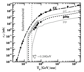
Figure 6: Neutral pion production cross section as a function of the projectil kinetic energy per nucleon for $p+\rm{{}^{4}He}$, $p+\rm{{}^{12}C}$ and $\rm{{}^{12}C+^{12}C}$ interactions. The experimental data points are described in the text, whereas the curves are the predictions of Eq. (9). The $p+p\to\pi^{0}$ production cross section is added for comparison.

Figure 6 shows that the parametrization formula presented in Eq. (9) fits very well the experimental data for $T_{p}\leq 100$ A GeV. One can even extrapolate this parametrization to few-hundreds of A GeV without causing large uncertainties, see Fig. 7.

Figure 7 compares the parametrization of the $\pi^{-}$ production cross section with the available $p+\rm{{}^{12}C}\to\pi^{-}$ production yields from different experiments. The superposition model curve is calculated using the pion production yield ratio $R_{pA}$. The average negative pion multiplicity for $p+C$ is calculated as $\left\langle\pi^{-}\right\rangle_{pC}=R_{pC}\,\left\langle\pi^{-}\right\rangle_{pp}$, where $\left\langle\pi^{-}\right\rangle_{pp}$ is taken from Golokhvastov (2001). The ratio $R_{pA}$ is parametrized experimentally as $R_{pA}\approx 0.5+0.58\,\bar{\nu}$ (Elias et al., 1980). The $\bar{\nu}$ is the average number of inelastic interactions and is given by $\bar{\nu}=A\,\sigma_{pp}/\sigma_{pA}\approx 0.66\,A^{0.31}$, where $A$ is the target mass number and $\sigma_{pp}$ and $\sigma_{pA}$ are the absorption cross sections for nucleon–nucleon and nucleon–nucleus interactions, respectively (Elias et al., 1980). It is clear from Fig. 7 that the parametrization and the superposition model are in good agreement for $T_{p}\leq 100$ A GeV. Their differences for $p+\rm{{}^{4}He}$ are less than 15 %.

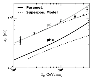
Figure 7: Negativ pion production cross section as a function of projectil kinetic energy per nucleon for $p+\rm{{}^{4}He}$ and $p+\rm{{}^{12}C}$ interactions. The experimental data points are described in the text, the full lines are described by Eq. (9), whereas the dash lines represent the superposition model (Elias et al., 1980) (see the text).

Figure 8 compares the hard photon parametrization formula given in Eq. (8) with the experimental data for $p+\rm{C}$ at $T_{p}=124$ MeV Edgington and Rose (1966) and for $\rm{C+C}$ at $T_{p}=84$ A MeV Grosse et al. (1986). As we can see, the parametrization described here fits reasonably well these experimental data.

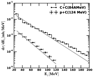
Figure 8: Comparison of the hard photon $\gamma$-ray production differential cross section Eq. (8) with the available experimental data for $p+\rm{{}^{12}C}\to\gamma$ at 124 MeV Edgington and Rose (1966) and $\rm{{}^{12}C+^{12}C}\to\gamma$ at 84 A MeV Grosse et al. (1986).

Figure 9 compares the low energy pion differential cross section parametrization given in Eq. (15) with the available experimental data for $\rm{{}^{14}N+^{27}Al}\to\pi^{0}$ at 35 A MeV (Braun-Munzinger et al., 1984) and $\rm{{}^{12}C+^{12}C}\to\pi^{0}$ at 60, 74 and 84 A MeV Noll et al. (1984). As we can see, the parametrization fits well the data at such energies.

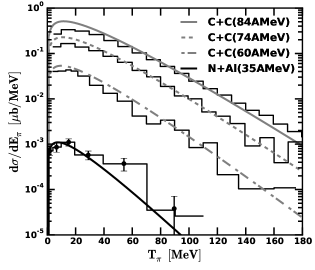
Figure 9: Comparison of the subthreshold $\pi^{0}$ production differential cross section for $\rm{{}^{14}N+^{27}Al}\to\pi^{0}$ at 35 A MeV (Braun-Munzinger et al., 1984) and $\rm{{}^{12}C+^{12}C}\to\pi^{0}$ for 60, 74 and 84 A MeV Noll et al. (1984). The histogram line represent the experimental data, whereas the full line is the parametrization presented in Eq. (15).

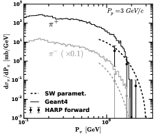
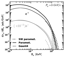
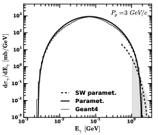
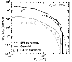
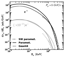
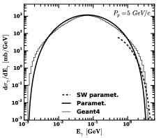
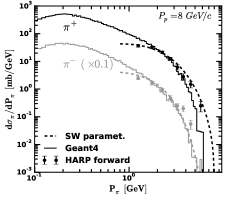
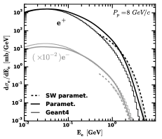
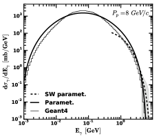
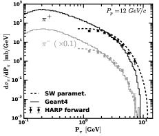
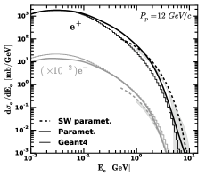
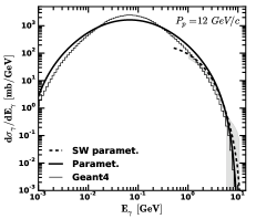
Figure 10: The energy distribution of the $\pi^{\pm}$-mesons and their secondary products created from $p+C$ interactions at $P_{p}=3$, 5, 8, 12 GeV/c. Left column show the $\pi^{\pm}$ energy distribution and the data points are angle integrated HARP forward data Apollonio et al. (2009, 2010). Middle column show the $e^{\pm}$ energy distribution from the $\pi^{\pm}$ decay and the right column show the $\gamma$-ray energy distribution from the $\pi^{0}$ decay. The $\pi^{0}$ differential cross section for the SW parametrization is obtained from the $\pi^{\pm}$ ones through the isospin relations betwee pion species. The histogram lines are the Geant4 predictions, the dash line are the predictions from the angle integrated Sanford-Wang (SW) parametrization (Apollonio et al., 2009) and the full line is the parametrization shown here. The black color in the left and middle columns show the $\pi^{+}$ and $e^{+}$ results, whereas, the gray represent $\pi^{-}$ and $e^{-}$ results. For visual effects, the $\pi^{-}$ results are divided by ten and the $e^{-}$ results are divided by one hundred. The gray areas represent the uncertainties of the $\gamma$-ray and $e^{\pm}$ production spectra when computed directly from the experimental pion data.

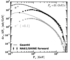
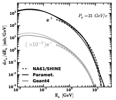
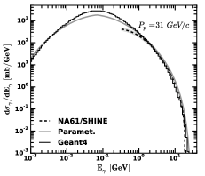
Figure 11: The energy distribution of the $\pi^{\pm}$-mesons and their secondary products created from $p+C$ interactions at $P_{p}=31$ GeV/c. Figure on the left show the $\pi^{\pm}$ energy distribution and the data points are angle integrated NA61/SHINE forward data Abgrall et al. (2011, 2016). Figure in the middle show the $e^{\pm}$ energy distribution from the $\pi^{\pm}$ decay and the figure on the right show the $\gamma$-ray energy distribution from the $\pi^{0}$ decay. The experimental $\pi^{0}$ differential cross section is obtained from the $\pi^{\pm}$ ones through the isospin relations. The histogram lines are the Geant4 predictions, the dash line are the predictions from fitting the $\pi^{\pm}$ forward data and the full line is the parametrization shown here. The black color on the left and middle figures show the $\pi^{+}$ and $e^{+}$ results, whereas, the gray represent the $\pi^{-}$ and $e^{-}$ results. For visual effects, the $\pi^{-}$ results are divided by ten and the $e^{-}$ results are divided by one hundred.

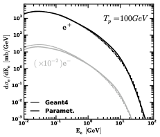
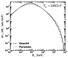
Figure 12: Secondary particles energy distribution for $p+\rm{{}^{12}C}$ interaction at $T_{p}=100$ GeV. The histogram line represent the Geant4 results, whereas the full line is the parametrization presented here. The black lines in the left figure represent the $e^{+}$ results, whereas, the gray color represents the $e^{-}$ results that for visual effects are divided by one hundred.

For collision energies $1\leq T_{p}\leq 100$ A GeV, the parametrization assumes similar secondary particle production spectra for $A+B$ and nucleon–nucleon interactions. To test this assumption Figs. 10–12 compare the results of the parametrization with the HARP and NA61/SHINE forward pion production experimental data (Apollonio et al., 2009, 2010; Abgrall et al., 2011, 2016) and the results of the Geant4.10 Monte Carlo code (Agostinelli et al., 2003; Allison et al., 2006). The hadronic model used in Geant4 simulations is the FTFP-BERT which combines the Bertini intranuclear cascade model at low energies and the FRITIOF string model at higher energies. These comparisons give a good estimate how well the parametrization describes the forward data and how well does it compare with more sophisticated hadronic monte carlo models.

Figures 10 and 11 compare the energy distribution for: $p+C\to\pi^{\pm}$ (left column), $\pi^{\pm}\to e^{\pm}$ decay (middle column) and $\pi^{0}\to\gamma$-ray decay (right column) for collision momenta $P_{p}=3$, 5, 8, 12 and 31 GeV/c. The experimental data points for the $\pi^{\pm}$ energy distributions are obtained from the angular integration of the invariant cross section data Apollonio et al. (2009, 2010); Abgrall et al. (2011, 2016). The histogram lines are the respective results from Geant4 simulations, whereas, the dash lines are the results of the angular integration of the Sanford–Wang (SW) parametrization of the forward pion production invariant cross section (Apollonio et al., 2009). The dash line at $P_{p}=31$ GeV/c are the results of the direct fit of the experimental data. The gray areas represent the uncertainties of the $\gamma$-ray and $e^{\pm}$ production spectra when computed directly from the experimental pion data.

The left column of Figs 10 and 11 compare the forward $\pi^{\pm}$ spectral data with Geant4 predictions. It is clear from the figures that the Geant4 overestimates the forward pion production data for $P_{p}=3$ and 5 GeV/c and it agrees reasonably well for $P_{p}>5$ GeV/c. The SW parametrization also overestimates the $\pi^{+}$ production at $P_{p}=3$ GeV/c and it does not satisfy the kinematic limit, i.e. have non-zero cross sections for pion energy greater than the maximum allowed by the kinematics.

The full lines in the middle and right columns of Figs. 10 and 11 represent predictions from the parametrization developed here. The $\gamma$-ray energy distribution that is presented with dash lines, are computed from $\pi^{\pm}$ cross sections:

$$\frac{d\sigma_{\pi^{0}}}{dE_{\pi^{0}}}=\frac{1}{2}\left(\frac{d\sigma_{\pi^{+}}}{dE_{\pi^{+}}}+\frac{d\sigma_{\pi^{-}}}{dE_{\pi^{-}}}\right),$$

where the $d\sigma_{\pi^{\pm}}/dE_{\pi^{\pm}}$ are the angle integrated forward data or the SW parametrization.

From the left column of Figs. 10 and 11, we see that the forward experimental pion data agree with Geant4 predictions for $E_{\pi}>1$ GeV. This means that lower energy pion production is a result of large-angle emission. When comparing the $\gamma$-ray and $e^{\pm}$ energy distributions in the forward region above 1 GeV, good agreements are found between the experimental data plotted with the gray area and the SW parametrization, Geant4 and the parametrization developed here. The deviations are expected for energies below 1 GeV. We can see that the parametrization and the Geant4 predictions agree reasonably well for the $\pi^{0}\to 2\gamma$ energy distribution. The maximum deviation is of the order 30–40 %. For the $e^{\pm}$ energy distributions the deviations between these two models are larger. For $P_{p}\leq 5$ GeV/c, the $e^{-}$ production spectra between these two models agree reasonably well, whereas, the $e^{+}$ spectra disagree by a factor as large as three. For $P_{p}>5$ GeV/c the $e^{+}$ spectra agrees reasonably good between these two models and disagree for the $e^{-}$ spectra by a factor as large as two. The root of these disagreements however, seem to be related with the total $e^{\pm}$ production yield. The parametrization developed here fits well the experimental pion yield data, thus, I believe that these large disagreements are not a result of the assumption of similar $e^{\pm}$ spectra between $p+$C and nucleon–nucleon.

As a last example, Fig. 12 compares the $p+C$ secondary particle production at $T_{p}=100$ GeV between Geant4 and the parametrization introduced here. These two models agree reasonably well at this collision energy with differences less than 35 %.

VI Results and Discussion

To illustrate the results of the parametrizations developed here, let us consider two examples. The first one considers $p$ and ¹²C projectiles interacting with the ¹²C target material. The projectile fluxes are described in one case by a power-law function with index $\alpha=3$ and, in the second case by the same power-law but with an exponential cut-off at $T_{p}^{\rm cut}=1$ A GeV. In the second example, the chemical composition of both projectiles and target material are considered to be similar to the solar composition of elements. The projectile fluxes for this example are assumed to be in one case a pure power-law function with index varying between $2\leq\alpha\leq 5$, whereas, in the second case the same power-law function but with an exponential cut-off at $T_{p}^{\rm cut}=1$ A GeV.

Consider the following functional form for the projectile flux:

$$J_{A}(T_{p})=\mathcal{N}\times T_{p}^{-\alpha}\times\exp\left(-\frac{T_{p}}{T_{p}^{\rm cut}}\right).$$ (23)

Assuming that the target number density is $n_{B}$, the $\gamma$-ray production spectrum is given by:

$$\frac{dN}{dE_{\gamma}}=4\pi\,n_{B}\int\limits_{T_{p}^{\rm th}}^{\infty}dT_{p}\;J_{A}(T_{p})\;\frac{d\sigma_{\gamma}^{AB}}{dE_{\gamma}}(T_{p},E_{\gamma}).$$ (24)

Here, $d\sigma_{\gamma}^{AB}/dE_{\gamma}$ is the sum of the $\gamma$-ray production cross sections via formation of hard photons ($A+B\to\gamma$) and decay of secondary $\pi^{0}$-mesons ($A+B\to\pi^{0}$). $T_{p}^{\rm th}$ is the kinematic threshold kinetic energy per nucleon. For $\pi^{0}$ production $T_{p}^{\rm th}$ is given by Eq. (13). For producing hard photons with $E_{\gamma}\geq E_{\gamma}^{\rm min}=30$ MeV it is given by:

$$T_{p}^{\rm th}=\left(\frac{1}{A_{p}}+\frac{1}{A_{t}}\right)E_{\gamma}^{\rm min},$$

where, $A_{p}$ and $A_{t}$ are the mass numbers for the projectile $A$ and the target $B$, respectively. The $e^{\pm}$ pair production spectra is calculated using Eqs. (21, 22 and 23).

Calculation of the $\gamma$-ray spectrum for a solar-like composition of elements, includes a sum over all possible nuclear collisions. Let $n_{B}$ be the element $B$ number density in the target material and $J_{A}$ be the projectile $A$ flux defined in Eq. (23). In addition, let us assume that all projectiles fluxes have the same $\alpha$ and $T_{p}^{\rm cut}$ parameters. If we note with $X_{p}^{A}=J_{A}/J_{p}$ the flux ratio between the element $A$ and the proton, and $X_{t}^{B}=n_{B}/n_{H}$ the target number density ratio between the element $B$ and hydrogen, then the Eq. (24) transforms to:

$$\frac{dN}{dE_{\gamma}}=\mathcal{C}\sum\limits_{A,B}X_{p}^{A}\,X_{t}^{B}\!\!\!\!\!\!\int\limits_{T_{p}^{\rm th}(AB)}^{\infty}\!\!\!\!\!\!\!\!dT_{p}\;J(T_{p})\frac{d\sigma_{\gamma}^{AB}}{dE_{\gamma}}(T_{p},E_{\gamma}).$$ (25)

Here, $T_{p}^{\rm th}(AB)$ is the threshold energy for the specific $A+B$ interaction, $J=J_{A}/\mathcal{N}_{A}$ is the same for all projectiles, and $\mathcal{C}=4\pi\,n_{p}\,\mathcal{N}_{p}$ is a normalization constant. When using this formula it is important to recall that the hard photon cross section is calculated for projectiles lighter or equal the mass of the target nucleus. Therefore, the contribution of $A+B$, when $A$ is heavier than $B$, is calculated from $B+A$.

For a solar-like composition of elements: H, ⁴He, ¹²C, ¹⁴N, ¹⁶O, ²⁰Ne, ²⁴Mg, ²⁸Si, ³²S and ⁵⁶Fe, we have $X_{p}=X_{t}=1:9.59\times 10^{-2}:4.65\times 10^{-4}:8.3\times 10^{-5}:8.3\times 10^{-4}:1.2\times 10^{-4}:3.87\times 10^{-5}:3.69\times 10^{-5}:1.59\times 10^{-5}:3.25\times 10^{-5}$ (see e.g. Meyer, 1985).

At higher energies nucleus–nucleus and $pp$ $\gamma$-ray spectral shape are similar, therefore, by using the wounded nucleon model (Białłas et al., 1976) we can scale the $\gamma$-ray spectra from $pp$ interactions with the following factor:

$$\epsilon=\sum\limits_{A,B}X_{p}^{A}\,X_{t}^{B}\,\frac{\sigma_{R}(AB)\,W_{AB}}{2\,\sigma_{pp}}.$$ (26)

Where, $\sigma_{R}(AB)$ is the reaction cross section for $A+B$ interactions, see Eq. (2). $W_{AB}=(A_{p}\,\sigma_{pB}+A_{t}\,\sigma_{pA})/\sigma_{AB}$ is the number of wounded nucleons and $\sigma_{pA}$, $\sigma_{pB}$ and $\sigma_{AB}$ are the inelastic $p+A$, $p+B$ and $A+B$ cross sections calculated using parametrization (Shen et al., 1989). The $\sigma_{pp}$ is the $pp$ inelastic cross section and is taken from (Kafexhiu et al., 2014).

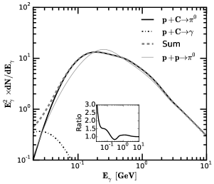
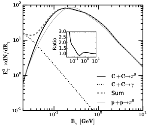
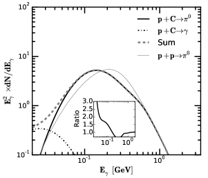
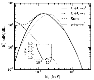
Figure 13: Gamma-ray production spectra for $p+^{12}$C (left) and ¹²C+¹²C (right) interactions. The projectile fluxes have a power-law index $\alpha=3$ and in one case $T_{p}^{\rm cut}\to\infty$ (top) and in the other case $T_{p}^{\rm cut}=1$ A GeV (bottom), see Eq. (23). The thick black line is the $\pi^{0}\to 2\gamma$ contribution, doted line is the hard photon contribution and the dash line is the sum. The thin gray line correspond to $pp\to\pi^{0}$ scaled according to the wounded nucleon model. The small panel in each plot show the spectral ratio between the nucleus–nucleus and $pp$.

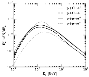
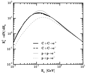
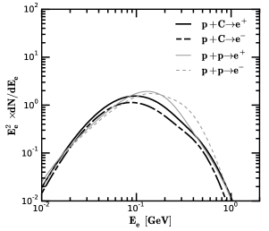
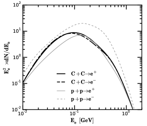
Figure 14: Electron and positron production spectra for $p+^{12}$C (left) and ¹²C+¹²C (right) interactions. The projectile fluxes have a power-law index $\alpha=3$ and in one case $T_{p}^{\rm cut}\to\infty$ (top) and in the other case $T_{p}^{\rm cut}=1$ A GeV (bottom), see Eq. (23). The thick black line corresponds to $e^{+}$ production and the thick dash-line correspond to $e^{-}$ production. The thin gray line shows the contribution from $pp\to e^{+}$ and the thin dash-doted line shows the contribution from $pp\to e^{-}$ which are scaled for each case according to the wounded nucleon model.

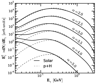
Figure 15: Gamma-ray production spectrum from the hard photons and $\pi^{0}$-meson decay for a solar-like composition of elements. The exponential cut-off energies are $T_{p}^{\rm cut}\to\infty$ (left) and $T_{p}^{\rm cut}=1$ A GeV (right), whereas, the power-law index varies between $2\leq\alpha\leq 5$. The solid lines represent the contribution from all nuclei, whereas, the thin dash lines represent the $\gamma$-ray spectra from $pp$ collisions which are scaled according to the wounded nucleon model.

Figures 13 and 14 show the $\gamma$-ray and $e^{\pm}$ spectra resulting from $p+^{12}$C and ¹²C+¹²C interactions. Looking at these figures, one can draw some general conclusions that are related to subthreshold pions and hard photon production: The $pp$ interactions fail to reproduce the $A+B$ secondary particle shape below 1 GeV. The $A+B$ interactions produce a secondary particle spectra that is generally broader than the respective $pp$ one. Direct hard photons manifest themselves for $E_{\gamma}<100$ MeV and this component produce a unique feature in the final $\gamma$-ray spectrum that has no analogue in $pp$ interactions. Finally, the differences between $A+B$ and $pp$ secondary particle production spectra depends on the nuclear mass and it increases when the masses increase.

The presence of a low energy exponential cut-off suppresses the high energy collisions. As a result, the relative contribution of hard photons and subthreshold pions increases. The low energy cut-off creates two effects: Firstly, it increases the relative $\gamma$-ray production rate for $E_{\gamma}<200$ MeV, which is unique for nuclear interactions, see Fig 13. Secondly, the peak of the $\gamma$-ray and $e^{\pm}$ spectra produced from nuclear interactions shifts toward lower energies at a higher rate compared to $pp$ interactions. For the $\alpha=3$ and $T_{p}^{\rm cut}=1$ A GeV example that was considered here, the peak energy of the secondary spectra computed from nuclear collisions is about 40 % smaller than that of the $pp$, see Fig. 13 and 14.

Independent of the projectile flux, the $\gamma$-ray spectrum for $E_{\gamma}<100$ MeV between $p+^{12}{\rm C}$ and ¹²C+${}^{12}{\rm C}$ is different. This is due to different hard photon production cross sections between these two nuclear interactions. The ¹²C+${}^{12}{\rm C}$ hard photon production cross section is larger and its spectrum is harder compared to $p+^{12}{\rm C}$. Therefore, the shape of the spectrum for $E_{\gamma}<100$ MeV can be used to discriminate not only $pp$ from nuclear collisions but also between different nucleus–nucleus interactions and it can be used in this way to estimate the mass of the colliding nuclei.

Proton–proton interactions produce $\pi^{+}$ for collision energies $T_{p}>0.28$ GeV and $\pi^{-}$ for $T_{p}>1.2$ GeV. Nucleus–nucleus interactions on the other hand, produce $\pi^{\pm}$ at much lower energies and with equal amount. This is a consequence of the isospin symmetry and having equal number of protons and neutrons in both projectile and target nuclei. Therefore, nuclear interactions produce similar amounts of $e^{+}$ and $e^{-}$ with similar spectral shape, in contrast to $pp$ interactions, which produce an excess of $e^{+}$ compared to $e^{-}$ at low energies. The exponential cut-off at $T_{p}^{\rm cut}=1$ A GeV suppresses the $p+p\to e^{-}$ production and because of this, its shape is very different when compared with $A+B\to e^{-}$ spectrum, see Figure 14. For $p+^{12}$C interaction, the projectile has no neutrons and as a result, the amount of $\pi^{+}$ ($e^{+}$) would be slightly larger than $\pi^{-}$ ($e^{-}$).

Figure 15 shows the results for a solar composition of elements. The discussion about $p+^{12}{\rm C}$ and ¹²C+${}^{12}{\rm C}$ interactions is also valid here. Furthermore, these calculations show that high energy nuclear interactions that result from hard spectrum of projectiles, produce abundant low energy $\gamma$-rays that screen the contribution of subthreshold pions and hard photons. Thus, the $\gamma$-ray spectrum from $A+B$ collisions with a primary spectrum harder than $\alpha\lesssim 2.5$, show no difference from $pp$. On the other hand, softer primary spectra and low energy cut-off produce significant differences between $A+B$ and $pp$ final $\gamma$-ray spectra below 200 MeV. This can be important in many astrophysical situations such as solar flares and oxygen-rich supernova remnants where soft ion spectra are produced and one cannot extrapolate $pp$ calculations for $E_{\gamma}\leq 200$ MeV.

VII Summary and Conclusions

In this work, using numerous publicly available experimental data sets, simple and reasonably accurate parametrization formulas are provided to calculate the $\gamma$-ray and $e^{\pm}$ pair production spectra for nucleus–nucleus interactions with collision energy $T_{p}\leq 100$ A GeV including the low energy subthreshold pion and hard photon channels. The parametrizations are in reasonably good agreement with the available experimental data and the expected deviations are less than 30–40 %. These parametrizations are provided in the form of a computer library in (Kafexhiu, 2016).

I conclude by stressing the importance of the subthreshold pion and hard photon channels for computing the secondary particle production spectra from low energy nuclear collisions. The $\gamma$-ray spectra produced by these two channels below 200 MeV cannot be reproduced by $pp$ interactions. This characteristic feature can be used to experimentally distinguish the contribution of nuclei from protons. While the detection of $\gamma$-rays for $E_{\gamma}\gtrsim 1$ GeV can be used to fix the primary spectra parameters, the detection of $E_{\gamma}\lesssim 200$ MeV can be used to estimate the masses of the colliding nuclei. Gamma-ray instruments, such as Fermi-LAT, that are sensitive in this energy region should include the contribution of these two channels in their $\gamma$-ray analysis especially for astrophysical sources that have soft primary nuclear spectra.

Future work will improve the accuracy of the pion energy distribution. This is possible if at low energies a two temperature pion spectra is considered instead of one. At high energies one could parametrize the pion spectrum directly from the proton–nucleus and nucleus–nucleus experimental data.

Appendix A Calculation of the pion energy distribution using $pp$ cross sections

High energy $A+B$ inelastic collisions produce pions through $pp$, $np$ and $nn$ interactions. The average pion yield from these individual interactions are different, therefore, a correct estimation of the pion production cross section from nucleus–nucleus collisions should average over different nucleon–nucleon contributions. Let the $Z_{p}$, $A_{p}$ and $Z_{t}$ and $A_{t}$ be the number of protons and the total number of nucleons for the projectile $A$ and the target $B$. Let us define $\xi_{p}=Z_{p}/A_{p}$ and $\xi_{t}=Z_{t}/A_{t}$ the probabilities of randomly colliding with a proton inside the projectile and the target nuclei, respectively. The quantities $1-\xi_{p}$ and $1-\xi_{t}$ express the probabilities for colliding with a neutron. Using these probabilities, the average pion multiplicity per nucleon–nucleon collision is:

$$\begin{split}\left\langle\pi_{NN}\right\rangle=\xi_{p}\xi_{t}\left\langle\pi_{pp}\right\rangle\!&+\![\xi_{p}(1-\xi_{t})+\xi_{t}(1-\xi_{p})]\left\langle\pi_{np}\right\rangle\\ &+(1-\xi_{p})(1-\xi_{t})\left\langle\pi_{nn}\right\rangle,\end{split}$$ (27)

where, $\left\langle\pi_{pp}\right\rangle$, $\left\langle\pi_{np}\right\rangle$ and $\left\langle\pi_{nn}\right\rangle$ are the pion average production multiplicities for $pp$, $np$ and $nn$ collisions, respectively. The multiplicity for $A+B$ collisions is $\left\langle\pi_{AB}\right\rangle\sim\left\langle\pi_{NN}\right\rangle$ and the proportionality factor is the number of participating nucleons.

Assuming that charge and isospin symmetries hold at $T_{p}>1$ A GeV, then the average pion production multiplicities satisfy the following relations (see e.g. Golokhvastov, 2001):

$$\begin{array}[]{l}\left\langle\pi_{pp}^{-}\right\rangle=\left\langle\pi_{nn}^{+}\right\rangle\\ \left\langle\pi_{pp}^{0}\right\rangle=\left\langle\pi_{nn}^{0}\right\rangle=\left\langle\pi_{np}^{\pm,0}\right\rangle\\ \left\langle\pi_{pp}^{+}\right\rangle=\left\langle\pi_{nn}^{-}\right\rangle\\ \end{array}$$ (28)

From these relations follows that $\left\langle\pi_{pp}^{0}\right\rangle=\left(\left\langle\pi_{pp}^{+}\right\rangle+\left\langle\pi_{pp}^{-}\right\rangle\right)/2$ which is used in the text. Moreover, assuming that these relations extent to differential cross sections, then, by manipulating Eqs. (27 and 28) follows that:

$$\begin{array}[]{l}f_{AB}^{\pi^{+}}=\left(\frac{\xi_{p}+\xi_{t}}{2}\right)\times f_{pp}^{\pi^{+}}+\left(1-\frac{\xi_{p}+\xi_{t}}{2}\right)\times f_{pp}^{\pi^{-}},\\ \\ f_{AB}^{\pi^{0}}=f_{pp}^{\pi^{0}},\\ \\ f_{AB}^{\pi^{-}}=\left(1-\frac{\xi_{p}+\xi_{t}}{2}\right)\times f_{pp}^{\pi^{+}}+\left(\frac{\xi_{p}+\xi_{t}}{2}\right)\times f_{pp}^{\pi^{-}},\\ \end{array}$$ (29)

where, $f=\sigma_{\rm inel}^{-1}\times d\sigma/dE_{\pi}$ is the pion energy distribution for $A+B$ and $pp$ interactions. These relations are used to calculate the $A+B\to(e^{\pm},~{}\gamma)$ energy distribution using $p+p\to(e^{\pm},~{}\gamma)$ parametrizations.

References

- Grimm and Grosse (1985) P. Grimm and E. Grosse, Progress in Particle and Nuclear Physics 15, 339 (1985).
- Grosse (1986) E. Grosse, Nuclear Physics A 447, 611 (1986).
- Nifenecker and Pinston (1989) H. Nifenecker and J. A. Pinston, Progress in Particle and Nuclear Physics 23, 271 (1989).
- Cassing et al. (1990) W. Cassing, V. Metag, U. Mosel, and K. Niita, Phys. Rep. 188, 363 (1990).
- Schutz et al. (1997) Y. Schutz, G. Martínez, F. M. Marqués, A. Marín, T. Matulewicz, R. W. Ostendorf, P. Bożek, H. Delagrange, J. Díaz, M. Franke, et al., Nuclear Physics A 622, 404 (1997).
- D’Enterria and Martínez (2000) D. G. D’Enterria and G. Martínez, Czechoslovak Journal of Physics 50, 103 (2000), eprint nucl-ex/0007005.
- D’Enterria et al. (2001) D. G. D’Enterria, L. Aphecetche, A. Chbihi, H. Delagrange, J. Díaz, M. J. van Goethem, M. Hoefman, A. Kugler, H. Löhner, G. Martínez, et al., Physical Review Letters 87, 022701 (2001), eprint nucl-ex/0012009.
- Stock (1986) R. Stock, Phys. Rep. 135, 259 (1986).
- Senger and Ströbele (1999) P. Senger and H. Ströbele, Journal of Physics G Nuclear Physics 25, 59 (1999), eprint nucl-ex/9810007.
- Bonasera et al. (2006) A. Bonasera, R. Coniglione, and P. Sapienza, European Physical Journal A 30, 47 (2006).
- Glauber (1955) R. J. Glauber, Physical Review 100, 242 (1955).
- Franco and Glauber (1966) V. Franco and R. J. Glauber, Physical Review 142, 1195 (1966).
- Glauber and Matthiae (1970) R. J. Glauber and G. Matthiae, Nuclear Physics B 21, 135 (1970).
- Białłas et al. (1976) A. Białłas, M. Bleszyński, and W. Czyż, Nuclear Physics B 111, 461 (1976).
- Bialas et al. (1977) A. Bialas, W. Czyz, and W. Furmanski, Acta Phys. Polon. B8, 585 (1977).
- Anisovich et al. (1978) V. V. Anisovich, Y. M. Shabelsky, and V. M. Shekhter, Nuclear Physics B 133, 477 (1978).
- Nikolaev (1981) N. N. Nikolaev, Sov. Phys. Usp. 24, 531 (1981), [Usp. Fiz. Nauk134,369(1981)].
- Gaisser and Schaefer (1992) T. K. Gaisser and R. K. Schaefer, ApJ 394, 174 (1992).
- Bertholet et al. (1987) R. Bertholet, M. Kwato Njock, M. Maurel, E. Monnand, H. Nifenecker, P. Perrin, J. A. Pinston, F. Schussler, D. Barneoud, C. Guet, et al., Nuclear Physics A 474, 541 (1987).
- Nifenecker and Bondorf (1985) H. Nifenecker and J. P. Bondorf, Nuclear Physics A 442, 478 (1985).
- Breitbach et al. (1989) G. Breitbach, G. Koch, S. Koch, W. Kühn, A. Ruckelshausen, V. Metag, R. Novotny, S. Riess, D. Habs, D. Schwalm, et al., Phys. Rev. C 40, 2893 (1989).
- Gossett et al. (1990) C. A. Gossett, J. A. Behr, S. J. Luke, B. T. McLain, D. P. Rosenzweig, K. A. Snover, and W. T. Hering, Phys. Rev. C 42, 1800 (1990).
- Stevenson et al. (1986) J. Stevenson, K. B. Beard, W. Benenson, J. Clayton, E. Kashy, A. Lampis, D. J. Morrissey, M. Samuel, R. J. Smith, C. L. Tam, et al., Physical Review Letters 57, 555 (1986).
- Martínez et al. (1995) G. Martínez, F. M. Marqués, Y. Schutz, G. Wolf, J. Díaz, M. Franke, S. Hlaváč, R. Holzmann, P. Lautridou, F. Lefévre, et al., Physics Letters B 349, 23 (1995).
- Tam et al. (1988) C. L. Tam, J. Stevenson, W. Benenson, J. Clayton, Y. Chen, E. Kashy, A. R. Lampis, D. J. Morrissey, M. Samuel, T. K. Murakami, et al., Phys. Rev. C 38, 2526 (1988).
- Tam et al. (1989) C. L. Tam, J. Stevenson, W. Benenson, J. Clayton, Y. Chen, E. Kashy, A. R. Lampis, D. J. Morrissey, M. Samuel, T. K. Murakami, et al., Phys. Rev. C 39, 1371 (1989).
- Njock et al. (1986) M. K. Njock, M. Maurel, E. Monnand, H. Nifenecker, J. Pinston, F. Schussler, and D. Barneoud, Physics Letters B 175, 125 (1986).
- Hingmann et al. (1987) R. Hingmann, W. Kühn, V. Metag, R. Mühlhans, R. Novotny, A. Ruckelshausen, W. Cassing, H. Emling, R. Kulessa, H. J. Wollersheim, et al., Physical Review Letters 58, 759 (1987).
- Grosse et al. (1986) E. Grosse, P. Grimm, H. Heckwolf, W. F. J. Müller, H. Noll, A. Oskarsson, H. Stelzer, and W. Rösch, EPL (Europhysics Letters) 2, 9 (1986).
- Martínez et al. (1994) G. Martínez, J. Díaz, M. Franke, S. Hlaváč, R. Holzmann, P. Lautridou, F. Lefèvre, H. Löhner, A. Marín, M. Marqués, et al., Physics Letters B 334, 23 (1994).
- Njock et al. (1988) M. K. Njock, M. Maurel, E. Monnand, H. Nifenecker, P. Perrin, J. A. Pinston, F. Schussler, and Y. Shutz, Nuclear Physics A 489, 368 (1988).
- Clayton et al. (1989) J. Clayton, J. Stevenson, W. Benenson, Y. Chen, E. Kashy, A. R. Lampis, M. Samuel, C. L. Tam, M. F. Mohar, D. J. Morrissey, et al., Phys. Rev. C 40, 1207 (1989).
- Schubert et al. (1994) A. Schubert, R. Holzmann, S. Hlaváč, R. Kulessa, W. Niebur, R. S. Simon, P. Lautridou, F. Lefèvre, M. Marqués, T. Matulewicz, et al., Physical Review Letters 72, 1608 (1994).
- Edgington and Rose (1966) J. A. Edgington and B. Rose, Nucl. Phys. A 89, 523 (1966).
- Martínez et al. (1999) G. Martínez, Y. Charbonnier, L. Aphecetche, H. Delagrange, K. K. Gudima, T. Matulewicz, M. Ploszajczak, Y. Schutz, V. Toneev, R. Turrisi, et al., Physical Review Letters 83, 1538 (1999).
- Metag (1993) V. Metag, Nuclear Physics A 553, 283 (1993).
- Hüfner and Knoll (1977) J. Hüfner and J. Knoll, Nuclear Physics A 290, 460 (1977).
- Cugnon et al. (1981) J. Cugnon, J. Knoll, and J. Randrup, Nuclear Physics A 360, 444 (1981).
- Golokhvastov (2001) A. I. Golokhvastov, Physics of Atomic Nuclei 64, 1841 (2001).
- Bellini et al. (1989) V. Bellini, M. Boloré, J. Julien, J. M. Hisleur, A. Fallica, A. S. Figuera, R. Fonte, A. Insolia, C. Milone, G. F. Palama, et al., Zeitschrift fur Physik A Hadrons and Nuclei 333, 393 (1989).
- Bayukov et al. (1957) Y. D. Bayukov, M. S. Kozodayev, Y. D. Prokoshkin, and A. A. Tyapkin, Nucl. Phys. A 4, 61 (1957).
- Dunaitsev and Prokoshkin (1964) A. F. Dunaitsev and Y. D. Prokoshkin, Nucl. Phys. A 56, 300 (1964).
- Pollack and Fazio (1963) J. B. Pollack and G. G. Fazio, Physical Review 131, 2684 (1963).
- Waters et al. (1993) M. Waters, H. Machner, D. Gotta, K. Kilian, P. Turek, D. Grzonka, G. Gaul, R. Santo, T. Manz, J. Ernst, et al., Nuclear Physics A 564, 595 (1993).
- Braun-Munzinger et al. (1984) P. Braun-Munzinger, P. Paul, L. Ricken, J. Stachel, P. H. Zhang, G. R. Young, F. E. Obenshain, and E. Grosse, Physical Review Letters 52, 255 (1984).
- Julien et al. (1988) J. Julien, M. Boloré, H. Dabrowski, J. M. Hisleur, V. Bellini, A. S. Figuera, R. Fonte, A. Insolia, G. F. Palama, G. V. Russo, et al., Zeitschrift fur Physik A Hadrons and Nuclei 330, 83 (1988).
- Heckwolf et al. (1984) H. Heckwolf, E. Grosse, H. Dabrowski, O. Klepper, C. Michel, W. F. J. Müller, H. Noll, C. Brendel, W. Rösch, J. Julien, et al., Zeitschrift fur Physik A Hadrons and Nuclei 315, 243 (1984).
- Noll et al. (1984) H. Noll, E. Grosse, P. Braun-Munzinger, H. Dabrowski, H. Heckwolf, O. Klepper, C. Michel, W. F. J. Müller, H. Stelzer, C. Brendel, et al., Physical Review Letters 52, 1284 (1984).
- Badalá et al. (1993) A. Badalá, R. Barbera, A. Palmeri, G. S. Pappalardo, F. Riggi, A. C. Russo, C. Agodi, R. Alba, G. Bellia, R. Coniglione, et al., Phys. Rev. C 47, 231 (1993).
- Badalà et al. (1996) A. Badalà, R. Barbera, A. Palmeri, G. S. Pappalardo, F. Riggi, A. C. Russo, G. Russo, and R. Turrisi, Phys. Rev. C 53, 1782 (1996).
- Moisan et al. (1992) C. Moisan, N. De Takacsy, J. Barrette, S. K. Mark, G. Ingold, J. Stachel, P. Braun-Munzinger, N. Alamanos, Y. Cassagnou, J. M. Hisleur, et al., Nuclear Physics A 537, 667 (1992).
- Schwalb et al. (1994) O. Schwalb, M. Pfeiffer, F.-D. Berg, M. Franke, W. Kühn, V. Metag, M. Notheisen, R. Novotny, J. Ritman, M. E. Röbig-Landau, et al., Physics Letters B 321, 20 (1994).
- Holzmann et al. (1997) R. Holzmann, M. Appenheimer, R. Averbeck, Y. Charbonnier, H. Delagrange, J. Díaz, A. Döppenschmidt, V. Hejny, S. Hlaváč, A. Kugler, et al., Phys. Rev. C 56, 2920 (1997).
- Averbeck et al. (2003) R. Averbeck, R. Holzmann, V. Metag, and R. S. Simon, Phys. Rev. C 67, 024903 (2003), eprint nucl-ex/0012007.
- Laue et al. (2000) Laue, I. Böttcher, M. Debowski, A. Förster, E. Grosse, P. Koczoń, B. Kohlmeyer, M. Mang, M. Menzel, L. Naumann, et al., European Physical Journal A 9, 397 (2000), eprint nucl-ex/0011010.
- Badala et al. (1992) A. Badala, R. Barbera, A. Palmeri, G. Pappalardo, A. Bonasera, et al., Phys.Rev. C46, 604 (1992).
- Crawford et al. (1980) J. F. Crawford, M. Daum, G. H. Eaton, R. Frosch, H. Hirschmann, R. Horisberger, J. W. McCulloch, E. Steiner, R. Hausammann, R. Hess, et al., Phys. Rev. C 22, 1184 (1980), URL http://link.aps.org/doi/10.1103/PhysRevC.22.1184.
- Abbott et al. (1992) T. Abbott, Y. Akiba, D. Beavis, M. A. Bloomer, P. D. Bond, C. Chasman, Z. Chen, Y. Y. Chu, B. A. Cole, J. B. Costales, et al., Phys. Rev. D 45, 3906 (1992).
- Whitmore et al. (1994) J. J. Whitmore, F. Persi, W. S. Toothacker, P. A. Elcombe, J. C. Hill, W. W. Neale, W. D. Walker, W. Kowald, P. Lucas, L. Voyvodic, et al., Zeitschrift fur Physik C Particles and Fields 62, 199 (1994).
- Agakishiyev et al. (1985) H. N. Agakishiyev, N. Akhababian, D. Armutlijsky, A. M. Baldin, J. Bartke, R. Bekmirsaev, J. Bogdanowicz, A. P. Cheplakov, L. A. Didenko, A. P. Gasparian, et al., Zeitschrift fur Physik C Particles and Fields 27, 177 (1985).
- Aksinenko et al. (1980) V. D. Aksinenko, M. K. Anikina, V. S. Buttsev, L. V. Chkaidze, N. S. Glagoleva, A. I. Golokhvastov, A. G. Grachov, K. K. Gudima, E. A. Dementjev, S. V. Kadikova, et al., Nuclear Physics A 348, 518 (1980).
- Baatar et al. (1980) T. Baatar, A. Gasparian, G. Gafurov, N. Grigalashvili, S. Korchagin, et al., Yad.Fiz. 32, 1372 (1980).
- Armutliisky et al. (1988) D. Armutliisky, N. Akhababian, V. Grishin, I. Ivanovskaya, and E. Kladnitskaya, Sov.J.Nucl.Phys. 48, 101 (1988).
- Miller and Nowak (1975) D. J. Miller and E. Nowak, Lettere al Nuovo Cimento (1971-1985) 13, 39 (1975), ISSN 1827-613X, URL http://dx.doi.org/10.1007/BF02742565.
- Brick et al. (1989) D. H. Brick, M. Widgoff, P. Beilliere, P. Lutz, J. L. Narjoux, N. Gelfand, E. D. Alyea, Jr., M. Bloomer, J. Bober, W. Busza, et al., Phys. Rev. D 39, 2484 (1989).
- Johansson et al. (1982) T. Johansson, H.-Å. Gustafsson, B. Jakobsson, P. Kristiansson, B. Norén, A. Oskarsson, L. Carlén, I. Otterlund, H. Ryde, J. Julien, et al., Physical Review Letters 48, 732 (1982).
- Müntz et al. (1997) C. Müntz, P. Baltes, H. Oeschler, C. Sartorius, C. Sturm, A. Wagner, C. Bormann, D. Brill, Y. Shin, J. Stein, et al., Zeitschrift fur Physik A Hadrons and Nuclei 357, 399 (1997).
- Young et al. (1986) G. R. Young, F. E. Obenshain, F. Plasil, P. Braun-Munzinger, R. Freifelder, P. Paul, and J. Stachel, Phys. Rev. C 33, 742 (1986).
- Piasecki et al. (2010) K. Piasecki, T. Matulewicz, N. Yahlali, H. Delagrange, J. Díaz, D. G. D’Enterria, F. Fernández, A. Kugler, H. Löhner, G. Martínez-García, et al., Phys. Rev. C 81, 054912 (2010), eprint 0909.1673.
- Mayer et al. (1993) R. S. Mayer, W. Henning, R. Holzmann, R. S. Simon, H. Delagrange, F. Lefèvre, T. Matulewicz, R. Merrouch, W. Mittig, R. W. Ostendorf, et al., Physical Review Letters 70, 904 (1993).
- Marín et al. (1997) A. Marín, J. Díaz, R. Averbeck, S. Hlaváč, R. Holzmann, F. Lefèvre, A. Schubert, R. S. Simon, Y. Charbonnier, G. Martínez, et al., Physics Letters B 409, 77 (1997).
- Suzuki et al. (1991) T. Suzuki, M. Fukuda, T. Ichihara, N. Inabe, T. Kubo, T. Nakagawa, K. Yoshida, I. Taniahata, T. Kobayashi, T. Suda, et al., Physics Letters B 257, 27 (1991).
- Brockmann et al. (1984) R. Brockmann, J. W. Harris, A. Sandoval, R. Stock, H. Ströbele, G. Odyniec, H. G. Pugh, L. S. Schroeder, R. E. Renfordt, D. Schall, et al., Physical Review Letters 53, 2012 (1984).
- Nagamiya et al. (1982) S. Nagamiya, H. Hamagaki, P. Hecking, S. Kadota, R. Lombard, Y. Miake, E. Moeller, S. Schnetzer, H. Steiner, I. Tanihata, et al., Physical Review Letters 48, 1780 (1982).
- Backović et al. (1992) S. Backović, D. Salihagić, L. Simić, D. Krpić, S. Drndarević, R. R. Mekhdiyev, A. P. Cheplakov, H. N. Agakishiev, E. N. Kladnitskaya, and S. Y. Sivoklokov, Phys. Rev. C 46, 1501 (1992).
- Chkhaidze et al. (1992) L. Chkhaidze, T. Dzobava, L. Kharkhelauri, I. Tuliani, E. Okonov, G. Vardenga, and G. Taran, Zeitschrift fur Physik C Particles and Fields 54, 179 (1992).
- Barr et al. (2007) G. Barr, O. Chvala, H. G. Fischer, M. Kreps, M. Makariev, C. Pattison, A. Rybicki, D. Varga, and S. Wenig, European Physical Journal C 49, 919 (2007), eprint hep-ex/0606029.
- Andronov and for the NA61/SHINE Collaboration (2015) E. Andronov and for the NA61/SHINE Collaboration, ArXiv e-prints (2015), eprint 1512.05938.
- Kamae et al. (2006) T. Kamae, N. Karlsson, T. Mizuno, T. Abe, and T. Koi, ApJ 647, 692 (2006), eprint astro-ph/0605581.
- Kafexhiu et al. (2014) E. Kafexhiu, F. Aharonian, A. M. Taylor, and G. S. Vila, Phys. Rev. D 90, 123014 (2014), eprint 1406.7369.
- Scanlon and Milford (1965) J. H. Scanlon and S. N. Milford, ApJ 141, 718 (1965).
- Dermer (1986) C. D. Dermer, ApJ 307, 47 (1986).
- Elias et al. (1980) J. E. Elias, W. Busza, C. Halliwell, D. Luckey, P. Swartz, L. Votta, and C. Young, Phys. Rev. D 22, 13 (1980).
- Anticic et al. (2012) T. Anticic, B. Baatar, D. Barna, J. Bartke, H. Beck, L. Betev, H. Białkowska, C. Blume, M. Bogusz, B. Boimska, et al., Phys. Rev. C 86, 054903 (2012), eprint 1207.0348.
- Alt et al. (2005) C. Alt, T. Anticic, B. Baatar, D. Barna, J. Bartke, L. Betev, H. Białkowska, A. Billmeier, C. Blume, B. Boimska, et al., Physical Review Letters 94, 052301 (2005), eprint nucl-ex/0406031.
- Apollonio et al. (2009) M. Apollonio, A. Artamonov, A. Bagulya, G. Barr, A. Blondel, F. Bobisut, M. Bogomilov, M. Bonesini, C. Booth, S. Borghi, et al., Phys. Rev. C 80, 035208 (2009), eprint 0907.3857.
- Apollonio et al. (2010) M. Apollonio, A. Artamonov, A. Bagulya, G. Barr, A. Blondel, F. Bobisut, M. Bogomilov, M. Bonesini, C. Booth, S. Borghi, et al., Phys. Rev. C 82, 045208 (2010), eprint 1006.1223.
- Abgrall et al. (2011) N. Abgrall, A. Aduszkiewicz, B. Andrieu, T. Anticic, N. Antoniou, J. Argyriades, A. G. Asryan, B. Baatar, A. Blondel, J. Blumer, et al., Phys. Rev. C 84, 034604 (2011), eprint 1102.0983.
- Abgrall et al. (2016) N. Abgrall, A. Aduszkiewicz, Y. Ali, E. Andronov, T. Antićić, N. Antoniou, B. Baatar, F. Bay, A. Blondel, J. Blümer, et al., European Physical Journal C 76, 84 (2016), eprint 1510.02703.
- Agostinelli et al. (2003) S. Agostinelli, J. Allison, K. Amako, J. Apostolakis, H. Araujo, P. Arce, M. Asai, D. Axen, S. Banerjee, G. Barrand, et al., Nuclear Instruments and Methods in Physics Research A 506, 250 (2003).
- Allison et al. (2006) J. Allison, K. Amako, J. Apostolakis, H. Araujo, P. Arce Dubois, M. Asai, G. Barrand, R. Capra, S. Chauvie, R. Chytracek, et al., IEEE Transactions on Nuclear Science 53, 270 (2006).
- Meyer (1985) J.-P. Meyer, ApJS 57, 173 (1985).
- Shen et al. (1989) W.-q. Shen, B. Wang, J. Feng, W.-l. Zhan, Y.-t. Zhu, and E.-p. Feng, Nuclear Physics A 491, 130 (1989).
- Kafexhiu (2016) E. Kafexhiu (2016), URL https://sourceforge.net/projects/libnucnucgam/.