Engineering matter interactions using squeezed vacuum

Abstract

Virtually all interactions that are relevant for atomic and condensed matter physics are mediated by quantum fluctuations of the electromagnetic field vacuum. Consequently, controlling the vacuum fluctuations can be used to engineer the strength and the range of interactions. Recent experiments have used this premise to demonstrate novel quantum phases or entangling gates by embedding electric dipoles in photonic cavities or waveguides, which modify the electromagnetic fluctuations. Here, we show theoretically that the enhanced fluctuations in the anti-squeezed quadrature of a squeezed vacuum state allows for engineering interactions between electric dipoles without the need for a photonic structure. Thus, the strength and range of the interactions can be engineered in a time-dependent way by changing the spatial profile of the squeezed vacuum in a travelling-wave geometry, which also allows the implementation of chiral dissipative interactions. Using experimentally realized squeezing parameters and including realistic losses, we predict single atom cooperativities $C$ of up to 10 for the squeezed vacuum enhanced interactions.

I Introduction

The accurate control of quantum degrees of freedom lies at the heart of many fields of research. The applications of quantum control range from digital quantum information processing nielsen2010quantum ; Cirac1995 ; Wallraff2004 ; Majer2007 ; Imamoglu1999 ; Saffman2010 , where quantum correlations are harnessed by controlling a few, well-isolated quantum bits, all the way to the manipulation of the collective degrees of freedom in complex many-body systems Blatt2012 ; Landig2016 ; Schreiber2016 ; Labuhn2016 . Interactions play a key role in almost all quantum control schemes as a means for entanglement-generation between a few or macroscopically many quantum degrees of freedom. In turn, interactions in practically all physical implementations are mediated by fluctuations of the electromagnetic vacuum. Thus, it is highly desired to have an experimental framework, where the electromagnetic vacuum can be modified both spatially and temporally in order to realise quantum systems with non-trivial correlations. Here, we propose to use anti-squeezing of the electromagnetic vacuum to achieve these design principles. We focus on the dispersive as well as dissipative dipole-dipole interactions that are mediated by the enhanced fluctuations of the anti-squeezed vacuum quadrature.

The main object that describes the interactions between electromagnetic vacuum modes and a dipole transition is the spectral density $J(\omega)$ defined as $J(\omega)~{}=~{}\sum_{l}|\eta_{l}|^{2}\delta(\omega-\omega_{l})$, where $l$ labels the electromagnetic vacuum states and $\eta_{l}$ is the dipole coupling strength to the vacuum state. Thus, the $J(\omega)$ encodes the information of both the density of states of modes at a frequency $\omega$ as well as the coupling strength of the atomic dipole to these modes. Moreover, as we shall show below, for a non-interacting bath, the effective interactions between two dipoles at positions $r$ and $r^{\prime}$ is given by $\int_{-\infty}^{\infty}d\omega f_{\omega}(r,r^{\prime})J(\omega)2\omega/(\omega^{2}_{\mathrm{dip}}-\omega^{2})$, where $f_{\omega}(r,r^{\prime})$ encodes the spatial overlap between a given set of the electromagnetic field modes and the dipoles, and $\omega$ is in a suitable rotating frame.

In order to understand the role of squeezed vacuum in engineering dipolar interactions, it is helpful to discuss the modification of $J(\omega)$ in cavity quantum electrodynamics (cQED) Haroche2006exploring , where it drastically changes the dispersive and dissipative dynamics of the dipoles placed within the cavity. The density of states within a high-finesse cavity is modified due to the interference of multiply scattered photons. As a result, $J_{\mathrm{c}}(\omega)$ has Lorentzian peaks at integer multiples of the cavity resonance frequencies $\omega_{\mathrm{c}}$, while the fluctuations are suppressed over the free spectral range between the resonance frequencies [see Fig. 1 (c)].

Many aspects of the dissipative and dispersive dynamics of an electric dipole placed inside the cavity can be understood with the help of $J_{\mathrm{c}}(\omega)$. The condition $J_{\mathrm{c}}(\omega_{\mathrm{dip}})>J_{\mathrm{free}}(\omega_{\mathrm{dip}})$ results in the celebrated Purcell enhancement Purcell1946 of the decay rate of an excited dipole. Moreover, any asymmetry of $J_{\mathrm{c}}(\omega)$ with respect to $\omega_{\mathrm{dip}}$ results in a cavity contribution to the Lamb shift Lamb1947 ; Haroche2006exploring ; Wallraff2004 . When $J_{\mathrm{c}}(\omega)$ is non-constant in a frequency window of order $J_{\mathrm{c}}(\omega)/\hbar$, the cavity vacuum should be considered a non-Markovian bath, resulting in reversible processes such as the vacuum Rabi oscillations Haroche2006exploring . Most importantly for the purposes of this work, when multiple dipoles are placed within the cavity, the dissipative (Purcell) and dispersive (Lamb) effects associated with a single atom translate to dissipative and dispersive interactions between the atoms.

A squeezed vacuum state is characterised by the absence of the quadrature rotation [$U(1)$] symmetry of the vacuum fluctuations [see Fig. 1(b)]. However, the two major orthogonal quadratures of the squeezed vacuum remain conjugate variables such that the enhanced fluctuations in one quadrature is accompanied by reduced fluctuations in the other. Thus, in the phase space representation, the squeezed vacuum state is given by an ellipse centered at the origin.

The squeezed vacuum spectral density $J_{\mathrm{sq}}$ resembles $J_{\mathrm{c}}$ in some important aspects [compare Fig. 1 (c) and (d)]. The vacuum squeezing modifies the spectral function $J_{\mathrm{free}}(\omega)$ not by changing the density of states, but rather by increasing the dipole interaction strength $\eta_{l}$. To see this, note that the interaction strength $\eta_{l}^{0}$ between the anti-squeezed quadrature $\hat{X}_{l}^{0}$ and the atomic dipole transition increases exponentially with the squeezing parameter $s$ [see Fig. 1 (b)] gardiner2004quantum

$$H_{dip}=\eta_{l}^{0}\hat{O}\hat{X}_{l}^{0}\rightarrow H_{dip}^{sq}=\eta_{l}^{0}e^{s}\hat{O}\hat{X}_{l},$$ (1)

where $\hat{O}$ is the atomic dipole operator and we defined a new quadrature operator $X_{l}$ whose fluctuations are normalized. Such an enhancement of interactions between electronic transitions and anti-squeezed bosons has been discussed previously in superconductivity Hakioglu1997 ; Cotlet2016 ; Knap2016 , and optomechanics Lemonde2016 ; Lu2015 . Furthermore, $J_{\mathrm{sq}}$ is similar to $J_{\mathrm{c}}$ in that both can depend strongly on frequency, since the anti-squeezing is typically realised over a narrow bandwidth of a few MHz Mehmet2011 . A schematic for $J_{\mathrm{sq}}$ for squeezed vacuum with a squeezing frequency $\omega_{s}$ is shown in Fig. $\ref{fig:ExpSet}(d)$.

It is important to note that most of the pioneering studies Gardiner1986 ; Carmichael1987 ; Walls1983 ; Dalton1999 considered the effect of squeezed vacuum on the dissipative properties of a single two-level system. On the other hand, with our proposal, we aim to demonstrate that the squeezed vacuum can be used as a resource for engineering dispersive as well as dissipative interactions between any number of pairs of emitters. Moreover, instead of focusing on the reduced fluctuations in the squeezed vacuum quadrature, we seek to take advantage of the enhanced fluctuations in the anti-squeezed quadrature.

We argue that squeezed vacuum, when used as a mediator of interactions provides versatile control knobs for artificial quantum many body systems. Most importantly, the squeezed vacuum can be used in a traveling-wave geometry, allowing the spatial profile of the squeezed vacuum modes to be shaped independently of the atomic system. This is in drastic contrast to the setups usually employed in cQED and trapped ions where the spatial profile of the virtual bosons that mediate interactions are determined by the dielectric material which confines the vacuum fluctuations. Because the atoms have to be trapped in the close vicinity of the confining dielectric, the interaction mediating bosons cannot be modified independently of the atoms.

More specifically, the spatial dependence of the squeezed vacuum modes in the traveling wave geometry can be determined with diffraction limited resolution by using a programmable reflective element such as a spatial light modulator (SLM) or a digital mirror device (DMD). Moreover, thanks to the programmability of SLM and DMD’s, the spatial profile of the squeezed vacuum modes can be modified in a time-dependent fashion (up to frame rates of 100 kHz for DMD’s), allowing for the implementation of time-averaged and time-dependent interaction Hamiltonians. In this work, we emphasize that an important advantage of having such dynamical control is the possibilty of implementing translationally invariant interactions with arbitrary spatial dependence as well as disordered interactions with arbitrary disorder correlations Cirac2012 . We also note that the traveling wave geometry of the squeezed vacuum setup can be utilised to implement chiral dissipative interactions Lodahl2017 ; Ramos2014 .

The dynamical spatial tunability that our proposal offers comes at the price of diffractive losses that occur along the optical path of the squeezed vacuum beam. However, it is important to note that unlike the fluctuations in the squeezed quadrature, which are infamously fragile against losses Mehmet2011 , the enhanced fluctuations in the anti-squeezed quadrature decrease only linearly with losses in the limit of large squeezing Tomaru2006 . Thus, the modification of the spatial profile of the squeezed vacuum modes can be performed without a drastic loss of anti-squeezing in the vacuum fluctuations. To illustrate this stability, we show that single atom cooperativities of order unity are achievable including realistic losses.

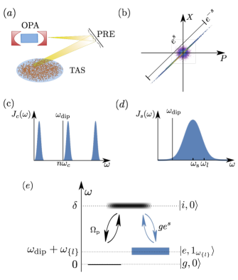
Figure 1: “Color” (a) Experimental setup. The squeezed vacuum is generated via the non-linear processes in the optical parametric amplifier (OPA) operated below threshold. The squeezed vacuum is then reflected by a programmable reflective element (PRE) such as a spatial light modulator (SLM) or a digital mirror device (DMD) and focused to a diffraction limited pattern on the trapped atomic system (TAS). (b) The effect of squeezing in the phase space. Squeezing results in enhanced fluctuations in one quadrature while reducing the fluctuations in the orthogonal quadrature. (c) The spectral density $J_{c}(\omega)$ for a dipole placed within a cavity. The boundary conditions imposed by the cavity mirrors result in a highly modified density of states within the cavity. The change in density of states modifies the $J_{c}(\omega)$ and results in the phenomenology of cQED. (d) The spectral density for a dipole coupled to the anti-squeezed quadrature of the squeezed vacuum beam with a carrier frequency $\omega_{\mathrm{s}}$. The modes within the bandwidth of the squeezed vacuum are labeled by $l\in\{-L,L\}$. (e) A typical application of squeezed vacuum with squeezing parameter $s$ in a stimulated Raman transition that requires a coherent drive with strength $\Omega_{\mathrm{p}}$. The level structure of the quantum degrees of freedom are depicted in the rotating frame of the coherent pump. The labels $g$ and $e$ denote the two metastable qubit states separated by $\omega_{\mathrm{dip}}$ and $i$ denotes the short lived intermediate state whose detuning from the coherent pump is given by $\delta$. All states are shown in a tensor product form (i.e., $|\cdots\rangle\otimes|\cdots\rangle$) with the state of the squeezed electromagnetic modes. The effective coupling strength between the ground and the excited states is $ge^{s}\Omega_{p}/\delta$. We note that the coupling to the dipole operator Eq. (12) is realized when the Raman transition brings the system back to $|g\rangle$, whereas coupling to the operator in Eq. (13) necessitates a balanced Raman scheme.

In the following, we first briefly review the generation of multimode squeezed vacuum in a nonlinear optical cavity. Then, we derive the terms describing the effective dispersive and dissipative interactions mediated by the fluctuations in the squeezed vacuum. We also show how interactions with an arbitrary spatial dependence can be implemented using DMD’s. To assess the experimental feasibility of the squeezed vacuum setup, we estimate the single atom cooperativity that can be achieved using experimentally demonstrated squeezing parameters. Lastly, we discuss some applications of the squeezed vacuum setup in realising exotic quantum phases.

II Squeezed vacuum generation with an optical parametric amplifier

The squeezed vacuum is routinely generated via nonlinear processes in polarizable media Bloembergen1996nonlinear . Here we consider an optical parametric amplifier (OPA) setup where the nonlinear medium is placed inside a high finesse cavity (see Fig. 1 (a)), and pumped by a coherent drive at twice the squeezing frequency $2\omega_{s}$. We assume that the OPA is operated below the oscillation threshold, where the intracavity gain is smaller than the losses, and the output of the non-linear process has a zero mean.

Under these conditions, the creation(annihilation) operator $(\bar{a}^{\dagger}(\bar{a}))$ for the output fields of the OPA satisfies the equation gardiner2004quantum :

$$\bar{a}(\omega) =u(\omega)a_{in}(\omega)-v(\omega)a_{in}^{\dagger}(2\omega_{s}-\omega),$$ (2)

where the operators $a_{in}$ and $a^{\dagger}_{in}$ describe the quantum noise injected into the system from the environment, and ensure that the output operators obey bosonic commutation relations Sachdev1984 ; Carmichael1999statistical . The complex coefficients $u(\omega)$ and $v(\omega)$ obey the bosonic normalisation condition

$$|u(\omega)|^{2}-|v(\omega)|^{2}=1,$$

and describe the squeezing in the output fields. In particular, they define the squeezing parameter $s(\omega)$ by the relation

$$e^{\pm s(\omega)}\equiv|u(\omega)\pm v(\omega)|,$$ (3)

where we have set the squeezing angle to zero (see Appendix A). Then, the fluctuations in the squeezed and anti-squeezed quadratures are scaled by $e^{\pm s(\omega)}$, respectively [see Fig. 1 (b)].

Generically, the frequency bandwidth over which the squeezing degree $s(\omega)$ is non-zero is determined by the lifetime of the intra-cavity photons of the OPA. Recently, anti-squeezing of approximately 20 dB over a 10 MHz bandwidth at optical frequencies has been reported Mehmet2011 ; Vahlbruch2008 . It is important to note that the focus of these experiments was to achieve the largest squeezing possible, which is limited by detection efficiency as much as it is limited by the interaction strength inside the OPA. It is in principle possible to get larger anti-squeezing by driving the OPA closer to the oscillation threshold.

III Atom-field coupling

For the sake of generality, we assume linear coupling between a quadrature $\hat{X}$ of the squeezed vacuum modes and a Hermitian operator $\hat{O}$ describing atomic transitions. In addition, we assume that all the dipole moments are aligned. In the following, we allow the complex amplitudes $\tilde{\Xi}(r)$ of the squeezed vacuum modes to have arbitrary spatial dependencies, since these amplitudes can be shaped using programmable reflective elements as shown in Fig. 1(a).

The model Hamiltonian we use to describe the atom-field system is given by (see Appendix B)

$$H/\hbar =\int d^{2}r(H_{\mathrm{at}}(r)+H^{s}_{\mathrm{vac}}(r)+H_{\mathrm{dip}}(r))/\hbar$$

$$=\int d^{2}rH_{at}(r)/\hbar+\left(\sum_{l}\omega_{l}|\Xi_{l}|^{2}(r)\bar{a}^{\dagger}(\omega_{l})\bar{a}(\omega_{l})+\hat{O}(r)\sum_{l}\eta e^{s(\omega_{l})}\bar{X}_{l}(r)\right),$$ (4)

where $\hat{X}_{l}$ is the squeezed vacuum quadrature given by

$$\bar{X}_{l}(r)=\tilde{\Xi}_{l}(r)\bar{a}(\omega_{l})+(\tilde{\Xi}_{l})^{*}(r)\bar{a}^{\dagger}(2\omega_{s}-\omega_{l}),$$ (5)

with $\tilde{\Xi}_{l}(r)=\Xi_{l}(r)e^{i\varphi_{l}}$ determined by the squeezing transformation. The index $l$ labels the modes within the squeezing bandwidth and $\eta$ is the effective dipole interaction strength, which we assumed to be independent of $l$. The coupling term between the squeezed vacuum quadrature and the atoms arises as a low energy description when the atoms are driven in a Raman scheme Ritsch2013 ; Dimer2007 ; Buchhold2013 . Thus, the time-independent Hamiltonian in Eq. (4) is in the rotating frame that is determined by the frequency $\omega_{\mathrm{p}}$ of the coherent pump. For instance the coupling strength for the scheme in Fig. 1 (e) is $\eta=g\Omega_{\mathrm{p}}/\delta$. Here, $g$ is the bare dipole coupling strength to the electromagnetic vacuum, $\Omega$ is the Rabi frequency due to the coupling to the coherent electromagnetic drive, and $\delta$ is the detuning between the coherent drive frequency and the dipole transition between the ground $|g\rangle$ and the intermediate $|i\rangle$ states. In addition, we emphasize that the quadrature coupling is not essential for the enhancement of interactions. When a Jaynes-Cummings (JC) type interaction is considered, the enhancement of the interaction is simply reduced to half since $a(\omega_{l})=\frac{1}{2}\left(\hat{X}_{l}+\hat{P}_{l}\right)$ (see Appendix D). A simple example of how Eq. (4) can emerge as an effective description of a driven condensate is given in Appendix F.

Figure 2: The Feynman diagram describing the effective interactions between dipoles.

Next, integrating out the squeezed vacuum modes, we obtain pairwise coupling between all pairs of atomic operators $\hat{O}^{\dagger}_{i}\hat{O}_{j}$ for all atoms $i$ and $j$ which spatially overlap with the squeezed vacuum states. The Hermitian part of the effective interaction is given by

$$\tilde{H}_{int} \approx\frac{1}{2}\iint d^{2}rd^{2}r^{\prime}\int d\omega\frac{J(\omega)2\omega}{\omega^{2}_{\mathrm{dip}}-\omega^{2}}\tilde{\Xi}_{\omega}^{*}(r)\tilde{\Xi}_{\omega}(r^{\prime})\hat{O}(r)\hat{O}(r^{\prime})$$

$$=\frac{1}{2}\sum_{l}\iint d^{2}rd^{2}r^{\prime}\tilde{g}_{l}e^{2s(\omega_{l})}\tilde{\Xi}_{l}^{*}(r)\tilde{\Xi}_{l}(r^{\prime})\hat{O}(r)\hat{O}(r^{\prime}),$$ (6)

where $\tilde{g}_{l}\equiv 2\omega_{l}|\eta|^{2}/(\omega^{2}_{\mathrm{dip}}-\omega^{2}_{l})$, and we have used $J(\omega)~{}=~{}\sum_{l}|\eta|^{2}\delta(\omega-\omega_{l})$. We note that to get the above expression, we have projected the interactions to the manifold with no excitation above the squeezed vacuum, ignoring the AC Stark shift terms. The derivation of the effective interaction term using a projector method is given in Appendix C. Derivation of similar terms can be found in Ritsch2013 ; Buchhold2013 ; Douglas2015 ; Strack2011 ; Gopalakrishnan2011 . Because the induced interaction only depends on the spatial overlap between the atoms and the vacuum mode, the interaction Hamiltonian in Eq. (6) describes an infinite-range interaction as long as the vacuum mode is coherent between points $r$ and $r^{\prime}$ (see Appendix C). The coherence length of the squeezed vacuum mode is roughly given by the squeezing bandwidth. When the space-like separation between the dipoles is relevant, relativistic retardation applies to information transfer via such infinite-range interactions.

The anti-Hermitian part of the effective interaction describes the correlated decay processes induced by real photons emitted into the squeezed vacuum. The rate of correlated decay for two particles at $r$ and $r^{\prime}$ is given by the Fermi’s Golden rule

$$\tilde{\gamma}~{}=~{}\frac{2\pi}{\hbar}J_{s}(\overline{\omega})=\frac{2\pi}{\hbar}\sum_{l}\eta^{2}\Xi^{*}_{l}(r)\Xi_{l}(r^{\prime})e^{2s(\omega_{l})}\delta(\bar{\omega}-\omega_{l}),$$ (7)

where $\overline{\omega}$ is the renormalised dipole transition frequency. Besides describing the correlated decay processes into the squeezed vacuum modes, the anti-Hermitian part of the effective interaction can also be used to increase the detection efficiency of light emitted from a single quantum emitter if the decay rate $\tilde{\gamma}$ is comparable to the decay rate into all the other unsqueezed vacuum modes . Moreover, a large cooperativity of the coupling to the squeezed vacuum modes in a traveling-wave geometry entails that an emitter is more likely to emit photons in the propagation direction of the squeezed vacuum beam. In this respect, squeezed vacuum setup provides a natural framework for building chiral networks Lodahl2017 ; Ramos2014 (see Appendix B).

In other words, while the Hermitian part of the effective interaction allows for engineering the Hamiltonian of the atomic system, the anti-Hermitian part allows for engineering the effective reservoir that is responsible for the dissipative dynamics. The dissipative interactions can be implemented between arbitrarily distant dipoles as the strength of dissipative interactions depend not on the squeezing bandwidth, but only on the squeezing parameter at the dipole transition frequency, as long as the squeezing bandwidth is larger than the linewidth of the transition. The situation where the squeezed reservoir results in entanglement between two distant qubits through dissipative dynamics was discussed in Ref. Kraus2004 ; Goldstein1996 ; Banarjee2010 .

We note that the effective interaction between the atomic degrees of freedom can also be calculated in frequency space with the help of the Feynman diagram in Fig. 2. This diagram has the obvious interpretation that the effective interactions between the atomic degrees of freedom are mediated by the dressed photons in the anti-squeezed quadrature. Consequently, what determines the strength and range of the effective dispersive and dissipative interactions are the fluctuations in the electromagnetic vacuum, which are described by dressed photon Green’s function Kulkarni2013 . Using the Green’s function, we show in Appendix C, that the enhanced quadrature fluctuations in a thermal or a Fock state do not lead to an enhancement in the effective coupling, while squeezed number and squeezed thermal states Kim1989 result in the same enhancement as the squeezed vacuum.

Lastly, we discuss how the high tunability of the squeezed vacuum modes can be used to implement translationally invariant finite-range interactions with arbitrary spatial dependence, as well as disordered and time dependent interactions. Because the digital mirror device (DMD) provides a dynamic tuning knob on the spatial profile of the squeezed vacuum modes, it is possible to implement time-averaged Hamiltonians as long as the cycling rate $2\pi\tau_{c}^{-1}$ of the time-periodic Hamiltonian is much faster than the renormalised dynamics of the atomic system. That is, we need

$$|H_{at}|\tau_{c}\ll 1.$$ (8)

The cycling rate should also obey the adiabaticity condition with respect to the energy gap between states with no excitations and a single excitation above the squeezed vacuum. This energy gap can be increased by detuning the atomic transitions further away from the squeezed vacuum, which inevitably reduces the highest achievable effective interaction strength [ see Eq. (6) ] Experimentally, the lower limit of $|H_{at}|$ is determined by the lifetime of the atomic states, whereas the cycling rate can be up to 100 kHz for DMD’s. Remarkably, any translationally invariant interaction potential can be obtained by time-averaging over many speckled vacuum modes goodman2007speckle . If each speckle realisation samples an ensemble characterized by a finite-range spatial autocorrelation function, then the time-averaged Hamiltonian effectively simulates finite range interactions whose spatial dependence is given by the speckle autocorrelation function. That is, the system evolves under an effective time(disorder)-averaged Hamiltonian Haeberlen1968 .

$$\tilde{H}_{\mathrm{int}}^{tav}\approx\sum_{\mathbf{l}}\sum_{i<j}\tilde{g}_{l}e^{2s(\omega_{l})}\overline{\langle\Xi_{l}^{*}(x_{i}-x_{j})\Xi_{l}(0)\rangle}\hat{O}^{\dagger}(x_{i})\hat{O}(x_{j}),$$ (9)

where $\overline{\langle\Xi_{l}^{*}(x_{i}-x_{j})\Xi_{l}(0)\rangle}$ denotes the time(disorder) averaged autocorrelation function. We note that this strategy can be used to implement both dissipative and dispersive finite range interactions The number of disorder samples can be further increased by splitting the squeezed vacuum beam and propagating it over different DMD’s. On the other hand, in the regime where the time-averaging condition is not satisfied, time dependent interactions can be implemented. When only one static speckle pattern is implemented, the Hamiltonian describes disordered interactions.

IV Experimental considerations

The figure of merit for the squeezed vacuum setup is the cooperativity parameter $C$, which is the ratio of the decay rate into the squeezed vacuum modes to the decay rate into all other unsqueezed vacuum modes. Thus, it can be calculated by comparing the spectral densities of the squeezed and unsqueezed vacuum modes at the dipole transition frequency $\overline{\omega}$

$$C=\frac{J_{\mathrm{sq}}(\overline{\omega})}{J(\overline{\omega})} =\frac{\sum^{\prime}_{l}|\eta|^{2}e^{2s(\omega_{l})}\delta(\overline{\omega}-\omega_{l})}{\sum_{l,s}|\eta_{s}|^{2}\delta(\overline{\omega}-\omega_{l})}$$

$$\approx e^{2s(\overline{\omega})}\left(\frac{L^{2}}{A_{\mathrm{foc}}}\right)\frac{\sum^{\prime}_{l}\delta(\overline{\omega}-\omega_{l})}{\sum_{l,s}\delta(\overline{\omega}-\omega_{l})}\equiv C_{0}e^{2s(\overline{\omega})}$$ (10)

where the primed sum goes only over the vacuum modes with non-zero squeezing, $L$ is the linear dimension of space and $A_{\mathrm{foc}}$ is the focal area transverse to the propagation direction of the squeezed vacuum mode. The index $s$ denotes the polarization degree of freedom of the unsqueezed vacuum states. For the second equality, we assumed that the bare dipole coupling stays approximately constant within the squeezing bandwidth around the transition. In the last relation, we defined the cooperativity of unsqueezed modes $C_{0}$. Eq. (10) clearly shows that for the dipole coupling to the squeezed vacuum modes to be significant, the enhancement of fluctuations in the anti-squeezed quadrature should compensate for the reduction of interactions due to the finite solid-angle subtended by the squeezed mode Tanji2011 . When the focal area of the unsqueezed vacuum beam $A_{\mathrm{foc}}$ is decreased down to $\overline{\lambda}^{2}=\left(\frac{\overline{\omega}}{2\pi c}\right)^{2}$, the cooperativity is $C_{0}=\frac{3}{8\pi}\approx 0.1$. Thus, a cooperativity parameter of order 1 can be achieved even with a moderate anti-squeezing degree of 10 dB.

It is also useful to calculate the ratio between the strength of the dispersive interactions to the decay rate. In the weak coupling regime, the ratio is given by the dispersive cooperativity (see Appendix C)

$$C_{\mathrm{disp}}(\omega_{\mathrm{dip}})\approx\left(\frac{L^{2}}{\pi A_{\mathrm{foc}}}\right)\frac{\int d\omega\sum^{\prime}_{l}\frac{2\omega e^{2s(\omega)}}{\omega_{\mathrm{dip}}^{2}-\omega^{2}}\delta(\omega-\omega_{l})}{\sum_{l,s}\delta(\bar{\omega}-\omega_{l})},$$ (11)

where we assumed that the transition frequencies of the dipoles that interact through the squeezed vacuum are identical and given by $\omega_{\mathrm{dip}}$.

In an experimental situation, diffractive losses along the optical path of the squeezed vacuum beam as well as the Lorentzian profile of the squeezing spectrum should be taken into account. While the diffractive losses reduce the cooperativity parameter, the Lorentzian shape of the squeezing spectrum unavoidably reduces the lifetime of the atomic transitions. In Fig. 3, we show $C$ and $C_{\mathrm{disp}}$ as a function of $\delta_{s}=\omega_{s}-\omega_{\mathrm{dip}}$ for an experimental setup where $50\%$ of the squeezed vacuum is lost due to diffraction loudon1983quantum ; Semmler2016 . Moreover, the dipole transition frequency satisfies $\omega_{\mathrm{dip}}\ll\Delta$, such that the rotating-wave approximation is not valid for coupling to the squeezed vacuum modes (see Appendix C). Lastly, we note that by using additional squeezed vacuum beams, the spectral profile of squeezing can also be modified to further increase the dispersive interaction strength.

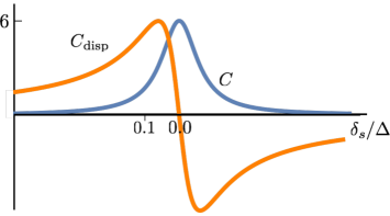
Figure 3: “Color” The single atom cooperativity $C$ and the dispersive cooperativity $C_{\mathrm{disp}}$ as a function of the detuning $\delta_{s}$ between the squeezing and the dipole transition frequencies, normalized by the squeezing bandwidth $\Delta$. The squeezing parameter $s(\omega_{\mathrm{s}})$ is set to give 23 dB squeezing, and 50$\%$ losses is included. Note that the Lorentzian profile of the squeezing spectrum inevitably leads to a enhanced dissipation.

V Applications

We now discuss some of the applications of the squeezed vacuum setup to realise tunable interactions between spin and between density degrees of freedom in artificial quantum many-body systems. We also show how the squeezed vacuum can be used to improve previous experimental proposals for realising exotic orders.

For the implementation of tunable density-density interactions, we identify

$$\hat{O}_{\mathrm{D}}^{\dagger}\equiv\frac{1}{2}(1-\sigma^{\mathrm{z}})\equiv\psi_{g}^{\dagger}\psi_{g},$$ (12)

where $\sigma^{\mathrm{z}}$ is a Pauli matrix which acts on the two dimensional subspace spanned by the ground ($g$) and excited ($e$) states of the atomic system. The resulting coupling has been realised in the recent experiments in cold atom systems Landig2016 . On the other hand, spin-spin interactions can be described by identifying

$$\hat{O}_{\Lambda}^{\dagger}\equiv\sigma^{\mathrm{x}}\equiv\psi_{\uparrow}^{\dagger}\psi_{\downarrow}+\psi_{\downarrow}^{\dagger}\psi_{\uparrow},$$ (13)

where, $\sigma^{\mathrm{x}}$ is a Pauli operator which acts on two nearly degenerate hyperfine levels. An implementation of this coupling in a 4-level atomic systems has been proposed by Ref. Dimer2007 . We note that the above discussion can be extended to atomic systems with more internal degrees of freedom $d$. Here we restrict our attention to $d=1$ and $d=2$ for simplicity.

We emphasize the application of tunable density-density interactions to realize a continuous-space supersolid transition in bosonic systems Prokofiev2012 ; Prokofiev2007 . Briefly, the continuous-space supersolid phase is characterised by the breaking of the continuous spatial translation symmetry and the $U(1)$ phase symmetry of bosonic fields.

The continuous-space supersolid transition in a Bose Einstein condensate can be realised in the squeezed vacuum setup by using multiple squeezed vacuum beams in a traveling wave configuration. To this end, let us consider two traveling squeezed vacuum beams whose spatial profile on the two-dimensional atomic system is given by

$$\Xi_{l}^{\pm}(r)\propto e^{\pm i\mathbf{k}_{0}\cdot r}.$$ (14)

Then, the squeezed vacuum induced interaction between an atom pair $\{i,j\}$ is

$$H_{int}^{ij}(\omega_{l})\propto\cos{[\mathbf{k}_{0}\cdot(\mathbf{r}_{i}-\mathbf{r}_{j})]}\frac{1}{4}(1-\sigma_{z}^{i})(1-\sigma_{z}^{j}).$$ (15)

Thus, the density-density interactions have a characteristic momentum given by $\mathbf{k}_{o}$. If the interaction is attractive, this leads to the softening of the collective modes of the system with momentum $\mathbf{k}_{o}$. When the attractive interactions reach a critical strength the relevant soft modes become unstable, and a density modulation of the condensate with periodicity $\lambda^{-1}_{0}=|\mathbf{k}_{0}|/2\pi$ breaks the continuous translational symmetry of the condensate. In Appendix E, we show that dipole coupling strengths comparable to a recent realisation of a lattice supersolid phase in a cQED setup Landig2016 can be achieved using the squeezed vacuum setup, by using a top-hat spatial profile for the squeezed vacuum beam.

Another application of the squeezed vacuum setup is the realisation of a spin-glass phase by tuning the exchange interactions between localised spins. The Hamiltonian that describes the dispersive interactions between any pair of qubits $(i,j)$ has the form

$$H_{int}(r_{i},r_{j}) \propto\sum_{l}\Xi_{l}^{*}(r_{i})\Xi_{l}(r_{j})\sigma_{i}^{\mathrm{x}}\sigma_{j}^{\mathrm{x}}$$ (16)

By using a static speckle pattern for the spatial profiles $\Xi_{l}$ of the squeezed vacuum beams, it is possible to realize a spin model with disordered interactions. As shown in Ref. Strack2011 ; Buchhold2013 ; Gopalakrishnan2011 , such a model exhibits a spin glass phase as well as ferromagnetic and paramagnetic phases. We also note that a transverse exchange interaction can be implemented when the spins are coupled to the squeezed vacuum through a Jaynes-Cummings (JC) type coupling (see Appendix D). It has been shown that the transverse Heisenberg interaction is sufficient for an implementation of universal quantum computer Imamoglu1999 . For this implementation, as for the cycling rate for the implementation of finite-range interactions, the gate ramp times should be slow enough to avoid transitions into states with non-zero number of excitations on top of the squeezed vacuum state.

VI Conclusion

We propose squeezed vacuum as a valuable resource for engineering dispersive and dissipative interactions in artificial quantum many body systems. We show that experimentally demonstrated values of anti-squeezing gives cooperativity parameters $C>1$. The most important advantage of using squeezed vacuum engineering of the dipole interactions is that the spatial profiles of the electromagnetic vacuum modes can be modified dynamically in a traveling-wave geometry. Thus, the vacuum modes can have an arbitrary profile in the plane perpendicular to the propagation direction. Using this dynamical control, we showed how to implement arbitrary finite range interaction potentials in a time-averaged fashion.

We would like to emphasize that the idea of using the squeezed vacuum to engineer interactions between dipoles is platform independent. Thus, it can be used to deterministically generate entanglement between any two atomic dipoles whether they are implemented via quantum dots, NV centers Wrachtrup2006 , or real atoms, opening up new possibilities for hybrid systems. One exciting observation is that the entangling interactions can be implemented in macroscopic length scales as long as the distance between the dipoles is shorter than the coherence length of the squeezed vacuum, which is determined by the squeezing bandwidth. Lastly, the enhanced fluctuations in the squeezed electromagnetic vacuum can be transferred to other vacuum fluctuations such as phonons in crystals or condensates. Thus, one can enhance the interactions between these phonons and other electronic degrees of freedom Cotlet2016 ; Knap2016 .

Appendix A Squeezing spectrum

In this Appendix, we follow the standard derivation of the squeezing properties of the output field from an OPA gardiner2004quantum .

A.0.1 The equations of motion in frequency space

Two mode squeezed light can be generated using parametric down conversion. Consider the Hamiltonian in the rotating frame of the pump frequency

$$H_{PDC}=\hbar\omega_{0}(a^{\dagger}a+b^{\dagger}b)+i\hbar\left(\epsilon a^{\dagger}b^{\dagger}e^{-i\omega_{p}t}-\epsilon^{*}abe^{+i\omega_{p}t}\right),$$ (17)

where $\omega_{p}$ is the OPA pump frequency and $\omega_{0}$ is the frequency of the OPA cavity modes. We write down the Heisenberg-Langevin equations of motion for the cavity modes using $\frac{\partial A}{\partial t}=\frac{i}{\hbar}[H,A]$

$$\dot{a}(t) =-i\omega_{0}a(t)+\epsilon b^{\dagger}(t)e^{-i\omega_{p}t}-\frac{\gamma_{1}}{2}a(t)-\sqrt{\gamma_{1}}a_{in}(t)$$ (18)

$$\dot{b}(t) =-i\omega_{0}b(t)+\epsilon a^{\dagger}(t)e^{-i\omega_{p}t}-\frac{\gamma_{1}}{2}b(t)-\sqrt{\gamma_{1}}b_{in}(t),$$ (19)

where $a_{in}$ and $b_{in}$ are the input noise operators for the corresponding cavity modes, and we assumed that the cavity where the $\chi^{2}$ material is in has only one decay channel with rate $\gamma_{1}$.

We can solve this equation by going to the fourier domain

$$a(t)=\frac{1}{\sqrt{2\pi}}\int d\omega e^{-i\omega t}a(\omega)$$ (20)

$$[a(t)]^{\dagger}=a^{\dagger}(t)=\frac{1}{\sqrt{2\pi}}\int d\omega e^{i\omega t}a^{\dagger}(\omega),$$ (21)

and the same for $b$. Specifically,

$$\int dt\,b^{\dagger}(t)e^{i(\omega-\omega_{p})t}=b^{\dagger}(\omega_{p}-\omega).$$ (22)

Then, taking the Fourier transform of the equation of motion, we get

$$i(\omega_{p}-\omega)a^{\dagger}(\omega_{p}-\omega)=$$

$$+i\omega_{0}a^{\dagger}(\omega_{p}-\omega)+\epsilon^{*}b(\omega)-\frac{\gamma_{1}}{2}a^{\dagger}(\omega_{p}-\omega)-\sqrt{\gamma_{1}}a_{in}^{\dagger}(\omega_{p}-\omega)$$

$$i(\omega_{p}-\omega)b^{\dagger}(\omega_{p}-\omega)=$$

$$+i\omega_{0}b^{\dagger}(\omega_{p}-\omega)+\epsilon^{*}a(\omega)-\frac{\gamma_{1}}{2}b^{\dagger}(\omega_{p}-\omega)-\sqrt{\gamma_{1}}b_{in}^{\dagger}(\omega_{p}-\omega)$$

$$-i\omega a(\omega)=-i\omega_{0}a(\omega)+\epsilon b^{\dagger}(\omega_{p}-\omega)-\frac{\gamma_{1}}{2}a(\omega)-\sqrt{\gamma_{1}}a_{in}(\omega)$$

$$-i\omega b(\omega)=-i\omega_{0}b(\omega)+\epsilon a^{\dagger}(\omega_{p}-\omega)-\frac{\gamma_{1}}{2}b(\omega)-\sqrt{\gamma_{1}}b_{in}(\omega)$$ (23)

Now setting $\omega_{p}=2\omega_{0}\,\dot{=}\,2\omega_{s}$ we can write the following set of linear equations as

$$\mathbf{a}(\omega)=\left(A-\left(\frac{\gamma_{1}}{2}-i(\omega-\omega_{s})\right)\right)^{-1}\sqrt{\gamma_{1}}\mathbf{a}_{in}(\omega),$$ (25)

where

$$\mathbf{a}(\omega)=\left(\begin{array}[]{c}a(\omega)\\ b(\omega)\\ a^{\dagger}(2\omega_{s}-\omega)\\ b^{\dagger}(2\omega_{s}-\omega)\end{array}\right)\quad\mathrm{and}\quad A=\left(\begin{array}[]{cccc}0&0&0&\epsilon\\ 0&0&\epsilon&0\\ 0&\epsilon^{*}&0&0\\ \epsilon^{*}&0&0&0\end{array}\right).$$ (34)

The inverse of this matrix we need is

$$\left(A-\left(\frac{\gamma_{1}}{2}-i(\omega-\omega_{s})\right)\right)^{-1}=\frac{1}{(\frac{\gamma_{1}}{2}-i(\omega-\omega_{s}))^{2}-|\epsilon|^{2}}\times$$

$$\left(\begin{array}[]{cccc}-(\frac{\gamma_{1}}{2}-i(\omega-\omega_{s}))&0&0&-\epsilon\\ 0&-(\frac{\gamma_{1}}{2}-i(\omega-\omega_{s}))&-\epsilon&0\\ 0&-\epsilon^{*}&-(\frac{\gamma_{1}}{2}-i(\omega-\omega_{s}))&0\\ -\epsilon^{*}&0&0&-(\frac{\gamma_{1}}{2}-i(\omega-\omega_{s}))\end{array}\right),$$ (39)

The intracavity fields can be written as

$$a(\omega) =\tilde{u}(\omega)a_{in}(\omega)-\tilde{v}(\omega)b_{in}^{\dagger}(2\omega_{s}-\omega)$$ (40)

$$b(\omega) =\tilde{u}(\omega)b_{in}(\omega)-\tilde{v}(\omega)a_{in}^{\dagger}(2\omega_{s}-\omega)$$ (41)

where we defined

$$\tilde{u}(\omega)=-\frac{(\frac{\gamma_{1}}{2}-i(\omega-\omega_{s}))\sqrt{\gamma_{1}}}{(\frac{\gamma_{1}}{2}-i(\omega-\omega_{s}))^{2}-|\epsilon|^{2}}$$ (42)

$$\tilde{v}(\omega)=\frac{\epsilon\sqrt{\gamma_{1}}}{(\frac{\gamma_{1}}{2}-i(\omega-\omega_{s}))^{2}-|\epsilon|^{2}}.$$ (43)

Using this, we note the important symmetry of these so called coherence factors.

$$\tilde{u}(\omega) =\tilde{u}^{*}(2\omega_{s}-\omega)$$ (44)

$$\tilde{v}(\omega) =e^{i2\vartheta_{s}}\tilde{v}^{*}(2\omega_{s}-\omega),$$ (45)

where we defined the squeezing angle $\vartheta_{s}$. The above relations reflect the energy conservation law for the squeezed excitation. That is, the excitations on top of the squeezed vacuum are a superposition of one photon excitation with frequency ($\omega_{1}$) and one photon hole with frequency ($\omega_{2}$) with the constraint

$$\omega_{1}+\omega_{2}=2\omega_{s}=\omega_{p}.$$ (46)

The phase information in the imaginary part in the denominator simply reflects the $\pi$ shift over the resonance for $\tilde{u}(\omega)$, whereas $\tilde{v}(\omega)$ also includes the squeezing angle information. For a single sided cavity, the squeezing angle is independent of $\omega$.

A.0.2 The output field of the OPA

We are interested in the output field of the parametric down converter. This is obtained using the input-output relation, which reads

$$a_{out}(\omega) \equiv\bar{a}(\omega)=a_{in}(\omega)+\sqrt{\gamma_{1}}a(\omega)$$

$$=u(\omega)a_{in}(\omega)-v(\omega)b_{in}^{\dagger}(2\omega_{s}-\omega).$$ (47)

where $u$, $v$ are

$$u(\omega) =1+\sqrt{\gamma_{1}}\tilde{u}(\omega)=1-\frac{(\frac{\gamma_{1}}{2}-i(\omega-\omega_{s}))\gamma_{1}}{(\frac{\gamma_{1}}{2}-i(\omega-\omega_{s}))^{2}-|\epsilon|^{2}}$$

$$=-\frac{(\frac{\gamma_{1}}{2})^{2}+(\omega-\omega_{s})^{2}+|\epsilon|^{2}}{(\frac{\gamma_{1}}{2}-i(\omega-\omega_{s}))^{2}-|\epsilon|^{2}}$$ (48)

$$v(\omega) =\sqrt{\gamma_{1}}\tilde{v}(\omega)=\frac{\gamma_{1}\epsilon}{\left(\gamma_{1}/2-i(\omega-\omega_{s})\right)^{2}-|\epsilon|^{2}}$$ (49)

Note that the symmetries in Eq. (45) are preserved, and now

$$|u(\omega)|^{2}-|v(\omega)|^{2}=1.$$

As a result, we simply obtain a squeezed vacuum in terms of the input noise fields. Also note that the large squeezing limit happens when $\epsilon$ approaches $\gamma/2$ from below. In this limit $|u(\omega)|\approx|v(\omega)|$. Also note that the normalisation ensures that the inverse transform reads

$$a_{in}(\omega)=u(\omega)\bar{a}(\omega)+v(\omega)\bar{b}^{\dagger}(2\omega_{s}-\omega),$$ (50)

In order to take into account the diffractive losses we need to use the following expression for the output field loudon1983quantum .

$$\bar{a}=\sqrt{\epsilon_{\mathrm{diff}}}\left(a_{\mathrm{in}}(\omega)+\sqrt{\gamma_{1}}a(\omega)\right)+\sqrt{1-\epsilon_{\mathrm{diff}}}c(\omega),$$ (51)

where $c(\omega)$ represent the noise that is injected into the squeezed vacuum due to losses, and $\epsilon_{\mathrm{diff}}$ is the power loss due to diffraction. It has the noise properties of unsqueezed vacuum and obeys

$$[a(\omega),c(\omega^{\prime})]=[a_{\mathrm{in}}(\omega),c(\omega^{\prime})]=0.$$ (52)

The type of noise injected into the squeezed vacuum due to losses can be specified by specifying the correlation functions for $c(\omega)$. This completes our discussion of the generation of squeezed vacuum using an OPA.

Appendix B Coupling to squeezed vacuum source

In this Appendix, we derive the interaction Hamiltonian in Eq. 4 between the squeezed vacuum generated by an OPA and an atom which overlaps with the output of the OPA. To this end, we follow the work of Gardiner Gardiner1993 and Carmichael Carmichael1993 on cascaded quantum systems.

The Hamiltonian that we are interested in is

$$H/\hbar =H_{sys}/\hbar+\int dl\omega_{l}b_{l}^{\dagger}b_{l}+\int dl\kappa_{c}(l)(ab_{l}^{\dagger}+h.c.)$$

$$+\int d_{l}\kappa_{a}(l)(\sigma^{-}b_{l}^{\dagger}e^{-i\omega_{l}\tau}+h.c.),$$ (53)

where $l$ labels the vacuum modes that serve as the common bath modes for the OPA cavity and the atom, whose creation(annihilation) operators are given by $a^{\dagger}(a)$ and $\sigma^{+}(\sigma^{-})$, respectively. The coupling constants $\kappa_{a}$ and $\kappa_{c}$ depend on $l$ in general. The extra phase factor, $e^{-i\omega_{l}\tau}$ on the atom-field coupling is due to the distance between the source and the atom. For simplicity, we have not considered the quadrature coupling in this section, but the generalization is immediate.

Assuming now that the coupling of the cavity to the electromagnetic field modes is Markovian [i.e., $\kappa_{c}(l)\equiv\sqrt{\gamma_{1}}$], the equation of motion for the electromagnetic field has the solution

$$b(l,t)=e^{-i\omega_{l}(t-t_{0})}b(l,t_{0})$$

$$+\int_{t_{0}}^{t}dt^{\prime}e^{-i\omega_{l}(t-t^{\prime})}\left[\sqrt{\gamma_{1}}a(t^{\prime})+\tilde{\kappa}_{a}(l)\sigma^{-}(t^{\prime})\right],$$ (54)

where $\tilde{\kappa}_{a}(l)\equiv\kappa_{a}(l)e^{-i\omega_{l}\tau}$. On the other hand, the equation of motion of the atomic degree of freedom is given by

$$\dot{\sigma}^{-}(t)=-i\omega_{\mathrm{at}}\sigma^{-}(t)-i\int dl\tilde{\kappa}_{a}(l)b(l,t),$$ (55)

with the atomic transition frequency $\omega_{\mathrm{at}}$. Plugging in the solution for the electromagnetic field, one obtains

$$\dot{\sigma}^{-}(t)=-i\omega_{at}\sigma^{-}(t)-i\int dl\tilde{\kappa}_{a}(l)\bigg{\{}e^{-i\omega_{l}(t-t_{0})}b(l,t_{0})$$

$$+\int_{t_{0}}^{t}dt^{\prime}e^{-i\omega_{l}(t-t^{\prime})}\left[\sqrt{\gamma_{1}}a(t^{\prime})+\tilde{\kappa}_{a}(l)\sigma^{-}(t^{\prime})\right]\bigg{\}},$$ (56)

whose fourier transform is

$$i(\omega-\omega_{\mathrm{at}})\sigma^{-}(\omega)=i\int_{t_{0}}^{\infty}dt\bigg{(}\int dl\tilde{\kappa}_{a}(l)\bigg{\{}e^{i\omega t}e^{-i\omega_{l}(t-t_{0})}b(l,t_{0})$$

$$+\int_{t_{0}}^{t}dt^{\prime}e^{i\omega t}e^{-i\omega_{l}(t-t^{\prime})}\left[\sqrt{\gamma_{1}}a(t^{\prime})+\tilde{\kappa}_{a}(l)\sigma^{-}(t^{\prime})\right]\bigg{\}}\bigg{)},$$ (57)

The first term in the right hand side can be related to the $l$ components of the noise operator,

$$\int dl\tilde{\kappa}_{a}(l)e^{i\omega_{l}t_{0}}b(l,t_{0})\delta(\omega-\omega_{l})\equiv\int dl\tilde{\kappa}_{a}(l)a_{in}(l)\delta(\omega-\omega_{l}),$$ (58)

which couples only at frequency $\omega_{l}$. To evaluate the second term, we need a couple of assumptions. Re-arranging and setting $t_{0}=0$, we have

$$\int dl\sqrt{\gamma_{1}}\tilde{\kappa}_{a}(l)\int_{0}^{\infty}dte^{i(\omega-\omega_{l})t}\int_{0}^{t}dt^{\prime}e^{i\omega_{l}t^{\prime}}a(t^{\prime}),$$ (59)

the rightmost integral is evaluated by plugging in the fourier expansion of $a(t^{\prime})=\int_{-\infty}^{\infty}d\omega^{\prime}\exp{(-i\omega^{\prime}t^{\prime})}a(\omega^{\prime})$

$$\int_{0}^{t}dt^{\prime}e^{i\omega_{l}t^{\prime}}a(t^{\prime}) =\int_{-\infty}^{\infty}d\omega^{\prime}a(\omega^{\prime})\int_{0}^{t}dt^{\prime}e^{i(\omega_{l}-\omega^{\prime})t^{\prime}}$$

$$=\int_{-\infty}^{\infty}d\omega^{\prime}a(\omega^{\prime})\int_{-\infty}^{\infty}dt^{\prime}e^{i(\omega_{l}-\omega^{\prime})t^{\prime}}\mathrm{Sq}(0,t),$$ (60)

where $\mathrm{Sq}(0,t)$ is a square function from $0$ to $t$. Note that $t$ gives us the time scale where we would like to describe the dynamics of the dipole in question. In steady state, we can take $t$ as far from $0$ as we want. Correspondingly, in steady state, we obtain

$$\int_{-\infty}^{\infty}d\omega^{\prime}a(\omega^{\prime})\int_{-\infty}^{\infty}dt^{\prime}e^{i(\omega_{l}-\omega^{\prime})t^{\prime}}\mathrm{Sq}(0,t)$$

$$\approx\int_{-\infty}^{\infty}d\omega^{\prime}a(\omega^{\prime})\delta(\omega_{l}-\omega^{\prime})=a(\omega_{l}),$$ (61)

where the $\delta$ function actually has the width of $2\pi/t$. The second integral over $t$ gives an additional factor of $\delta(\omega_{l}~{}-~{}\omega)$. Thus, the electromagnetic vacuum couples to the dynamics in an energy-conserving way. As a result, we obtain,

$$-i\omega\sigma^{-}(\omega) =-i\omega_{at}\sigma^{-}(\omega)-i\int dl\tilde{\kappa}_{a}(l)\left[a_{in}(l)+\sqrt{\gamma_{1}}a(\omega_{l})\right]$$

$$=-i\omega_{at}\sigma^{-}(\omega)-i\int dl\tilde{\kappa}_{a}(l)a_{\mathrm{out}}(\omega_{l}),$$ (62)

where $a_{\mathrm{out}}$ is defined as in Eq. (47), and we have included in the renormalized transition frequency $\tilde{\omega}_{at}~{}=~{}\omega_{at}+\Delta_{\mathrm{Lamb}}-i\gamma_{at}$, the Lamb shift $\Delta_{\mathrm{Lamb}}$ and spontaneous decay rate $\gamma_{at}$ of the atomic transition due to its coupling to the free electromagnetic modes. The interaction Hamiltonian that produces this equation of motion is

$$H_{I}^{eff}/\hbar=\int dl\tilde{\kappa}_{a}(l)a_{\mathrm{out}}(\omega_{l})\sigma^{+}+h.c.\,.$$ (63)

Notice the above equation is what we have used in the main text when the diffractive losses replace $a_{out}\rightarrow\bar{a}$ as in Eq. (51).

In the cascaded system the chirality of the interactions, that is , the fact that the OPA field can influence the atom without being influenced by the atom, can be seen by restricting the $l$ summation over the modes to ones whose wavevectors satisfy $k_{l}\cdot{(r_{\sigma}-r_{a})}>0$, where $r_{\sigma}-r_{a}$ is the displacement vector from the cavity and the atom. For simplicity, let us consider the one dimensional situation where we consider the bath modes $b_{l}$ which are plane waves whose wavenumber $k_{l}$ is aligned with $(r_{\sigma}~{}-~{}r_{a})=c\tau\hat{x}$ with $c\tau>0$. Then, defining the spatial fourier transform of the common bath modes $b(l,t)$ as

$$b(x,t)=\int dlb(l,t)e^{i\omega_{l}/cx},$$ (64)

where $x$ is measured with respect to the cavity, we find that the contribution of the OPA to $b(r,t)$ is

$$b(x,t)\bigg{|}_{a} =\int_{t_{0}}^{t}dt^{\prime}\Theta(t-t^{\prime})\int dle^{i\omega_{l}(x/c-t+t^{\prime})}\sqrt{\gamma_{1}}a(t^{\prime})$$

$$=\Theta(x/c)\sqrt{\gamma_{1}}a(t-x/c),$$ (65)

where the contribution with $x\rightarrow-x$ is absent because of the restriction $k_{l}>0$. Thus, the influence of the cavity is only to the systems that are to its right.

Similarly, the influence of the atom also propagates to the right since the contribution to the bath modes is

$$b(x,t)\bigg{|}_{\sigma}=\int_{t_{0}}^{t} dt^{\prime}\Theta(t-t^{\prime})\sigma^{-}(t^{\prime})\tilde{\kappa}_{a}(t-t^{\prime}-x/c+\tau),$$ (66)

where $\tilde{\kappa}_{a}(x)\equiv\int dle^{i\omega_{l}x}\kappa_{a}(l)$. We note that the contribution of the off-resonant atom is non-Markovian. To recover the Markovian expression, we replace $\kappa_{a}(l)$ by $\sqrt{\gamma_{a}}$, and $\tilde{\kappa}_{a}(t-t^{\prime}-x/c+\tau)$ by $\delta(t-t^{\prime}-x/c+\tau)$, to obtain familiar contribution loudon1983quantum

$$b(x,t)\bigg{|}_{\sigma}=\Theta(x/c-\tau)\sqrt{\gamma_{a}}\sigma^{-}(t-x/c+\tau).$$ (67)

For a more non-trivial case of the coupling function $\kappa_{a}(l)$, let us consider $\kappa_{a}(l)\equiv\frac{\gamma}{\gamma^{2}+(\omega_{s}-\omega_{l})^{2}}$, where $\omega_{s}$, and $\gamma$ can be thought of as the carrier frequency and the bandwidth of the squeezed vacuum, respectively. Then the contribution of the atom to the common bath mode can be calculated using the residue theorem.

$$b(x,t)\bigg{|}_{\sigma} \propto$$

$$\int_{t_{0}}^{t}dt^{\prime}\bigg{\{}\Theta(t-t^{\prime})\sigma^{-}(t^{\prime})e^{-(\gamma-i\omega_{s})|t-t^{\prime}-x/c+\tau|}\bigg{\}}.$$

Now let us look at the field distribution around the position of the atom. With $\delta x\equiv x-c\tau$, $\delta t\equiv t-t^{\prime}$, and a shift of the time integral to the integration variable $\bar{t}\equiv\delta t-\delta x$, we get ($c\equiv 1$)

$$b(x,t)\bigg{|}_{\sigma} \propto\int^{t-t_{0}-\delta x}_{-\delta x}d\bar{t}\Theta(\delta x+\bar{t})\sigma^{-}(t-\bar{t}-\delta x)e^{-(\gamma-i\omega_{s})|\bar{t}|},$$ (68)

Unlike the Markovian case, the atomic contribution to the bath mode at time $t$ and $x$ is non-vanishing for $|\delta x|~{}>~{}0$ although the bath modes that couple to the atom have a definite chirality. However, as expected, the influence of the atom extends more to the right ($\delta x>0$) than to the left ($\delta x<0$), due to the exponential factor in the integrand.

Lastly, we note that in the main text, we incorporated the free evolution of the output field of the OPA by $\hbar\int dl\omega_{l}a^{\dagger}_{\mathrm{out}}(l)a_{\mathrm{out}}(l)$, which holds thanks to the energy conservation in the steady state which enabled us to employ delta functions above.

Appendix C Green’s functions

Here we give a brief introduction to the Green’s function methods cohen1992atom to describe the effective dynamics of the atomic system placed within the squeezed vacuum. We project the many-body Schroedinger equation onto the manifold of atomic and the squeezed vacuum states that are of interest. Then we derive the effective Hamiltonian for these atomic states in the pole approximation. The effective interactions between dipoles placed in the squeezing vacuum can be described by the so called level shift operator projected onto the subspace $\{\alpha\}$ of the many body atomic states tensored with the squeezed vacuum state in the suitable rotating frame. We note that the derivation of the effective Hamiltonian using the Green’s function methods does not rely on a rotating-wave approximation.

To this end, we define the projection operator onto $\{\alpha\}$

$$P_{\{\alpha\}} =\sum_{i\in\{\alpha\}}|i\rangle\langle i|$$ (69)

$$Q_{\{\alpha\}} =\mathbf{I}-P_{\{\alpha\}}=\sum_{i\not\in\{\alpha\}}|i\rangle\langle i|.$$ (70)

The projector operators obey $P^{2}_{\{\alpha\}}=P_{\{\alpha\}}$, $Q^{2}_{\{\alpha\}}=Q_{\{\alpha\}}$, and $Q_{\{\alpha\}}P_{\{\alpha\}}=0$. Moreover, $P_{\{\alpha\}}H_{0}Q_{\{\alpha\}}=0$.

Now, the Green’s function operator is defined as

$$(z-H)G(z)=(z-H_{0}-V)G(z)=\mathbf{I},$$ (71)

where $z\in\mathbf{C}$. Multiplying the above equation by $P_{\{\alpha\}}$ from the right, we obtain

$$(z-H_{0}-V)(P^{2}_{\{\alpha\}}+Q^{2}_{\{\alpha\}})G(z)P_{\{\alpha\}}=P_{\{\alpha\}}.$$ (72)

Then multiplying the above equation on the left with $Q_{\{\alpha\}}$ and using the properties of the projector operators that are mentioned above, we obtain

$$Q_{\{\alpha\}}G(z)P_{\{\alpha\}}=\frac{Q_{\{\alpha\}}VP_{\{\alpha\}}}{Q_{\{\alpha\}}(z-H)Q_{\{\alpha\}}}(P_{\{\alpha\}}G(z)P_{\{\alpha\}}).$$ (73)

On the other hand, multiplying Eq. (72) on the left with $P_{\{\alpha\}}$ and substituting in Eq. 73 , we find that the projected Greens function operator satisfies the following equation

$$P_{\{\alpha\}}\left[z-H-V\frac{Q_{\{\alpha\}}}{Q_{\{\alpha\}}(z-H)Q_{\{\alpha\}}}V\right]P_{\{\alpha\}}G(z)P_{\{\alpha\}}=P_{\{\alpha\}}.$$ (74)

Thus, the projected Green’s function operator has the form

$$G_{\{\alpha\}}(z)\equiv P_{\{\alpha\}}G(z)P_{\{\alpha\}}=\frac{P_{\{\alpha\}}}{P_{\{\alpha\}}(z-H_{0}-R(z))P_{\{\alpha\}}},$$ (75)

where

$$R(z)=V+V\frac{Q_{\{\alpha\}}}{Q_{\{\alpha\}}(z-H)Q_{\{\alpha\}}}V,$$ (76)

is called the level-shift, or the self-energy operator. The level-shift operator can be expanded in powers of the interaction Hamiltonian $V$

$$R(z) =V+V\frac{Q_{\{\alpha\}}}{z-Q_{\{\alpha\}}H_{0}Q_{\{\alpha\}}}V$$

$$+V\frac{Q_{\{\alpha\}}}{z-Q_{\{\alpha\}}H_{0}Q_{\{\alpha\}}}V\frac{Q_{\{\alpha\}}}{z-Q_{\{\alpha\}}H_{0}Q_{\{\alpha\}}}V+\cdots.$$ (77)

So far, we have kept the discussion very general. However, the level - shift operator is greatly simplified when the interaction Hamiltonian only couples the bath and atomic degrees of freedom such that the terms proportional to $Q_{\{\alpha\}}VQ_{\{\alpha\}}$ vanish. This results in

$$R(z)=V+V\frac{Q_{\{\alpha\}}}{z-Q_{\{\alpha\}}H_{0}Q_{\{\alpha\}}}V.$$ (78)

The real and the imaginary parts of the shift operator are found using the Sokhotski-Plemelj identity

$$\frac{1}{x\pm i0^{+}}=\mathcal{P}\frac{1}{x}\mp i\pi\delta(x),$$ (79)

where $\mathcal{P}$ denotes the principle value. Then, near the real number line the Hermitian and the anti-Hermitian parts of the shift operator are given by

$$R(E\pm i0^{+}) =V+\mathcal{P}V\frac{Q_{\{\alpha\}}}{Q_{\{\alpha\}}(E\pm i0^{+}-H_{0})Q_{\{\alpha\}}}V$$

$$\mp i\pi VQ_{\{\alpha\}}\delta(E-Q_{\{\alpha\}}H_{0}Q_{\{\alpha\}})Q_{\{\alpha\}}V$$

$$=V+\Sigma(E\pm i0^{+})\mp i\hbar\Gamma(E)/2.$$ (80)

It is clear that the shift operator changes the energy levels and introduces decay rates inside the projected state space $\{\alpha\}$ due to the interactions with the states outside of $\{\alpha\}$. If the Hermitian part of the shift operator is small compared to the bare energies $\{E_{\alpha}\}$ of the states in $\{\alpha\}$, one can apply the so called pole approximation to arrive at the approximation of the Green’s function

$$G_{\{\alpha\}}(E\pm i0^{+}) \approx\frac{P_{\{\alpha\}}}{P_{\{\alpha\}}(E-H_{0}-V-\Sigma(\{E_{\alpha}\})\mp i(\frac{\hbar}{2}\Gamma(\{E_{\alpha}\})+0^{+}))P_{\{\alpha\}}}\equiv\frac{P_{\{\alpha\}}}{P_{\{\alpha\}}(E-H_{\{\alpha\}}+i0^{+})P_{\{\alpha\}}},$$ (81)

where we defined the projected Hamiltonian

$$H_{\{\alpha\}}(\{E_{\alpha}\})=H_{0}+V+\Sigma(\{E_{\alpha}\})+i\frac{\hbar}{2}\Gamma(\{E_{\alpha}\}).$$ (82)

In the above equations, expressions $\Sigma(\{E_{\alpha}\})$ and $\Gamma(\{E_{\alpha}\})$ take $E_{\alpha}$ as their arguments depending on the specific state $\alpha$ that $P_{\{\alpha\}}$ projects the interaction term onto.

The matrix elements of the effective Hamiltonian can now be calculated. As mentioned in the main text, we are interested in the interactions that are within the zero photon manifold. For instance the matrix element associated to the exchange of an excitation between two dipoles with transition frequency $\omega_{\mathrm{dip}}$ is given by

$$\langle g,e;\{0_{l}\}|\Sigma(\omega_{\mathrm{dip}})|e,g,;\{0_{l}\}\rangle$$

$$=\langle g,e;\{0_{l}\}|V\frac{1}{\omega_{dip}-H_{0}}V|e,g,;\{0_{l}\}\rangle$$

$$=\sum_{l}g_{l}(r_{1})g_{l}(r_{2})\left(\frac{1}{\omega_{\mathrm{dip}}-\omega_{l}}+\frac{1}{\omega_{\mathrm{dip}}-(\omega_{l}+2\omega_{\mathrm{dip}})}\right)$$

$$=\sum_{l}g_{l}(r_{1})g_{l}(r_{2})\frac{2\omega_{l}}{\omega_{\mathrm{dip}}^{2}-\omega_{l}^{2}},$$ (83)

where the intermediate two-qubit states in the one photon manifold have energies $H_{0}|g,g;1_{l}\rangle=\omega_{l}$ and $H_{0}|e,e;1_{l}\rangle=(\omega_{l}+2\omega_{\mathrm{dip}})|e,e;1_{l}\rangle$. We also assumed that dipolar coupling strength $g_{l}$ at positions $r_{1}$ and $r_{2}$ are real for simplicity. We took the interaction potential between the bath and the two dipoles to be of the form $V~{}=~{}\sum_{l}\left(g_{l}(r_{1})\sigma_{1}^{+}X_{l}+g_{l}(r_{2})\sigma_{2}^{+}X_{l}\right)$.

Using the above procedure, it is also easy to show that a thermal state, or a Fock state of photons does not increase the effective coupling strength. To this end, consider an initial state where each electromagnetic mode $l$ is in a Fock state with $n_{l}$ photons, the intermediate states that need to be taken into account are: $|e,e;\{n_{l};n_{l^{\prime}}+1\}\rangle$, $|e,e;\{n_{l};n_{l^{\prime}}-1\}\rangle$, $|g,g;\{n_{l};n_{l^{\prime}}+1\}\rangle$, $|g;g;\{n_{l};n_{l^{\prime}}-1\}\rangle$. Here we used the following notation

$$|g;g;\{n_{l};n_{l^{\prime}}-1\}\rangle=|g\rangle\otimes|g\rangle\otimes|n_{1},n_{2},\cdots,n_{l^{\prime}}-1,\cdots\rangle.$$ (84)

These states have the bare energies $H_{0}|g,e;\{n_{l}\}\rangle\equiv H_{0}|e,g;\{n_{l}\}\rangle=\omega_{\mathrm{dip}}+\sum_{l}n_{l}\omega_{l}$. Thus, the matrix element of $\Sigma(\omega_{\mathrm{dip}})$ becomes

$$\langle g,e;\{n_{l}\}|\Sigma\left(\omega_{\mathrm{dip}}+\sum_{l}\omega_{l}n_{l}\right)|e,g,;\{n_{l}\}\rangle$$

$$=\sum_{l}(n_{l}+1)g_{l}^{2}\left[\frac{1}{\omega_{\mathrm{dip}}-\omega_{l}}+\frac{1}{\omega_{\mathrm{dip}}-\omega_{l}-2\omega_{\mathrm{dip}}}\right]$$

$$-(n_{l})g_{l}^{2}\left[\frac{1}{\omega_{\mathrm{dip}}-\omega_{l}}+\frac{1}{\omega_{\mathrm{dip}}-\omega_{l}-2\omega_{\mathrm{dip}}}\right]$$

$$=\sum_{l}g_{l}^{2}\frac{2\omega_{l}}{\omega_{\mathrm{dip}}^{2}-\omega_{l}^{2}},$$

and we observe that the strength of the effective interactions does not depend on $\{n_{l}\}$. Yet, the strength of the interaction mediated by squeezed Fock or thermal states is still enhanced since then we should replace $g_{l}\rightarrow g_{l}e^{s(\omega_{l})}$. We emphasize that the above procedure does not assume rotating-wave or Markov approximations.

On the other hand, the decay rate is concerned with a transition between two states with different photon numbers. If we consider the quantity $|\langle e,0|G(E+i0^{+})|e,0\rangle|^{2}$, and transform the expression back into the time domain, we obtain the decay rate of the population to be

$$\Gamma(\omega_{\mathrm{dip}})=\frac{2\pi}{\hbar}\sum_{l}g_{l}^{2}\delta(\omega_{l}-\omega_{\mathrm{dip}}).$$ (85)

The cooperativity $C$ and dispersive cooperativity $C_{\mathrm{disp}}$ were calculated by comparing the self-energies induced by the squeezed vacuum focused on the atoms to the imaginary part of the self energy induced by the coupling of the atom to the unsqueezed vacuum modes.

Lastly, we would like to note that although we have assumed the pole approximation here, the problem of a single emitter coupled to a squeezed vacuum quadrature is indeed exactly solvable without the rotating-wave or Markov approximations cohen1992atom . Here our focus has been on the potential of squeezed vacuum states, and not the solution to a specific problem.

To summarise, we briefly introduced the Green’s function framework to describe the effective dynamics of the atomic degrees of freedom in the presence of a squeezed vacuum.

Appendix D Quadrature vs. Jaynes-Cummings Hamiltonians

In this Appendix, we extend our analysis of the quadrature coupling between the dipole transitions and the vacuum modes to a Jaynes-Cummings type interaction where the contribution of anti-resonant terms are ignored. We show that in the simplest case of a single squeezed mode, the enhancement factor is reduced by half, as the dipole transition couples to both the squeezed and anti-squeezed vacuum fluctuations.

For the Dicke model, the coupling of the atomic dipole is to the quadrature of the vacuum mode. Then the action of squeezing transformation on the quadrature operator is

$$\bar{X}(r) =\sum_{l}U^{\dagger}_{l}X_{l}(r)U_{l}=\sum_{l}U^{\dagger}_{l}\frac{\Xi_{l}(r)}{2}\left(a_{l}+a_{-l}^{\dagger}\right)U_{l}$$

$$=\frac{\Xi_{l}(r)}{2}\sum_{l}\left(u_{l}\bar{a}_{l}+v_{l}\bar{a}_{-l}^{\dagger}+u^{*}_{-l}\bar{a}^{\dagger}_{-l}+v_{-l}^{*}\bar{a}_{l}\right)$$

$$=\frac{\Xi_{l}(r)}{2}\sum_{l}\left((v_{-l}^{*}+u_{l})\bar{a}_{l}+(v_{l}+u^{*}_{-l})\bar{a}_{-l}^{\dagger}\right),$$ (86)

where the pairs of labels $\left\{l,-l\right\}$ correspond to frequency pairs across the squeezing frequency $\omega_{s}$ and we assumed that the spatial wave functions of the modes symmetric across the squeezing frequency are the same (i.e., $\Xi_{l}(r)=\Xi_{-l}(r)$ and $\bar{a}(\omega)\equiv\bar{b}(\omega)$). For simplicity, we assume the $\vartheta_{s}=0$, then using the relations in Eq. (45) we arrive at the transformation rule

$$\sum_{l}\bar{X}_{l}=\frac{1}{2}\sum_{l}(u_{l}+v_{l})(\bar{a}_{l}+\bar{a}^{\dagger}_{-l}).$$ (87)

We have so far considered the action of the squeezing transformation on the quadrature defined in Eq. (86). However, in the rotating frame, a Jaynes-Cummings(JC) type coupling between the dipoles and the squeezed vacuum modes is also relevant Gardiner1986 . The JC interaction Hamiltonian is given by

$$H_{\mathrm{JC}}/\hbar=\sum_{l}\eta_{l}\left(\Xi_{l}(r)\hat{O}^{\dagger}(r)a_{l}+h.c.\right),$$ (88)

transforms under the squeezing transformation as

$$\sum_{l} \eta_{l}\bigg{(}\hat{O}^{\dagger}(r)(u_{l}\Xi_{l}(r)\bar{a}_{l}+v_{-l}\Xi_{l}^{*}(r)\bar{a}^{\dagger}_{-l})$$

$$+\hat{O}(r)(u_{l}^{*}\Xi_{l}^{*}(r)\bar{a}^{\dagger}_{l}+v_{-l}^{*}\Xi_{l}(r)\bar{a}_{-l})\bigg{)}$$

$$=\sum_{l}\eta_{l}\sqrt{|u_{l}|^{2}+|v_{l}|^{2}}\bigg{(}\bar{a}_{l}\tau_{l}^{\dagger}(r)+\bar{a}^{\dagger}_{-l}\tau_{l}(r)\bigg{)},$$

where we again assumed $\Xi_{l}(r)=\Xi_{-l}(r)$ and defined

$$\tau_{l}^{\dagger}(r) =\Xi_{l}(r)\left(\frac{u_{l}\hat{O}^{\dagger}(r)}{\sqrt{|u_{l}|^{2}+|v_{l}|^{2}}}+\frac{v_{l}^{*}\hat{O}(r)}{\sqrt{|u_{l}|^{2}+|v_{l}|^{2}}}\right)$$

$$=\Xi_{l}(r)\left(\cos(\kappa)\hat{O}^{\dagger}(r)+\sin(\kappa)e^{i\vartheta_{\mathrm{s}}}\hat{O}(r)\right)$$ (89)

Then, assuming that the dipole frequency is much smaller than the squeezed vacuum frequencies, the effective interactions mediated by the squeezed vacuum becomes

$$H_{\mathrm{int}}(r,r^{\prime}) =(\Xi^{*}(r)\Xi(r^{\prime}))\sum_{l}(|u_{l}|^{2}+|v_{l}|^{2})\eta^{2}_{l}/\omega_{l}\tau^{\dagger}_{l}(r)\tau_{l}(r^{\prime})+h.c.$$

$$=(\Xi^{*}(r)\Xi(r^{\prime}))\sum_{l}(|u_{l}|^{2}+|v_{l}|^{2})\frac{\eta^{2}_{l}}{\omega_{l}}\bigg{\{}\hat{O}^{\dagger}(r)\hat{O}(r^{\prime})+\hat{O}^{\dagger}(r^{\prime})\hat{O}(r)$$

$$+2\cos(\kappa)\sin(\kappa)\cos(\vartheta_{s})(\hat{O}^{\dagger}(r)\hat{O}^{\dagger}(r^{\prime})+\hat{O}(r^{\prime})\hat{O}(r))\bigg{\}}$$ (90)

where $\omega_{l}$ is the frequency of the squeezed vacuum modes, and we have assumed that the squeezed vacuum modes have the same phase between the two spatial points in question (i.e., $\arg{(\Xi(r))}=\arg{(\Xi(r^{\prime}))}$). Then, setting the squeezing angle to be $\vartheta_{s}=\pi/2$, we obtain the same effective Hamiltonian as in the case of quadrature coupling, but with the effective interaction strength reduced by half in the limit of large squeezing

$$H_{\mathrm{int}}(r,r^{\prime}) \approx\Xi^{*}(r)\Xi(r^{\prime})\sum_{l}e^{2s(\omega_{l})}\frac{\tilde{g}_{\mathrm{l}}}{2}\hat{O}^{\dagger}(r)\hat{O}(r^{\prime})+h.c..$$ (91)

Note that if we identify the dipole operator with density $\hat{O}(r)=\psi^{\dagger}(r)\psi(r)$, or any other Hermitian operator, we again recover an enhancement of $e^{2s(\omega_{l})}$ for $\vartheta_{s}=0$. Thus, the squeezed vacuum also enhances interactions of JC type.

Appendix E Comparison to cQED experiments with cold atoms, and dissipative coupling

In this Appendix, we present an order of magnitude comparison for the coupling strength in the squeezed vacuum setup and the recently realised cQED setup where a supersolid transition was observed. We show that by a combination vacuum squeezing and the modification of the transverse mode profile of the squeezed vacuum beam, a supersolid transition can be realised in the squeezed vacuum setup.

The supersolid transition using squeezed vacuum is feasible if the enhancement of the dipole interactions due to vacuum squeezing matches the enhancement due to the cavity confinement in the recent cQED experiments Baumann2010 . First, we note that the enhancement of the effective interactions due to the cavity confinement is given by twice the finesse $\mathcal{F}$,

$$\mathrm{max}\left(\frac{\tilde{g}_{cQED}}{\tilde{g}_{FS}}\right)\approx\frac{2\pi c}{\kappa_{c}L_{cav}}=2\mathcal{F},$$ (92)

where we have assumed that the transverse cross-sectional areas of the cavity and the cavity mode are the same for simplicity. In Eq. (92), $\kappa_{c}$ is the cavity decay rate which sets the smallest detuning between the atomic transition and the cavity resonance that one can achieve. On the other hand, $2\pi c/L_{cav}$ is the density of states per angular frequency within the cavity volume. That is, the effective interactions are enhanced by number of round trips that a single photon does before it leaves the cavity.

On the other hand, the squeezed vacuum has two factors that contribute to the enhancement of the dipole coupling strength. Besides the aforementioned degree of squeezing which increases the fluctuations in a given vacuum quadrature, the finite squeezing bandwidth contributes to the enhancement of the effective interactions by increasing the number of vacuum modes that couple to the atomic degrees of freedom. However, a constant squeezing of 20 dB over a bandwidth of $10$ MHz, the enhancement of the vacuum coupling due to squeezing is at best $1\%$ of the enhancement due to the optical cavity as we have shown in the main text.

However, for collective effects demonstrated in the cQED setup, another two orders of magnitude enhancement can be achieved by increasing the density of particles in the squeezed vacuum mode. Here, the spatial tunability of the squeezed vacuum modes becomes useful. As discussed in the Introduction, in cQED, the spatial profiles of the vacuum modes are determined by the reflective walls of the cavity. Usually, transverse modes of a stable cavity are described by Laguerre-Gaussian(LG) functions siegman1986lasers . When an atomic cloud is placed inside the Laguerre-Gaussian mode, different regions of the cloud see a spatially inhomogeneous vacuum amplitude unless the size of the cloud is much smaller than the diameter of the LG mode. Because such an inhomogeneity can cause unwanted and uncontrolled complications, the size of the atomic system is restricted to a fraction of the cavity mode width. On the other hand, the squeezed vacuum mode can be tailored to have a constant amplitude over the whole cross-sectional area of the squeezed vacuum beam. Therefore, the size of the atomic cloud can be made as large as the transverse area of the squeezed vacuum mode. Hence with the additional collective enhancement due to the density of atoms inside the vacuum mode, the resulting effective interaction strength becomes comparable to the that recently demonstrated in recent cQED Baumann2010 .

Appendix F The derivation of the model in Eq. (4) for $d=1$

Here we give a short derivation of the model in Eq. (4), where the stimulated Raman transitions take the atom back to its initial state. We follow closely the derivation presented in Ref. Ritsch2013 . This example corresponds to the system realized in the recent cold atom experiments in Ref. Baumann2010 , and is a way to realize the coupling to the atomic dipole operator in Eq. (12). We start by writing the full Hamiltonian of the system in the rotating frame of the pump $P$ whose spatially varying coupling strength is $\Omega_{\mathrm{p}}(r)\in\mathbf{R}$

$$H =H_{A}+H_{R}+H_{A-A}+H_{A-P}+H_{A-R}$$

$$H_{A} =\int d^{2}r\Psi_{g}^{\dagger}(r)\left(-\frac{\hbar^{2}}{2m}\nabla^{2}\right)\Psi_{g}(r)$$

$$+\Psi^{\dagger}_{e}(r)\left(-\frac{\hbar^{2}}{2m}\nabla^{2}-\Delta_{a}\right)\Psi_{e}(r)$$

$$H_{R} =\sum_{l}\int d^{2}r\hbar\omega_{l}|\tilde{\Xi}_{l}|^{2}(r)\bar{a}_{l}^{\dagger}\bar{a}_{l}$$

$$H_{A-A} =\frac{U}{2}\int d^{2}r\Psi_{g}^{\dagger}(r)\Psi_{g}^{\dagger}(r)\Psi_{g}(r)\Psi_{g}(r)$$

$$H_{A-P} =-i\hbar\int d^{2}r\Psi^{\dagger}_{g}(r)\Psi_{e}(r)\Omega_{\mathrm{p}}(r)+h.c$$

$$H_{A-R} =-i\hbar\sum_{l}\int d^{2}r\Psi_{g}(r)^{\dagger}\Psi_{e}(r)\bar{a}_{l}^{\dagger}e^{s(\omega_{l})}g_{l}(r)+h.c,$$

where $H_{A(R)}$ are the atom (reservoir) Hamiltonians, and $H_{X-Y}$ describe the interaction between the $X$ and $Y$. $\Delta_{a}$ is the detuning between the pump and the atomic transition to the excited state, $U$ is the strength of the contact interaction between the atoms, and $g_{l}(r)\equiv g_{l}\tilde{\Xi}_{l}(r)$, with $g_{l}$ is the dipole coupling strength to mode $l$.

In the steady state, the excited state can be adiabatically eliminated given that the atom - pump detuning $\Delta_{a}$ is much larger than the $\Omega_{p}$ and $g_{l}$. To this end, we write,

$$\Psi_{e}(x)\approx-\frac{i}{\Delta_{a}}\left(\sum_{l}g_{l}(r)\bar{a}_{l}+\Omega_{\mathrm{p}}(r)\right)\Psi_{g}(x).$$ (93)

We can eliminate the excited state by plugging in the above solution for $\Psi_{e}(x)$ to the equation of motion of the ground state. The resulting evolution of the ground state is generated by the effective Hamiltonian

$$H_{eff} =\int d^{2}r\Psi_{g}^{\dagger}(r)\bigg{\{}-\frac{\hbar^{2}}{2m}\nabla^{2}+\frac{U}{2}\int d^{2}r\Psi_{g}^{\dagger}(r)\Psi_{g}(r)$$

$$+\frac{\hbar}{\Delta_{a}}\left(|\Omega_{\mathrm{p}}|^{2}(r)+\sum_{l,l^{\prime}}g_{l}^{*}(r)g_{l^{\prime}}(r)\bar{a}_{l}^{\dagger}\bar{a}_{l^{\prime}}\right)$$

$$+\frac{\hbar}{\Delta_{a}}\left(\sum_{l}\Omega_{\mathrm{p}}g_{l}(r)(\bar{a}_{l}+\bar{a}^{\dagger}_{l})\right)\bigg{\}}\Psi_{g}(r)$$

$$+\sum_{l}\hbar\omega_{l}|\tilde{\Xi}_{l}|^{2}\bar{a}_{l}^{\dagger}\bar{a}_{l},$$ (94)

where we assumed that $g_{l}(r)\in\mathbf{R}$. Importantly, the form of the interaction in the third line of Eq. (94) is the same as the Hamiltonian in Eq. (4), with the identification $\eta_{l}=\Omega_{\mathrm{p}}(r)g_{l}(r)/\Delta_{a}$ and $\hat{O}=\Psi_{g}^{\dagger}\Psi_{g}$.

We note that a single coherent drive was enough to implement the quadrature coupling interaction because the stimulated Raman transition brings the atom back to its ground state $g$. When this is not the case, at least two coherent sources are necessary.

References

- (1) M.A. Nielsen and I.L. Chuang. Quantum Computation and Quantum Information: 10th Anniversary Edition. Cambridge University Press, 2010.
- (2) J. I. Cirac and P. Zoller. Quantum computations with cold trapped ions. Phys. Rev. Lett., 74:4091–4094, May 1995.
- (3) A. Wallraff, D. I. Schuster, A. Blais, L. Frunzio, R. S. Huang, J. Majer, S. Kumar, S. M. Girvin, and R. J. Schoelkopf. Strong coupling of a single photon to a superconducting qubit using circuit quantum electrodynamics. Nature, 431(7005):162–167, 09 2004.
- (4) J. Majer, J. M. Chow, J. M. Gambetta, Jens Koch, B. R. Johnson, J. A. Schreier, L. Frunzio, D. I. Schuster, A. A. Houck, A. Wallraff, A. Blais, M. H. Devoret, S. M. Girvin, and R. J. Schoelkopf. Coupling superconducting qubits via a cavity bus. Nature, 449(7161):443–447, 09 2007.
- (5) A. Imamoglu, D. D. Awschalom, G. Burkard, D. P. DiVincenzo, D. Loss, M. Sherwin, and A. Small. Quantum information processing using quantum dot spins and cavity qed. Phys. Rev. Lett., 83:4204–4207, Nov 1999.
- (6) M. Saffman, T. G. Walker, and K. Mølmer. Quantum information with rydberg atoms. Rev. Mod. Phys., 82:2313–2363, Aug 2010.
- (7) R. Blatt and C. F. Roos. Quantum simulations with trapped ions. Nat Phys, 8(4):277–284, 04 2012.
- (8) Renate Landig, Lorenz Hruby, Nishant Dogra, Manuele Landini, Rafael Mottl, Tobias Donner, and Tilman Esslinger. Quantum phases from competing short- and long-range interactions in an optical lattice. Nature, 532(7600):476–479, 04 2016.
- (9) Michael Schreiber, Sean S. Hodgman, Pranjal Bordia, Henrik P. Lüschen, Mark H. Fischer, Ronen Vosk, Ehud Altman, Ulrich Schneider, and Immanuel Bloch. Observation of many-body localization of interacting fermions in a quasirandom optical lattice. Science, 349(6250):842–845, 2015.
- (10) Henning Labuhn, Daniel Barredo, Sylvain Ravets, Sylvain de Léséleuc, Tommaso Macrì, Thierry Lahaye, and Antoine Browaeys. Tunable two-dimensional arrays of single rydberg atoms for realizing quantum ising models. Nature, advance online publication:–, 06 2016.
- (11) S. Haroche and J.M. Raimond. Exploring the Quantum: Atoms, Cavities, and Photons. Oxford Graduate Texts. OUP Oxford, 2006.
- (12) E. M. Purcell, H. C. Torrey, and R. V. Pound. Resonance absorption by nuclear magnetic moments in a solid. Phys. Rev., 69:37–38, Jan 1946.
- (13) Willis E. Lamb and Robert C. Retherford. Fine structure of the hydrogen atom by a microwave method. Phys. Rev., 72:241–243, Aug 1947.
- (14) C. Gardiner and P. Zoller. Quantum Noise: A Handbook of Markovian and Non-Markovian Quantum Stochastic Methods with Applications to Quantum Optics. Springer Series in Synergetics. Springer, 2004.
- (15) T. Hakioğlu and H. Türeci. Correlated phonons and the -dependent dynamical phonon anomalies. Phys. Rev. B, 56:11174–11183, Nov 1997.
- (16) Ovidiu Cotleţ, Sina Zeytinoǧlu, Manfred Sigrist, Eugene Demler, and Ataç Imamoǧlu. Superconductivity and other collective phenomena in a hybrid bose-fermi mixture formed by a polariton condensate and an electron system in two dimensions. Phys. Rev. B, 93:054510, Feb 2016.
- (17) Knap, Michael and Babadi, Mehrtash and Refael, Gil and Martin, Ivar and Demler, Eugene. Dynamical Cooper pairing in non-equilibrium electron-phonon systems. Phys. Rev. B, 94:214504, Dec 2016.
- (18) Marc-Antoine Lemonde, Nicolas Didier, and Aashish A. Clerk. Enhanced nonlinear interactions in quantum optomechanics via mechanical amplification. Nature Communications, 7:11338 EP –, 04 2016.
- (19) Xin-You Lü, Ying Wu, J. R. Johansson, Hui Jing, Jing Zhang, and Franco Nori. Squeezed optomechanics with phase-matched amplification and dissipation. Phys. Rev. Lett., 114:093602, Mar 2015.
- (20) Moritz Mehmet, Stefan Ast, Tobias Eberle, Sebastian Steinlechner, Henning Vahlbruch, and Roman Schnabel. Squeezed light at 1550 nm with a quantum noise reduction of 12.3 db. Opt. Express, 19(25):25763–25772, Dec 2011.
- (21) C. W. Gardiner. Inhibition of atomic phase decays by squeezed light: A direct effect of squeezing. Phys. Rev. Lett., 56:1917–1920, May 1986.
- (22) H. J. Carmichael, A. S. Lane, and D. F. Walls. Resonance fluorescence from an atom in a squeezed vacuum. Phys. Rev. Lett., 58:2539–2542, Jun 1987.
- (23) D. F. Walls. Squeezed states of light. Nature, 306(5939):141–146, 11 1983.
- (24) B. J. Dalton, Z. Ficek, and S. Swain. Atoms in squeezed light fields. Journal of Modern Optics, 46(3):379–474, 1999.
- (25) J. Ignacio Cirac and Peter Zoller. Goals and opportunities in quantum simulation. Nat Phys, 8(4):264–266, 04 2012.
- (26) Tatsuya Tomaru and Masashi Ban. Secure optical communication using antisqueezing. Phys. Rev. A, 74:032312, Sep 2006.
- (27) N. Bloembergen. Nonlinear Optics. W.A. Benjamin, New York, 1995.
- (28) Subir Sachdev. Atom in a damped cavity. Phys. Rev. A, 29:2627–2633, May 1984.
- (29) H. Carmichael. Statistical Methods in Quantum Optics 1: Master Equations and Fokker-Planck Equations. Physics and Astronomy Online Library. Springer, 1999.
- (30) The enhancement of vacuum fluctuations is expressed in decibels as . Thus, 20 dB anti-squeezing gives and enhancement of factor 100 in the fluctuations.
- (31) Henning Vahlbruch, Moritz Mehmet, Simon Chelkowski, Boris Hage, Alexander Franzen, Nico Lastzka, Stefan Goßler, Karsten Danzmann, and Roman Schnabel. Observation of squeezed light with 10-db quantum-noise reduction. Phys. Rev. Lett., 100:033602, Jan 2008.
- (32) Helmut Ritsch, Peter Domokos, Ferdinand Brennecke, and Tilman Esslinger. Cold atoms in cavity-generated dynamical optical potentials. Rev. Mod. Phys., 85:553–601, Apr 2013.
- (33) F. Dimer, B. Estienne, A. S. Parkins, and H. J. Carmichael. Proposed realization of the dicke-model quantum phase transition in an optical cavity qed system. Phys. Rev. A, 75:013804, Jan 2007.
- (34) Michael Buchhold, Philipp Strack, Subir Sachdev, and Sebastian Diehl. Dicke-model quantum spin and photon glass in optical cavities: Nonequilibrium theory and experimental signatures. Phys. Rev. A, 87:063622, Jun 2013.
- (35) Douglas J. S., Habibian H., Hung C. L., Gorshkov A. V., Kimble H. J., and Chang D. E. Quantum many-body models with cold atoms coupled to photonic crystals. Nat Photon, 9(5):326–331, 05 2015.
- (36) Philipp Strack and Subir Sachdev. Dicke quantum spin glass of atoms and photons. Phys. Rev. Lett., 107:277202, Dec 2011.
- (37) Sarang Gopalakrishnan, Benjamin L. Lev, and Paul M. Goldbart. Frustration and glassiness in spin models with cavity-mediated interactions. Phys. Rev. Lett., 107:277201, Dec 2011.
- (38) These terms can become relevant if a coherent state spontaneously builds up in the vacuum modes. For instance, such an effect is responsible for the chaotic behaviour of the single mode Dicke model near the phase transition. However, as we are working with free space squeezed modes, the number of electromagnetic vacuum modes is large enough to suppress the chaotic behaviour Tolkunov2007 .
- (39) We note that the enhanced fluctuations in the anti squeezed quadrature does not pose a problem for the detection scheme when the polarization of the squeezed vacuum modes are used appropriately. The light emitted from the atom into the squeezed vacuum can be measured independently from the squeezed vacuum by using the polarization of the squeezed vacuum modes Delteil2016 . When the polarisation of the squeezed vacuum beam is not aligned with the polarisation of the light emitted by the atoms, the emitted light can be separated from the fluctuations in the anti-squeezed quadrature of the vacuum by the use of a polariser.
- (40) B. Kraus and J. I. Cirac. Discrete entanglement distribution with squeezed light. Phys. Rev. Lett., 92:013602, Jan 2004.
- (41) V. Goldstein and P. Meystre. Dipole-dipole interaction in squeezed vacua. Phys. Rev. A, A 53, 3573 , 1996.
- (42) Subhashish Banerjee and V. Ravishankar and R. Srikanth. Dynamics of entanglement in two-qubit open system interacting with a squeezed thermal bath via dissipative interaction. Annals of Physics, 325(4) 816, 2010.
- (43) Peter Lodahl, Sahand Mahmoodian, Søren Stobbe, Arno Rauschenbeutel, Philipp Schneeweiss, Jürgen Volz, Hannes Pichler, and Peter Zoller. Chiral quantum optics. Nature, 541(7638):473–480, 01 2017.
- (44) Tomás Ramos, Hannes Pichler, Andrew J. Daley, and Peter Zoller. Quantum spin dimers from chiral dissipation in cold-atom chains. Phys. Rev. Lett., 113:237203, Dec 2014.
- (45) Manas Kulkarni, Baris Öztop, and Hakan E. Türeci. Cavity-mediated near-critical dissipative dynamics of a driven condensate. Phys. Rev. Lett., 111:220408, Nov 2013.
- (46) M. S. Kim, F. A. M. de Oliveira, and P. L. Knight. Properties of squeezed number states and squeezed thermal states. Phys. Rev. A, 40:2494–2503, Sep 1989.
- (47) J.W. Goodman. Speckle Phenomena in Optics: Theory and Applications. Roberts & Company, 2007.
- (48) U. Haeberlen and J. S. Waugh. Coherent averaging effects in magnetic resonance. Phys. Rev., 175:453–467, Nov 1968.
- (49) Haruka Tanji-Suzuki, Ian D Leroux, Monika H Schleier-Smith, Marko Cetina, Andrew T Grier, Jonathan Simon, and Vladan Vuletic. Interaction between atomic ensembles and optical resonators: classical description. arXiv preprint arXiv:1104.3594, 2011.
- (50) R. Loudon. The quantum theory of light. Oxford science publications. Clarendon Press, 1983.
- (51) Marion Semmler, Stefan Berg-Johansen, Vanessa Chille, Christian Gabriel, Peter Banzer, Andrea Aiello, Christoph Marquardt, and Gerd Leuchs. Single-mode squeezing in arbitrary spatial modes. Opt. Express, 24(7):7633–7642, Apr 2016.
- (52) Massimo Boninsegni and Nikolay V. Prokof’ev. Colloquium : Supersolids: What and where are they? Rev. Mod. Phys., 84:759–776, May 2012.
- (53) Nikolay Prokof’ev. What makes a crystal supersolid? Advances in Physics, 56(2):381–402, 2007.
- (54) Jörg Wrachtrup and Fedor Jelezko. Processing quantum information in diamond. Journal of Physics: Condensed Matter, 18(21):S807, 2006.
- (55) C. W. Gardiner. Driving a quantum system with the output field from another driven quantum system. Phys. Rev. Lett., 70:2269–2272, Apr 1993.
- (56) H. J. Carmichael. Quantum trajectory theory for cascaded open systems. Phys. Rev. Lett., 70:2273–2276, Apr 1993.
- (57) C. Cohen-Tannoudji, J. Dupont-Roc, and G. Grynberg. Atom-photon interactions: basic processes and applications. Wiley-Interscience publication. J. Wiley, 1992.
- (58) G.D. Mahan. Many-Particle Physics. Physics of Solids and Liquids. Springer, 2000.
- (59) Kristian Baumann, Christine Guerlin, Ferdinand Brennecke, and Tilman Esslinger. Dicke quantum phase transition with a superfluid gas in an optical cavity. Nature, 464(7293):1301–1306, 04 2010.
- (60) A.E. Siegman. Lasers. University Science Books, 1986.
- (61) Denis Tolkunov and Dmitry Solenov. Quantum phase transition in the multimode dicke model. Phys. Rev. B, 75:024402, Jan 2007.
- (62) Aymeric Delteil, Zhe Sun, Wei-bo Gao, Emre Togan, Stefan Faelt, and Atac Imamoğlu. Generation of heralded entanglement between distant hole spins. Nat Phys, 12(3):218–223, 03 2016.