Induced fermionic charge and current densities
in two-dimensional rings

Abstract

For a massive quantum fermionic field, we investigate the vacuum expectation values (VEVs) of the charge and current densities induced by an external magnetic flux in a two-dimensional circular ring. Both the irreducible representations of the Clifford algebra are considered. On the ring edges the bag (infinite mass) boundary conditions are imposed for the field operator. This leads to the Casimir type effect on the vacuum characteristics. The radial current vanishes. The charge and the azimuthal current are decomposed into the boundary-free and boundary-induced contributions. Both these contributions are odd periodic functions of the magnetic flux with the period equal to the flux quantum. An important feature that distinguishes the VEVs of the charge and current densities from the VEV of the energy density, is their finiteness on the ring edges. The current density is equal to the charge density for the outer edge and has the opposite sign on the inner edge. The VEVs are peaked near the inner edge and, as functions of the field mass, exhibit quite different features for two inequivalent representations of the Clifford algebra. We show that, unlike the VEVs in the boundary-free geometry, the vacuum charge and the current in the ring are continuous functions of the magnetic flux and vanish for half-odd integer values of the flux in units of the flux quantum. Combining the results for two irreducible representations, we also investigate the induced charge and current in parity and time-reversal symmetric models. The corresponding results are applied to graphene rings with the electronic subsystem described in terms of the effective Dirac theory with the energy gap. If the energy gaps for two valleys of the graphene hexagonal lattice are the same, the charge densities corresponding to the separate valleys cancel each other, whereas the azimuthal current is doubled.

PACS numbers: 03.70.+k, 11.27.+d, 04.60.Kz

1 Introduction

Field theories for the number of spatial dimensions $D$ other than 3 have attracted a great deal of attention. For $D>3$ this was mainly motivated by the importance of the Kaluza-Klein and braneworld type models, as frameworks for the unification of the fundamental physical interactions. Extra dimensions are an inherent feature in string theories and in supergravity. There has been a growing interest in recent years in models formulated on backgrounds with the number of spatial dimensions $D<3$. Aside from their role as simplified models in particle physics, field theories in lower dimensions serve as effective theories describing the long-wavelength properties of a number of condensed matter systems [1, 2]. Examples for the latter are high-temperature superconductors, d-density-wave states, Weyl semimetals, graphene (and graphene related materials) and topological insulators. For these systems, the long-wavelength dynamics of excitations is formulated in terms of the Dirac-like theory living in (2+1)-dimensional spacetime where the role of the velocity of light is played by the Fermi velocity. In topological insulators, $2D$ massless fermionic excitations appear as edge states on the surface of a $3D$ topological insulator. (2+1)-dimensional models also appear as high temperature limits of 4-dimensional field theories.

Among interesting features in (2+1)-dimensional models are flavour symmetry breaking, parity violation, fractionalization of quantum numbers, the possibility of the excitations with fractional statistics. Important new possibilities appear in gauge theories. In particular, the topologically gauge invariant terms in the action provide masses for the gauge fields. This leads to a natural infrared cutoff in the theory and to the solution for the infrared problem without changing the physics in the ultraviolet range [3]. A possible mechanism for the generation of gauge invariant topological mass terms is provided by quantum corrections [4]. The corresponding theories provide a natural framework for the investigation of the quantum Hall effect. In models with fermions coupled to the Chern-Simons gauge field, there are states with nonzero magnetic field and with the energy lower than the lowest energy state in the absence of the magnetic field [5]. As a consequence of this, the Lorentz invariance is spontaneously broken [6]. Among the most interesting topics in the studies of (2+1)-dimensional theories is the parity and chiral symmetry-breaking. In particular, it has been shown that a background magnetic field can serve as a catalyst for the dynamical symmetry breaking [7, 8]. In addition, the background gauge fields give rise to the polarization of the ground state for quantum fields with the generation of various types of quantum numbers [4, 9]. In particular, charge and current densities are induced [10]-[13].

In a number of field theoretical models, including the ones describing the condensed matter systems at large length scales, additional boundary conditions are imposed on the field operator. These conditions can have different physical origins. For example, in graphene nanotubes and nanoloops, because of the compactification of one or two spatial dimensions, the Dirac equation is supplemented by quasiperiodicity conditions along compact dimensions with phases depending on the wrapping direction (chirality of the nanotube). Another type of graphene made structures in which additional boundary conditions are imposed on the field wavefunctions are graphene nanoribbons, geometrically terminated single layers of graphite (see, for instance, [14]). The edge effects play a crucial role in electronic properties of nanoribbons. In particular, depending on the boundary conditions, a nonzero band gap may be generated. An important new thing is the possibility for the appearance of dispersive edge states.

Among the most interesting physical consequences originating from the spatial confinement of a quantum field is the Casimir effect [15]. The boundary conditions modify the spectrum of zero-point fluctuations and, as a consequence of that, the vacuum expectation values (VEVs) of physical observables are shifted. The physical quantities, most popular in the investigations of the Casimir effect, are the vacuum energy and stresses. By using these quantities, the forces acting on the constraining boundaries can be evaluated. These forces are presently under active experimental investigations [15, 16]. For charged fields, among the most important characteristics of the ground state are the expectation values of the charge and current densities. Similarly to the vacuum energy and stresses, the VEVs of these quantities are influenced by the change of spatial topology or by the presence of boundaries. The vacuum currents in spaces with nontrivial topology and with quasiperiodic boundary conditions on the field operator along compact dimensions have been investigated in [17] for the flat background geometry and in [18] and [19] for locally de Sitter and anti-de Sitter backgrounds. For the special case $D=2$, the general results were applied to cylindrical and toroidal graphene nanotubes, within the framework of the effective Dirac theory. The influence of additional boundaries on the vacuum currents along compact dimensions has been discussed in [20] and [21] for locally Minkowski and anti-de Sitter backgrounds. The combined effects of the topology, induced by a cosmic string, and coaxial boundaries on the vacuum currents have been studied in [22, 23].

In the present paper we investigate the VEVs of the fermionic charge and current densities induced by a magnetic flux in a spatial region of (2+1)-dimensional spacetime bounded by two concentric circles. On the circles, bag boundary conditions are imposed. We assume that the flux is located inside the inner boundary and, consequently, its effect on the vacuum properties is of the Aharonov-Bohm type (for the influence of the flux and boundaries on the vacuum energy see Refs. [24]). We have organized the paper as follows. In the next section we specify the bulk and boundary geometries and the boundary conditions imposed on the fermionic field in the problem under consideration. In section 3, the complete set of positive- and negative-energy mode functions is determined in the geometry of a finite width ring. These mode functions are used in section 4 for the evaluation of the VEV of the charge density. Two equivalent representations are provided with the explicitly separated boundary contributions. The VEV of the azimuthal current density is investigated in section 5. In section 6, based on the results from previous sections, the induced charge and current densities are discussed in parity and time-reversal symmetric models and applications are given for graphene rings. The main results of the paper are summarized in section 7. Throughout the paper the units with $\hbar=c=1$ are used, except for the part of section 6 where we discuss the applications to graphene rings.

2 Problem setup

In a curved background geometry described by the metric tensor $g_{\mu\nu}$ and in the presence of an external electromagnetic field with the vector potential $A_{\mu}$ the Dirac equation for a quantum fermion field $\psi(x)$ is presented as

$$\left(i\gamma^{\mu}D_{\mu}-sm\right)\psi(x)=0,$$ (2.1)

where $D_{\mu}=\partial_{\mu}+\Gamma_{\mu}+ieA_{\mu}$ is the gauge extended covariant derivative, $\Gamma_{\mu}$ is the spin connection and $e$ is the charge of the field quanta. The Dirac matrices $\gamma^{\mu}$ obey the Clifford algebra $\{\gamma^{\mu},\gamma^{\nu}\}=2g^{\mu\nu}$. As  the background geometry, we consider (2+1)-dimensional flat spacetime described in polar coordinates $x^{\mu}=(t,r,\phi)$ with the metric tensor $g_{\mu\nu}=\mathrm{diag}(1,-1,-r^{2})$. It is well known that in odd number of spacetime dimensions the Clifford algebra has two inequivalent irreducible representations (with $2\times 2$ Dirac matrices in (2+1) dimensions). Firstly we shall discuss the case of a fermionic field realizing the irreducible representation of the Clifford algebra. The parameter $s$ in Eq. (2.1), with the values $s=+1$ and $s=-1$, corresponds to two different representations (for more details see below). With these representations, the mass term violates both the parity ($P$-) and time-reversal ($T$-) invariances. The vacuum currents in the parity and time-reversal symmetric models will be discussed in section 6. In the long wavelength description of the graphene, $s$ labels two Dirac cones corresponding to $\mathbf{K}_{+}$ and $\mathbf{K}_{-}$ valleys of the hexagonal lattice.

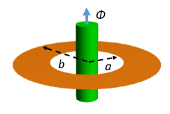
Figure 1: Two-dimensional ring threaded by a magnetic flux.

We assume that the field is confined in the spatial region bounded by two concentric circles having radii $a$ and $b$, $a<b$ (two-dimensional ring, see figure 1). On the edges of this region the field operator obeys the MIT bag boundary conditions

$$\left(1+in_{\mu}\gamma^{\mu}\right)\psi(x)=0,\;r=a,b.$$ (2.2)

with $n_{\mu}$ being the outward pointing unit vector normal to the boundaries. In the region $a\leqslant r\leqslant b$ one has $n_{\mu}=n_{u}\delta_{\mu}^{1}$ for the boundary at $r=u$ with

$$n_{a}=-1,\;n_{b}=1.$$ (2.3)

As a consequence of the boundary conditions (2.2), one gets $n_{\mu}\bar{\psi}\gamma^{\mu}\psi=0$ and the normal component of the fermionic current vanishes on the edges. Here and in what follows, $\bar{\psi}=\psi^{\dagger}\gamma^{0}$ is the Dirac adjoint and the dagger denotes Hermitian conjugation. This shows that the boundaries are impenetrable for the fermionic field. The boundary condition of the type (2.2) was used in the bag model of hadrons for the confinement of quarks [25]. The analog boundary condition in graphene physics is referred as the infinite mass boundary condition. It has been employed in (2+1)-dimensional Dirac theory for the breaking of time-reversal symmetry without magnetic fields [26]. Mainly motivated by the graphene physics, more general conditions for the Dirac equation, ensuring the absence of current normal to the boundary, have been discussed in [14, 27]. In (2+1)-dimensions, the most general energy-independent boundary condition contains four parameters.

For the further consideration we need to specify the representation for the Dirac matrices. In Cartesian coordinates, we take $\gamma^{(0)}=\sigma_{3}$, $\gamma^{(l)}=i\sigma_{l}$, $l=1,2$, where $\sigma_{1}$, $\sigma_{2}$, $\sigma_{3}$ are Pauli matrices. The Dirac matrices in cylindrical coordinates are obtained in the standard way by using the corresponding tetrad fields. They have the form $\gamma^{0}=\sigma_{3}$ and

$$\gamma^{l}=\frac{i^{2-l}}{r^{l-1}}\left(\begin{array}[]{cc}0&e^{-i\phi}\\ (-1)^{l-1}e^{i\phi}&0\end{array}\right),$$ (2.4)

for $l=1,2$. The corresponding spin connection vanishes, $\Gamma_{\mu}=0$. For the vector potential we will consider a configuration corresponding to the presence of a magnetic flux located in the region $r<a$. In the region under consideration, $a\leqslant r\leqslant b$, for the covariant components in the coordinates $(t,r,\phi)$ one has

$$A_{\mu}=(0,0,A_{2}).$$ (2.5)

Note that the physical azimuthal component for the vector potential is given by $A_{\phi}=-A_{2}/r$ and for the magnetic flux threading the ring we have $\Phi=-2\pi A_{2}$. Though the magnetic field strength for (2.5) vanishes, the magnetic flux enclosed by the ring gives rise to Aharonov-Bohm-like effects on physical observables, in particular for the VEVs. Note that the distribution of the magnetic flux in the region $r<a$ can be arbitrary. As the boundary $r=a$ is impenetrable for the fermionic field, the effect of the gauge field is purely topological and depends on the total flux alone. In this sense, the inner boundary can be viewed as a simplified model for a finite radius magnetic flux with the reflecting wall.

The zero-point fluctuations of the fermionic field $\psi(x)$ in the region $a\leqslant r\leqslant b$ are influenced by the magnetic flux threading the ring. As a consequence, the VEVs of physical quantities depend on the flux. This gives rise to a number of interesting physical phenomena, such as parity anomalies, formation of fermionic condensate and generation of quantum numbers. Here we are interested in the VEV of the fermionic current $j^{\mu}=\bar{\psi}\gamma^{\mu}\psi$. It appears as the source in the semiclassical Maxwell equations and, hence, it plays an important role in self-consistent dynamics involving the electromagnetic field. Let $S_{ik}^{(1)}(x,x^{\prime})=\langle 0|[\psi_{i}(x),\bar{\psi}_{k}(x^{\prime})]|0\rangle$ be the fermion two-point function, where $i$ and $k$ are spinor indices and $|0\rangle$ denotes the vacuum state. The VEV of the current density is expressed in terms of this function as

$$\langle j^{\mu}(x)\rangle\equiv\langle 0|j^{\mu}(x)|0\rangle=-\frac{e}{2}\mathrm{Tr}(\gamma^{\mu}S^{(1)}(x,x)),$$ (2.6)

with the trace over spinor indices understood. The expression in the right-hand side can be presented in the form of the sum over a complete set of positive- and negative-energy fermionic modes $\{\psi_{\sigma}^{(+)}(x),\psi_{\sigma}^{(-)}(x)\}$, specified by a set of quantum numbers $\sigma$. The mode functions $\psi_{\sigma}^{(\kappa)}(x)$, $\kappa=\pm$, obey the Dirac equation (2.1) and the boundary conditions (2.2). Expanding the field operator in terms of $\psi_{\sigma}^{(\kappa)}(x)$ and using the commutation relations for the annihilation and creation operators, for the VEV of the current density the following mode sum is obtained:

$$\langle j^{\mu}\rangle=-\frac{e}{2}\sum_{\sigma}\sum_{\kappa=-,+}\kappa\bar{\psi}_{\sigma}^{(\kappa)}(x)\gamma^{\mu}\psi_{\sigma}^{(\kappa)}(x).$$ (2.7)

Our prescription is to find the complete set of modes and to use this mode sum for the evaluation of the vacuum charge and current densities.

From the point of view of the renormalization of the VEVs, the important point here is that, owing to the flatness of the background spacetime and the zero field tensor for the external electromagnetic field in the region under consideration, for points outside the boundaries the structure of divergences is the same as for the (2+1)-dimensional boundary-free Minkowski spacetime in the absence of the magnetic flux. Consequently, the renormalization is reduced to the subtraction from the VEVs of the corresponding Minkowskian quantity. In problems of the quantum field theory with boundaries, one of the most efficient ways to extract from the VEVs the boundary-free part in a regularization independent way is based on the application of the Abel-Plana-type summation formulae to the corresponding mode sums (for the applications of the Abel-Plana formula and its generalizations in the theory of the Casimir effect see [15, 28]).

3 Fermionic modes

For the evaluation of the VEV in accordance with Eq. (2.7) we need to have the mode functions $\psi_{\sigma}^{(\pm)}(x)$ obeying the boundary conditions (2.2). Decomposing the spinor $\psi_{\sigma}^{(\kappa)}(x)$, $\kappa=\pm$, into upper and lower components, $\varphi_{+}$ and $\varphi_{-}$, respectively, from Eq. (2.1) we get the equations

$$\left(\partial_{0}\pm ism\right)\varphi_{\pm}\pm ie^{\mp i\phi}\left[\partial_{1}\mp i(\partial_{2}+i\alpha)/r\right]\varphi_{\mp}=0,$$ (3.1)

with the notation

$$\alpha=eA_{2}=-\Phi/\Phi_{0},$$ (3.2)

where $\Phi_{0}=2\pi/e$ is the elementary flux or the flux quantum. From Eq. (3.1) one finds the second-order differential equations for the separate components:

$$\left[\partial_{0}^{2}-\partial_{1}^{2}-\frac{1}{r}\partial_{1}-\frac{1}{r}(\partial_{2}+i\alpha)^{2}+m^{2}\right]\varphi_{\pm}=0.$$ (3.3)

Note that this equation is the same for both the components.

Let us present the solutions of these equations in the form

$$\varphi_{\pm}=\chi_{\pm}(r)e^{-\kappa iEt+i\left(j_{\pm}-1/2\right)\phi},$$ (3.4)

where $E>0$ and $j_{\pm}=\ldots,-3/2,-1/2,1/2,3/2,\ldots$. For the functions $\chi_{\pm}(r)$ we get the equations

$$\left(-\kappa E\pm sm\right)\chi_{\pm}e^{i\left(j_{\pm}\pm 1-j_{\mp}\right)\phi}\pm\left(\partial_{1}\pm\frac{j_{\pm}+\alpha-1/2}{r}\right)\chi_{\mp}=0.$$ (3.5)

and

$$\left[\partial_{1}^{2}+\frac{1}{r}\partial_{1}+\gamma^{2}-\frac{1}{r^{2}}\left(j_{\pm}+\alpha-1/2\right)^{2}\right]\chi_{\pm}(r)=0,$$ (3.6)

where $\gamma=\sqrt{E^{2}-m^{2}}$. From Eq. (3.5) it follows that $j_{-}=j_{+}+1$.

With this choice and denoting $j_{+}=j$, we take the solution for the function with the upper sign as

$$\chi_{+}(r)=Z_{\beta_{j}}(\gamma r)=c_{1}J_{\beta_{j}}(\gamma r)+c_{2}Y_{\beta_{j}}(\gamma r),$$ (3.7)

where $J_{\nu}(x)$ and $Y_{\nu}(x)$ are the Bessel and Neumann functions and

$$\beta_{j}=|j+\alpha|-\epsilon_{j}/2.$$ (3.8)

Here, $\epsilon_{j}=1$ for $j>-\alpha$, $\epsilon_{j}=-1$ for $j\leqslant-\alpha$. Note that $\epsilon_{j}\beta_{j}=j+\alpha-1/2$. By taking into account the recurrence relations for the cylinder functions, from Eq. (3.5) it follows that

$$\chi_{-}(r)=\frac{\epsilon_{j}\gamma}{\kappa E+sm}Z_{\beta_{j}+\epsilon_{j}}(\gamma r).$$ (3.9)

The ratio of the coefficients in the linear combination (3.7) is determined from the boundary condition (2.2) at $r=a$:

$$\frac{c_{2}}{c_{1}}=-\frac{J_{\beta_{j}}^{(a)}\left(\gamma a\right)}{Y_{\beta_{j}}^{(a)}\left(\gamma a\right)},$$ (3.10)

where and in what follows, for the Bessel and Neumann functions, we use the notation defined as

$$f_{\beta_{j}}^{(u)}\left(x\right) = xf_{\beta_{j}}^{\prime}\left(x\right)+[n_{u}(\kappa\sqrt{x^{2}+m_{u}^{2}}+sm_{u})-\epsilon_{j}\beta_{j}]f_{\beta_{j}}\left(x\right)$$ (3.11)

$$= n_{u}(\kappa\sqrt{x^{2}+m_{u}^{2}}+sm_{u})f_{\beta_{j}}\left(x\right)-\epsilon_{j}xf_{\beta_{j}+\epsilon_{j}}\left(x\right),$$

with $u=a,b$, $f=J,Y$, and $m_{u}=mu$. As a consequence, the mode functions are written in the form

$$\psi_{\sigma}^{(\kappa)}(x)=C_{\kappa}e^{-\kappa iEt+ij\phi}\left(\begin{array}[]{c}g_{\beta_{j},\beta_{j}}\left(\gamma a,\gamma r\right)e^{-i\phi/2}\\ \frac{\epsilon_{j}\gamma e^{i\phi/2}}{\kappa E+sm}g_{\beta_{j},\beta_{j}+\epsilon_{j}}\left(\gamma a,\gamma r\right)\end{array}\right),$$ (3.12)

where

$$g_{\beta_{j},\mu}(x,y)=Y_{\beta_{j}}^{(a)}\left(x\right)J_{\mu}\left(y\right)-J_{\beta_{j}}^{(a)}\left(x\right)Y_{\mu}\left(y\right).$$ (3.13)

We can check that the modes (3.12) are eigenfunctions of the total angular momentum operator $\hat{J}=-i(\partial_{2}+ieA)+\sigma_{3}/2$, for the eigenvalues $j+\alpha$:

$$\hat{J}\psi_{\sigma}^{(\kappa)}(x)=(j+\alpha)\psi_{\sigma}^{(\kappa)}(x).$$ (3.14)

Here, the part $\sigma_{3}/2$ corresponds to the pseudospin.

In a similar way, from the boundary condition (2.2) at $r=b$ we get $c_{2}/c_{1}=-J_{\beta_{j}}^{(b)}\left(\gamma b\right)/Y_{\beta_{j}}^{(b)}\left(\gamma b\right)$. Combining this with Eq. (3.10), one concludes that the eigenvalues for $\gamma$ in the region $a\leqslant r\leqslant b$ are the roots of the equation

$$C_{\beta_{j}}(\eta,\gamma a)\equiv J_{\beta_{j}}^{(a)}\left(\gamma a\right)Y_{\beta_{j}}^{(b)}\left(\gamma b\right)-J_{\beta_{j}}^{(b)}\left(\gamma b\right)Y_{\beta_{j}}^{(a)}\left(\gamma a\right)=0,$$ (3.15)

with $\eta=b/a$. The positive solutions of this equation with respect to $\gamma a$ will be denoted by $z_{l}$, $l=1,2,\ldots$, $z_{l}<z_{l+1}$. For the eigenvalues of $\gamma$ one has $\gamma=\gamma_{l}=z_{l}/a$. In this way, the mode functions are specified by the quantum numbers $\sigma=(l,j)$. Note that, the roots $z_{l}$ depend on the value of $j$ as well. In order to simplify the expressions below we do not write this dependence explicitly. For a given $j$, the equations (3.15) for the eigenvalues $\gamma_{l}$ of the positive- and negative-energy modes differ by the change of the energy sign, $E\rightarrow-E$ (through $\kappa$ in Eq. (3.11)). For the energy one has $E=\sqrt{\gamma_{l}^{2}+m^{2}}$. As we see, in the case of a massless field, the finite size effects induce a gap in the energy spectrum. The gap can be controlled by the geometrical characteristics of the model. Note that the gap generated by the finite size effects plays an important role in graphene made nanoribbons. In the problem at hand the size of the energy gap is determined by the minimal value of $\gamma_{l}$. For example, in the case $\alpha=1/3$, $j=1/2$ for the first root one has $z_{1}\approx 1.59$ for $b/a=2$ and $z_{1}\approx 0.81$ for $b/a=3$. The root increases with decreasing $b/a$ and with increasing $j$.

The function $C_{\beta_{j}}(\eta,x)$ in Eq. (3.15) can also be written in terms of the Hankel functions $H_{\beta_{j}}^{(1,2)}(x)$ as

$$C_{\nu}(\eta,x)=(i/2)\left[H_{\beta_{j}}^{(2a)}\left(x\right)H_{\beta_{j}}^{(1b)}\left(\eta x\right)-H_{\beta_{j}}^{(1a)}\left(x\right)H_{\beta_{j}}^{(2b)}\left(\eta x\right)\right],$$ (3.16)

with the notations defined as Eq. (3.11). With this representation, we can see that for a massless field the equation $C_{\beta_{j}}(\eta,\gamma a)=0$ is reduced to the one given in [29] for graphene rings described by the Dirac model with the infinite mass boundary condition on the edges. Note that to obtain an analytical approximation of the spectrum, in [29] the asymptotic form of the Hankel functions for large arguments was used. This approximation is valid for rings with the radius much larger than the width. As it will be shown below, the use of the generalized Abel-Plana formula allows us to obtain closed analytic expressions for the VEVs in the general case of geometrical characteristics of the ring.

For the complete specification of the mode functions (3.12) it remains to determine the coefficient $C_{\kappa}$. The latter is found from the orthonormalization condition

$$\int_{a}^{b}dr\int_{0}^{2\pi}d\phi\,r\psi_{\sigma}^{(\kappa)\dagger}(x)\psi_{\sigma^{\prime}}^{(\kappa)}(x)=\delta_{jj^{\prime}}\ \delta_{ll^{\prime}}.$$ (3.17)

Substituting the modes, using the result for the integral involving the square of cylinder functions (see [30]), after long but straightforward calculations one finds

$$\left|C_{\kappa}\right|^{2}=\frac{\pi z_{l}}{16a^{2}}\frac{E+\kappa sm}{E}T_{\beta_{j}}^{ab}(\eta,z_{l}).$$ (3.18)

Here, we have introduced the notation

$$T_{\beta_{j}}^{ab}(\eta,z)=z\left[D_{b}J_{\beta_{j}}^{(a)2}\left(z\right)/J_{\beta_{j}}^{(b)2}\left(\eta z\right)-D_{a}\right]^{-1},$$ (3.19)

with

$$D_{u}=u^{2}\frac{E+\kappa sm}{E}\left[E\left(E+\kappa n_{u}\frac{\epsilon_{j}\beta_{j}}{u}\right)+\kappa n_{u}\frac{E-\kappa sm}{2u}\right].$$ (3.20)

As it has been already mentioned, the eigenvalue equations (3.15) for the positive- and negative-energy modes are obtained from each other by the change of the energy sign. Redefining the azimuthal quantum number in accordance with $j\rightarrow-j$, the negative-energy modes can also be written in the form

$$\psi_{\sigma}^{(-)}=C_{-}^{\prime}e^{iEt-ij\phi}\left(\begin{array}[]{c}\frac{\epsilon_{j}^{-}\gamma e^{-i\phi/2}}{E+sm}g_{\beta_{j}^{-},\beta_{j}^{-}+\epsilon_{\lambda_{n}^{-}}}(\gamma a,\gamma r)\\ g_{\beta_{j}^{-},\beta_{j}^{-}}(\gamma a,\gamma r)e^{i\phi/2}\end{array}\right),$$ (3.21)

where $\beta_{j}^{-}=|j-\alpha|-\epsilon_{j}^{-}/2$, $\epsilon_{j}^{-}=1$ for $j>\alpha$ and $\epsilon_{j}^{-}=-1$ for $j\leqslant\alpha$. In the definition (3.13) of the function $g_{\beta_{j}^{-},\mu}(x,y)$ the notations $f_{\beta_{j}^{-}}^{(u)}\left(x\right)$ are defined as Eq. (3.11) with $\kappa=1$ (as in the case of the positive-frequency functions). With the modes (3.21), the eigenvalues for $\gamma$ are solutions of the equation

$$J_{\beta_{j}^{-}}^{(a)}\left(\gamma a\right)Y_{\beta_{j}^{-}}^{(b)}\left(\gamma b\right)-Y_{\beta_{j}^{-}}^{(a)}\left(\gamma a\right)J_{\beta_{j}^{-}}^{(b)}\left(\gamma b\right)=0.$$ (3.22)

Because now the functions $f_{\nu}^{(u)}\left(x\right)$ are the same for the positive- and negative-energy modes, Eq. (3.22) differs from the corresponding equation (3.15) for the positive-energy modes just by the sign of $\alpha$, $\alpha\rightarrow-\alpha$. It can be seen that the normalization constant $C_{-}^{\prime}$ is given by the expression in the right-hand side of Eq. (3.18) with $\kappa=1$ and with $z_{l}=\gamma a$ being the roots of Eq. (3.22). Of course, in the evaluation of the VEVs we can use both types of the modes.

4 Charge density

We start our consideration of the VEVs with the charge density. Substituting the mode functions (3.12) into the mode-sum formula (2.7) we get

$$\langle j^{0}\rangle=-\frac{\pi e}{32a^{2}}\sum_{j}\sum_{l=1}^{\infty}\sum_{\kappa=\pm}\,\kappa T_{\beta_{j}}^{ab}(\eta,z_{l})h_{0}(z_{l}),$$ (4.1)

where $\sum_{j}$ stands for the summation over $j=\pm 1/2,\pm 3/2,\ldots$, and

$$h_{0}(z)=\frac{z}{E}\left[\left(E+\kappa sm\right)g_{\beta_{j},\beta_{j}}^{2}(z,zr/a)+\left(E-\kappa sm\right)g_{\beta_{j},\beta_{j}+\epsilon_{j}}^{2}(z,zr/a)\right],$$ (4.2)

with $E=\sqrt{z^{2}/a^{2}+m^{2}}$. In Eq. (4.1), the eigenvalues $z_{l}$ are given implicitly, as roots of Eq. (3.15), and this representation is not convenient for the further evaluation of the VEV. Another disadvantage of the representation (4.1) is that the separate terms in the series are highly oscillating for large values of the quantum numbers.

These difficulties are overcome by using for the summation over $l$ the Abel-Plana-type formula

$$\sum_{l=1}^{\infty}h(z_{l})T_{\beta_{j}}^{ab}(\eta,z_{l})=\frac{4}{\pi^{2}}\int_{0}^{\infty}{dz\,}\frac{h(z)}{J_{\beta_{j}}^{(a)2}\left(z\right)+Y_{\beta_{j}}^{(a)2}\left(z\right)}$$

$$\qquad-\frac{2}{\pi}\underset{z=0}{\mathrm{Res}}\left[\frac{h(z)H_{\beta_{j}}^{(1b)}\left(\eta z\right)}{C_{\beta_{j}}(\eta,z)H_{\beta_{j}}^{(1a)}\left(z\right)}\right]-\frac{1}{\pi}\int_{0}^{\infty}dz\,\sum_{p=+,-}\Omega_{a\beta_{j}}^{(p)}(z,\eta z)h(ze^{pi\frac{\pi}{2}}),$$ (4.3)

where

$$\Omega_{a\beta_{j}}^{(p)}(z,\eta z)=\frac{K_{\beta_{j}}^{(bp)}(\eta z)/K_{\beta_{j}}^{(ap)}(z)}{K_{\beta_{j}}^{(ap)}\left(z\right)I_{\beta_{j}}^{(bp)}\left(\eta z\right)-I_{\beta_{j}}^{(ap)}(z)K_{\beta_{j}}^{(bp)}(\eta z)}.$$ (4.4)

Here we have introduced the notation

$$f_{\beta_{j}}^{(up)}(x)=xf_{\beta_{j}}^{\prime}\left(x\right)+\left\{n_{u}\left[\kappa\sqrt{\left(xe^{p\pi i/2}\right)^{2}+m_{u}^{2}}+sm_{u}\right]-\epsilon_{j}\beta_{j}\right\}f_{\beta_{j}}\left(x\right),$$ (4.5)

with $f=I,K$ for the modified Bessel functions $I_{\beta_{j}}\left(x\right)$ and $K_{\beta_{j}}\left(x\right)$. The formula (4.3) is valid for a function $h(z)$ analytic in the complex half-plane Re$\,z>0$, $z=x+iy$, and obeying the condition $|h(z)|<\varepsilon(x)e^{c|y|}$, where $c<2(\eta-1)$ and $\varepsilon(x)/x\rightarrow 0$ for $x\rightarrow+\infty$. On the imaginary axis the function $h(z)$ may have branch points. The summation formula (4.3) is obtained from the generalized Abel-Plana formula [28] (see also [31]). Note that for the square root in Eq. (4.5) one has

$$\sqrt{\left(ze^{p\pi i/2}\right)^{2}+m_{u}^{2}}=\left\{\begin{array}[]{cc}\sqrt{m_{u}^{2}-z^{2}},&z<m_{u}\\ pi\sqrt{z^{2}-m_{u}^{2}},&z>m_{u}\end{array}\right..$$ (4.6)

In particular, we see that $f_{\beta_{j}}^{(u+)}(z)=f_{\beta_{j}}^{(u-)}(z)$ for $z<m_{u}$. From here it follows that $\Omega_{a\beta_{j}}^{(-)}(z,\eta z)=\Omega_{a\beta_{j}}^{(+)}(z,\eta z)$ for $z<ma$.

For the charge density the function $h(z)$ in the summation formula (4.3) is specified by Eq. (4.2). This function has branch points $z=\pm ima$ on the imaginary axis. For $z<ma$ one has the relation $h_{0}(ze^{-\pi i/2})=-h_{0}(ze^{\pi i/2})$ and, hence, in the last integral of Eq. (4.3) the part over the region $[0,ma]$ becomes zero. For $z>ma$ we find

$$h_{0}(ze^{pi\frac{\pi}{2}})=\frac{4z}{\pi^{2}}\left[\left(\frac{\kappa sm}{\sqrt{z^{2}/a^{2}-m^{2}}}+pi\right)G_{\beta_{j},\beta_{j}}^{(ap)2}(z,zr/a)+\left(\frac{\kappa sm}{\sqrt{z^{2}/a^{2}-m^{2}}}-pi\right)G_{\beta_{j},\beta_{j}+\epsilon_{j}}^{(ap)2}(z,zr/a)\right],$$ (4.7)

with the function

$$G_{\beta_{j},\mu}^{(ap)}(x,y)=K_{\beta_{j}}^{(ap)}\left(x\right)I_{\mu}\left(y\right)-(-1)^{\mu-\beta_{j}}I_{\beta_{j}}^{(ap)}\left(x\right)K_{\mu}\left(y\right).$$ (4.8)

Substituting Eq. (4.7) into Eq. (4.3) and then into Eq. (4.1), we can see that $\kappa$ and $p$ enter into the expression of the part corresponding to the last term in the right-hand side of Eq. (4.3) in the form of the product $\kappa p$. From here it follows that the positive- and negative-energy modes give the same contributions to this part of the charge density.

After all these transformations, the VEV of the charge density is presented in the form

$$\langle j^{0}\rangle = \langle j^{0}\rangle_{a}+\frac{e}{2\pi^{2}}\sum_{j}\,\int_{m}^{\infty}dx\,x\left\{\frac{sm}{\sqrt{x^{2}-m^{2}}}\right.$$ (4.9)

$$\times\mathrm{Re}\left[\Omega_{a\beta_{j}}(ax,bx)\left(G_{\beta_{j},\beta_{j}}^{(a)2}(ax,rx)+G_{\beta_{j},\beta_{j}+\epsilon_{j}}^{(a)2}(ax,rx)\right)\right]$$

$$\left.-\mathrm{Im}\left[\Omega_{a\beta_{j}}(ax,bx)\left(G_{\beta_{j},\beta_{j}}^{(a)2}(ax,rx)-G_{\beta_{j},\beta_{j}+\epsilon_{j}}^{(a)2}(ax,rx)\right)\right]\right\},$$

where

$$\langle j^{0}\rangle_{a}=-\frac{e}{8\pi a^{2}}\sum_{j}\sum_{\kappa=\pm 1}\,\int_{0}^{\infty}{dz\,}\frac{\kappa h_{0}(z)}{J_{\beta_{j}}^{(a)2}\left(z\right)+Y_{\beta_{j}}^{(a)2}\left(z\right)}.$$ (4.10)

The new notations are defined as

$$\Omega_{a\beta_{j}}(ax,bx)=\frac{K_{\beta_{j}}^{(b)}(bx)/K_{\beta_{j}}^{(a)}(ax)}{K_{\beta_{j}}^{(a)}\left(ax\right)I_{\beta_{j}}^{(b)}\left(bx\right)-I_{\beta_{j}}^{(a)}(ax)K_{\beta_{j}}^{(b)}(bx)},$$ (4.11)

and

$$G_{\beta_{j},\mu}^{(u)}(x,y)=K_{\beta_{j}}^{(u)}\left(x\right)I_{\mu}\left(y\right)-(-1)^{\mu-\beta_{j}}I_{\beta_{j}}^{(u)}\left(x\right)K_{\mu}\left(y\right),$$ (4.12)

with $u=a,b$ (the function $G_{\beta_{j},\mu}^{(b)}(x,y)$ is used below). For the modified Bessel functions now we use the notations

$$f_{\beta_{j}}^{(u)}(z) = zf_{\beta_{j}}^{\prime}\left(z\right)+\left[n_{u}\left(i\sqrt{z^{2}-m_{u}^{2}}+sm_{u}\right)-\epsilon_{j}\beta_{j}\right]f_{\beta_{j}}\left(z\right)$$ (4.13)

$$= \delta_{f}zf_{\beta_{j}+\epsilon_{j}}\left(z\right)+n_{u}(i\sqrt{z^{2}-m_{u}^{2}}+sm_{u})f_{\beta_{j}}\left(z\right),$$

where $f=I,K$, $\delta_{I}=1$ and $\delta_{K}=-1$.

Let us present the parameter $\alpha$ from Eq. (3.2), related to the magnetic flux threading the ring, in the form

$$\alpha=N+\alpha_{0},\;|\alpha_{0}|\leqslant 1/2,$$ (4.14)

where $N$ is an integer. Redefining the summation variable $j$ in accordance with $j+N\rightarrow j$ we see that the charge density does not depend on the integer part $N$. Then, separating the summations over negative and positive values of $j$, making the replacement $j\rightarrow-j$ in the part with negative $j$ and introducing a new summation variable $n=j-1/2$, the charge density is presented as

$$\langle j^{0}\rangle = \langle j^{0}\rangle_{a}+\frac{e}{2\pi^{2}}\sum_{n=0}^{\infty}\,\sum_{p=\pm}p\int_{m}^{\infty}dx\,x\left\{\frac{sm}{\sqrt{x^{2}-m^{2}}}\right.$$ (4.15)

$$\times\mathrm{Re}\left[\Omega_{an_{p}}(ax,bx)\left(G_{n_{p},n_{p}}^{(a)2}(ax,rx)+G_{n_{p},n_{p}+1}^{(a)2}(ax,rx)\right)\right]$$

$$\left.+\mathrm{Im}\left[\Omega_{an_{p}}(ax,bx)\left(G_{n_{p},n_{p}+1}^{(a)2}(ax,rx)-G_{n_{p},n_{p}}^{(a)2}(ax,rx)\right)\right]\right\},$$

with

$$n_{p}=n+p\alpha_{0},$$ (4.16)

and now the notation (4.13) in the definitions (4.11) and (4.12) for $\Omega_{an_{p}}(ax,bx)$ and $G_{n_{p},\mu}^{(a)}(ax,rx)$ is specified to

$$f_{n_{p}}^{(u)}(z)=\delta_{f}zf_{n_{p}+1}\left(z\right)+n_{u}(sm_{u}+i\sqrt{z^{2}-m_{u}^{2}})f_{n_{p}}\left(z\right),$$ (4.17)

for $f=I,K$. The representation (4.15) explicitly shows that the last term is an odd function of the fractional part $\alpha_{0}$. The property that the VEVs do not depend on the integer part of the flux, in units of the flux quantum, is a general feature in the Aharonov-Bohm effect and is a consequence of that the flux enters through the phase of the wavefunction.

The last term in Eq. (4.15) vanishes in the limit $b\rightarrow\infty$ (for large values $b$ the function $\Omega_{an_{p}}(ax,bx)$ falls off as $e^{-2bx}$). From here it follows that the part (4.10) is the charge density in the region $r\geqslant a$ for the geometry of a single boundary at $r=a$. In order to extract from that part the boundary-induced effects we further transform the expression (4.10), with $h_{0}(z)$ form (4.2), by using the relation

$$\frac{g_{\beta_{j},\lambda}^{2}(z,y)}{J_{\beta_{j}}^{(a)2}(z)+Y_{\beta_{j}}^{(a)2}(z)}=J_{\lambda}^{2}(y)-\frac{1}{2}\sum_{l=1,2}\frac{J_{\beta_{j}}^{(a)}(z)}{H_{\beta_{j}}^{(la)}(z)}H_{\lambda}^{(l)2}(y),$$ (4.18)

with $\lambda=\beta_{j},\beta_{j}+\epsilon_{j}$. Substituting into Eq. (4.10), in the part with the Hankel functions, we rotate the contour of the integration over $z$ by the angles $\pi/2$ and $-\pi/2$ for the terms with $l=1$ and $l=2$, respectively. The integrals over the segments $[0,im_{a}]$ and $[0,-im_{a}]$ cancel each other and, introducing the modified Bessel functions, again, we can see that the contributions coming from the positive- and negative-energy modes coincide. As a result, for the contribution (4.10), we come to the decomposition

$$\langle j^{0}\rangle_{a}=\langle j^{0}\rangle_{0}+\langle j^{0}\rangle_{a}^{\mathrm{(b)}},$$ (4.19)

where

$$\langle j^{0}\rangle_{0}=-\frac{e}{8\pi}\sum_{j}\sum_{\kappa=\pm}\,\kappa\int_{0}^{\infty}dx\,x\left[\left(1+\frac{s\kappa m}{\sqrt{x^{2}+m^{2}}}\right)J_{\beta_{j}}^{2}(xr)+\left(1-\frac{s\kappa m}{\sqrt{x^{2}+m^{2}}}\right)J_{\beta_{j}+\epsilon_{j}}^{2}(xr)\right],$$ (4.20)

and

$$\langle j^{0}\rangle_{a}^{\mathrm{(b)}} = \frac{e}{2\pi^{2}}\sum_{j}\,\int_{m}^{\infty}dx\,x\left\{sm\frac{K_{\beta_{j}}^{2}(rx)+K_{\beta_{j}+\epsilon_{j}}^{2}(rx)}{\sqrt{x^{2}-m^{2}}}\mathrm{Re}\left[\frac{I_{\beta_{j}}^{(a)}(ax)}{K_{\beta_{j}}^{(a)}(ax)}\right]\right.$$ (4.21)

$$\left.+\left[K_{\beta_{j}+\epsilon_{j}}^{2}(rx)-K_{\beta_{j}}^{2}(rx)\right]\mathrm{Im}\left[\frac{I_{\beta_{j}}^{(a)}(ax)}{K_{\beta_{j}}^{(a)}(ax)}\right]\right\},$$

with the notations (4.13). For the representation $s=1$, this expression for a single boundary-induced part coincides with the one given in Ref. [22] (the sign difference is related to that in [22], for the evaluation of the VEVs, the analog of the negative-energy mode functions (3.21) for the geometry with a single boundary was used with $\alpha$ replaced by $-\alpha$; hence, in comparing the formulas here with the results of [22], the replacements $\alpha\rightarrow-\alpha$ and $\alpha_{0}\rightarrow-\alpha_{0}$ should be made).

In order to give a physical interpretation of the separate terms in Eq. (4.19) let us consider the limit $a\rightarrow 0$. Note that the radius of the magnetic flux should also be taken to zero. For $j+\alpha\neq 0$ one has

$$\frac{I_{\beta_{j}}^{(a)}(ax)}{K_{\beta_{j}}^{(a)}(ax)}\approx\frac{i\sqrt{x^{2}-m^{2}}+\epsilon_{j}sm}{x}\frac{2\left(ax/2\right)^{2|j+\alpha|}}{\Gamma^{2}(|j+\alpha|+1/2)},$$ (4.22)

and, hence, the part (4.21) vanishes as $a^{2|j+\alpha|}$. For half-odd integer values of $\alpha$, the exceptional case corresponds to the mode with $j=-\alpha$. For this mode $\beta_{j}=1/2$, $\epsilon_{j}=-1$, and we get

$$\frac{I_{\beta_{j}}^{(a)}(ax)}{K_{\beta_{j}}^{(a)}(ax)}\approx\frac{2}{\pi}\frac{i\sqrt{x^{2}-m^{2}}-sm}{x}.$$ (4.23)

Note that for this special value of $\beta_{j}$, in Eq. (4.21) the coefficient of the term with the imaginary part of Eq. (4.23) vanishes.

Hence, if $\alpha$ is not a half-odd integer one has

$$\lim_{a\rightarrow 0}\langle j^{0}\rangle_{a}=\langle j^{0}\rangle_{0}.$$ (4.24)

In this case, the part (4.21) in the VEV of the charge density is induced by the presence of the boundary at $r=a$, whereas $\langle j^{0}\rangle_{0}$ gives the charge density in the boundary-free geometry with a point like magnetic flux at $r=0$. For $\alpha$ being a half-odd integer, by using (4.23), from Eq. (4.21) one gets

$$\lim_{a\rightarrow 0}\langle j^{0}\rangle_{a}=\langle j^{0}\rangle_{0}+\frac{em}{\pi^{2}r}\,\int_{0}^{\infty}dy\,\frac{e^{-2mr\sqrt{y^{2}+1}}}{y^{2}+1}.$$ (4.25)

For a massless field the last term in this expression vanishes and we come to the same interpretation of the separate terms in Eq. (4.19).

The boundary-induced contribution (4.21) does not depend on the integer part $N$ in Eq. (4.14). Redefining the summation variable in Eq. (4.21), this contribution is rewritten in the form

$$\langle j^{0}\rangle_{a}^{\mathrm{(b)}} = \frac{e}{2\pi^{2}}\sum_{n=0}^{\infty}\,\sum_{p=-,+}p\int_{m}^{\infty}dx\,x$$ (4.26)

$$\times\left\{sm\frac{K_{n_{p}}^{2}(rx)+K_{n_{p}+1}^{2}(rx)}{\sqrt{x^{2}-m^{2}}}\mathrm{Re}\left[\frac{I_{n_{p}}^{(a)}(ax)}{K_{n_{p}}^{(a)}(ax)}\right]\right.$$

$$\left.+\left[K_{n_{p}+1}^{2}(rx)-K_{n_{p}}^{2}(rx)\right]\mathrm{Im}\left[\frac{I_{n_{p}}^{(a)}(ax)}{K_{n_{p}}^{(a)}(ax)}\right]\right\},$$

with $n_{p}$ given by Eq. (4.16). This explicitly shows that the single boundary-induced charge density is an odd function of $\alpha_{0}$. The real and imaginary parts in Eq. (4.26) are explicitly given by the relation

$$\frac{I_{n_{p}}^{(u)}(z)}{K_{n_{p}}^{(u)}(z)}=\frac{W_{n_{p}}^{(u)}(z)-in_{u}\sqrt{1-m_{u}^{2}/z^{2}}}{z[K_{n_{p}+1}^{2}\left(z\right)+K_{n_{p}}^{2}\left(z\right)]-2sn_{u}m_{u}K_{n_{p}}\left(z\right)K_{n_{p}+1}\left(z\right)},$$ (4.27)

with $u=a,b$ and with the function

$$W_{\nu}^{(u)}(z) = z\left[I_{\nu}\left(z\right)K_{\nu}\left(z\right)-I_{\nu+1}\left(z\right)K_{\nu+1}\left(z\right)\right]$$ (4.28)

$$+n_{u}sm_{u}\left[I_{\nu+1}\left(z\right)K_{\nu}\left(z\right)-I_{\nu}\left(z\right)K_{\nu+1}\left(z\right)\right].$$

Note that for $z\geqslant m_{u}$ the denominator in Eq. (4.27) is positive. For a massless field and at large distances from the boundary, $r\gg a$, the dominant contribution to the boundary-induced part (4.26) comes from the term $n=0$ and this part decays as $(a/r)^{3-2|\alpha_{0}|}$ with the sign $\mathrm{sgn}(\alpha_{0})\langle j^{0}\rangle_{a}^{\mathrm{(b)}}/e<0$. For a massive field and for $r\gg a,m^{-1}$, the dominant contribution in Eq. (4.26) comes from the region near the lower limit of the integration and the boundary-induced charge density is suppressed by the factor $e^{-2mr}/r^{3/2}$.

From the consideration above it follows that, if $|\alpha_{0}|\neq 1/2$, the part $\langle j^{0}\rangle_{0}$ can be interpreted as the charge density in boundary-free two-dimensional space with a special type of boundary condition on the magnetic flux line at $r=0$. Namely, we impose the bag boundary condition at finite radius which is then taken to zero. Consequently, the part (4.26) is interpreted as the contribution induced in the region $a\leqslant r<\infty$ by the boundary $r=a$. The last term in Eq. (4.15) is the contribution in the charge density induced when we add the boundary at $r=b$ to the geometry with a single boundary at $r=a$. In this sense, this part can be termed as the second boundary-induced contribution.

The expression (4.20) for the boundary-free part can be further simplified. The first terms in the brackets of the coefficients of the functions $J_{\beta_{j}}^{2}(xr)$ and $J_{\beta_{j}+\epsilon_{j}}^{2}(xr)$ are canceled for the contributions coming from the positive- and negative-energy modes. For the remaining part we get

$$\langle j^{0}\rangle_{0}=\frac{esm}{4\pi}\sum_{j}\,\int_{0}^{\infty}dx\,x\frac{J_{\beta_{j}+\epsilon_{j}}^{2}(xr)-J_{\beta_{j}}^{2}(xr)}{\sqrt{x^{2}+m^{2}}},$$ (4.29)

that is further simplified to

$$\langle j^{0}\rangle_{0}=\frac{esm}{4\pi}\,\int_{0}^{\infty}dx\,x\frac{J_{-\alpha_{0}}^{2}(xr)-J_{\alpha_{0}}^{2}(xr)}{\sqrt{x^{2}+m^{2}}}.$$ (4.30)

This expression with $s=1$ was obtained in [10, 12]. After the rotation of the integration contour, it can also be presented in the form [10, 12]

$$\langle j^{0}\rangle_{0}=\frac{esm^{2}}{\pi^{3}}\sin\left(\pi\alpha_{0}\right)\int_{1}^{\infty}dx\frac{xK_{\alpha_{0}}^{2}(mrx)}{\sqrt{x^{2}-1}}.$$ (4.31)

An equivalent expression for the boundary-free part is provided in Ref. [22]:

$$\langle j^{0}\rangle_{0}=\frac{esm}{2\pi^{2}r}\sin\left(\pi\alpha_{0}\right)\int_{0}^{\infty}dx\,\frac{\cosh(2\alpha_{0}x)}{\cosh x}e^{-2mr\cosh x}.$$ (4.32)

Similarly to the boundary-induced contributions, this part is an odd function of the parameter $\alpha_{0}$. For a massless field the boundary-free contribution in the charge density vanishes for $r\neq 0$. In the case of a massive field, at large distances, the charge density $\langle j^{0}\rangle_{0}$ falls off as $e^{-2mr}/r^{3/2}$, whereas at the origin it diverges as $1/r$. At large distances, the decaying factor for a massive field is the same as that for the boundary-induced contribution (4.26).

The charge density (4.31) for the boundary-free geometry with a point like magnetic flux corresponds to a special boundary condition on the fermion field at the location of the flux. In general, the self-adjoint extension procedure for the Dirac Hamiltonian leads to a one-parameter family of boundary conditions [32]. The value of the parameter in the boundary condition is determined by the physical details of the magnetic field distribution inside a more realistic finite radius flux tube (see, e.g., [33] for models with finite radius magnetic flux).

Combining all the results given above, we conclude that the total charge density $\langle j^{0}\rangle$ in the region $a\leqslant r\leqslant b$ is a periodic odd function of the magnetic flux threading the ring, with the period equal to the flux quantum. As a function of the parameter $\alpha$ (magnetic flux in units of the flux quantum), the charge density (4.32) in the boundary-free geometry is discontinuous at the half-odd integer values $\alpha=N+1/2$:

$$\lim_{\alpha_{0}\rightarrow\pm 1/2}\langle j^{0}\rangle_{0}=\pm\frac{esm}{2\pi^{2}r}K_{0}(2mr).$$ (4.33)

In the geometry with a single boundary at $r=a$, it can be seen that for the boundary-induced contribution in the region $r\geqslant a$ one has $\lim_{\alpha_{0}\rightarrow\pm 1/2}\langle j^{0}\rangle_{a}^{\mathrm{(b)}}=-\lim_{\alpha_{0}\rightarrow\pm 1/2}\langle j^{0}\rangle_{0}$. This means that, in this geometry, the total charge density vanishes for $\alpha=N+1/2$, $\lim_{\alpha_{0}\rightarrow\pm 1/2}\langle j^{0}\rangle_{a}=0$, and it is a continuous function of the magnetic flux everywhere. It can be checked that, in the expression (4.15) for the total charge in the ring geometry the last term vanishes in the limits $\alpha_{0}\rightarrow\pm 1/2$ (the real and imaginary parts in Eq. (4.15) vanish separately) and, hence, similarly to the single boundary part, the total charge density $\langle j^{0}\rangle$ is a continuous function at the half-odd integer values of $\alpha$.

Having discussed general features of the charge density, for the further clarification of the dependence on the parameters of the model, let us consider numerical examples. In the left panel of figure 2, for the geometry of two boundaries at $r=a,b$, we have plotted the charge density as a function of the radial coordinate for a massless fermionic field and for $\alpha_{0}=1/4$. The numbers near the curves are the values of the ratio $b/a$. The dashed curve presents the charge density in the geometry of a single boundary at $r=a$, namely, the quantity $10^{3}a^{2}\langle j^{0}\rangle_{a}^{\mathrm{(b)}}/e$. In the right panel of figure 2, by the full curves, the charge density is plotted as a function of $\alpha_{0}$ for fixed values $ma=0.1$, $b/a=8$, $r/a=2$. The numbers near the curves are the values of the parameter $s$. The dashed curve is the corresponding charge density for a massless field with the same values of the other parameters. As is seen from the left panel, the charge density is peaked around the inner edge of the ring. The ratio $\langle j^{0}\rangle/e$ is negative near the inner edge and positive near the outer edge. In the geometry of a single boundary at $r=a$ this ratio is negative for $\alpha_{0}>0$. We have already mentioned that the charge density vanishes for $|\alpha_{0}|=1/2$, a feature seen from figure 2.

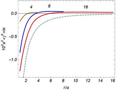
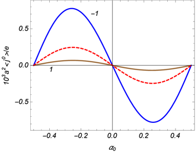
Figure 2: Charge density in the ring as a function of the radial coordinate for a massless field (left panel) and as a function of the parameter $\alpha_{0}$ (right panel). The left panel is plotted for the magnetic flux parameter $\alpha_{0}=1/4$ and the numbers near the curves are the values of $b/a$. The dashed curve in that panel corresponds to the charge density outside a single boundary at $r=a$. The full curves in the right panel are plotted for $ma=0.1$, $b/a=8$, $r/a=2$ and the numbers near the curves are the values of $s$. The dashed curve in the right panel corresponds to a massless field.

In figure 3 the charge density is displayed versus the ratio $b/a$ for fixed values $\alpha_{0}=1/4$, $r/a=1.5$. The numbers near the curves are the values of the parameter $ma$. The dashed lines correspond to the current density outside a single boundary of radius $a$. For the left and right panels $s=1$ and $s=-1$, respectively. Note that the scaling factors for these panels are different. The charge density for the representation $s=-1$ is essentially larger. The general feature seen from figure 3 is that the presence of the outer edge leads to the decrease of the absolute value of the charge density. For large values of $b/a$, the approach of the charge density in the ring geometry to the corresponding quantity in the geometry with a single edge is quicker with increasing mass.

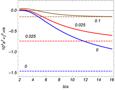
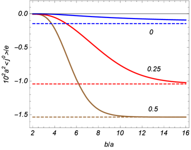
Figure 3: The dependence of the charge density on the ratio $b/a$ for irreducible representations $s=1$ (left panel) and $s=-1$ (right panel). The graphs are plotted for $\alpha_{0}=1/4$, $r/a=1.5$ and the numbers near the curves are the values for $ma$. The horizontal dashed curves correspond to the charge density in the geometry of a single boundary at $r=a$.

From figures 2 and 3 we see that the behavior of the charge density when the parameter $ma$ increases from $ma=0$ is essentially different for the representations $s=1$ and $s=-1$. With the initial increase of $ma$, the modulus of the charge density decreases for the former case and increases for the latter one. Of course, we expect that for $ma\gg 1$ the charge density will be suppressed for both the cases. This is seen from figure 4. It presents the dependence of the charge density on the mass of the field for irreducible representations $s=1$ (left panel) and $s=-1$ (right panel). The graphs are plotted for $\alpha_{0}=1/4$, $b/a=8$, $r/a=2$. The dashed curves correspond to the charge density in the geometry of a single boundary at $r=a$. The dotted line in the right panel is the charge density for $s=-1$ in the boundary-free problem. The corresponding charge density for $s=1$ differs by the sign. The suppression of the VEV with increasing $ma$ is stronger in the case $s=1$.

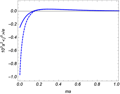
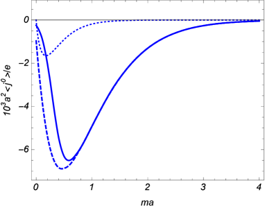
Figure 4: Charge density as a function of the field mass (in units of $1/a$) for fields with $s=1$ (left panel) and $s=-1$ (right panel). For the values of the parameters we have taken $\alpha_{0}=1/4$, $b/a=8$, $r/a=2$. The dashed curves present the charge density outside a single boundary at $r=a$. The dotted line corresponds to the charge density in the boundary-free geometry.

The representation (4.15) for the charge density in the ring is not symmetric with respect to the inner and outer edges. An alternative representation, with the extracted outer boundary part is obtained from Eq. (4.9) by making use of the relation

$$\frac{I_{n_{p}}^{(a)}(ax)}{K_{n_{p}}^{(a)}(ax)}K_{\mu}^{2}(rx)=\frac{K_{n_{p}}^{(b)}(bx)}{I_{n_{p}}^{(b)}(bx)}I_{\mu}^{2}(rx)+\sum_{u=a,b}n_{u}\Omega_{un_{p}}(ax,bx)G_{n_{p},\mu}^{(u)2}(ux,rx),$$ (4.34)

with the notation

$$\Omega_{bn_{p}}(ax,bx)=\frac{I_{n_{p}}^{(a)}(ax)/I_{n_{p}}^{(b)}(bx)}{K_{n_{p}}^{(a)}\left(ax\right)I_{n_{p}}^{(b)}\left(bx\right)-I_{n_{p}}^{(a)}(ax)K_{n_{p}}^{(b)}(bx)}.$$ (4.35)

The expression for the charge density takes the form

$$\langle j^{0}\rangle = \langle j^{0}\rangle_{b}+\frac{e}{2\pi^{2}}\sum_{n=0}^{\infty}\sum_{p=\pm}p\,\int_{m}^{\infty}dx\,x\left\{\frac{sm}{\sqrt{x^{2}-m^{2}}}\right.$$ (4.36)

$$\times\mathrm{Re}\left[\Omega_{bn_{p}}(ax,bx)\left(G_{n_{p},n_{p}}^{(b)2}(bx,rx)+G_{n_{p},n_{p}+1}^{(b)2}(bx,rx)\right)\right]$$

$$\left.+\mathrm{Im}\left[\Omega_{bn_{p}}(ax,bx)\left(G_{n_{p},n_{p}+1}^{(b)2}(bx,rx)-G_{n_{p},n_{p}}^{(b)2}(bx,rx)\right)\right]\right\}.$$

Here, the first term in the right-hand side is decomposed as

$$\langle j^{0}\rangle_{b}=\langle j^{0}\rangle_{0}+\langle j^{0}\rangle_{b}^{\mathrm{(b)}},$$ (4.37)

with

$$\langle j^{0}\rangle_{b}^{\mathrm{(b)}} = \frac{e}{2\pi^{2}}\sum_{n=0}^{\infty}\sum_{p=\pm}p\,\,\int_{m}^{\infty}dx\,x\left\{sm\frac{I_{n_{p}}^{2}(rx)+I_{n_{p}+1}^{2}(rx)}{\sqrt{x^{2}-m^{2}}}\mathrm{Re}\left[\frac{K_{n_{p}}^{(b)}(bx)}{I_{n_{p}}^{(b)}(bx)}\right]\right.$$ (4.38)

$$\left.+\left[I_{n_{p}+1}^{2}(rx)-I_{n_{p}}^{2}(rx)\right]\mathrm{Im}\left[\frac{K_{n_{p}}^{(b)}(bx)}{I_{n_{p}}^{(b)}(bx)}\right]\right\},$$

and with the notations defined in accordance with Eq. (4.17). For the ratio under the signs of the real and imaginary parts in Eq. (4.38) we have the following explicit expression

$$\frac{K_{n_{p}}^{(u)}(z)}{I_{n_{p}}^{(u)}(z)}=\frac{W_{n_{p}}^{(u)}(z)+in_{u}\sqrt{1-m_{u}^{2}/z^{2}}}{z[I_{n_{p}+1}^{2}\left(z\right)+I_{n_{p}}^{2}\left(z\right)]+2n_{u}sm_{u}I_{n_{p}}\left(z\right)I_{n_{p}+1}\left(z\right)}.$$ (4.39)

The denominator in this expression is positive for $z\geqslant m_{u}$. Relatively simple expressions for single boundary parts (4.26) and (4.38) are obtained for a massless field.

If $|\alpha_{0}|\neq 1/2$, in the limit $a\rightarrow 0$ one has

$$\Omega_{bn_{p}}(az,bz)\approx\frac{I_{n_{p}}^{(a)}(az)}{K_{n_{p}}^{(a)}\left(az\right)I_{n_{p}}^{(b)2}\left(bz\right)},$$ (4.40)

with the ratio of the modified Bessel functions given by Eq. (4.22). From here it follows that in this limit the last term in Eq. (4.36) vanishes. This means that the part (4.37) is the charge density in the region $0\leqslant r\leqslant b$ for the geometry of a single boundary at $r=b$. The contribution (4.38) is induced by the latter. Note that, for $|\alpha_{0}|\neq 1/2$, this contribution is also obtained from Eq. (4.15) in the limit $a\rightarrow 0$. Hence, we conclude that the last term in Eq. (4.36) is the contribution in the charge density induced by adding the boundary at $r=a$ in the geometry with a single boundary at $r=b$ (the second boundary-induced part). In the limit $r\rightarrow 0$ the dominant contribution in Eq. (4.38) for the single boundary contribution comes from the term with $n=0$, $p=-\mathrm{sgn}(\alpha_{0})$, and the boundary-induced charge density behaves as $1/r^{2|\alpha_{0}|}$. For a massive field the boundary-free contribution diverges like $1/r$ and it dominates in the total VEV for $|\alpha_{0}|<1/2$. All the separate terms in the representation (4.36) are discontinuous at half-odd integer values of $\alpha$. However, as it has been already emphasized before, the total charge density is a continuous function of the magnetic flux everywhere.

Figure 5 presents the charge density in the region $r\leqslant b$ for the geometry with a single edge at $r=b$. For the corresponding magnetic flux we have taken $\alpha_{0}=1/4$. In the left panel the charge density is plotted versus the radial coordinate for a massless field. The right panel displays the boundary-induced part in the charge density as a function of the field mass in the cases $s=1$ and $s=-1$ (numbers near the curves) and for $r/a=0.5$. The dashed curve is for the charge density in the boundary-free geometry for $s=1$.

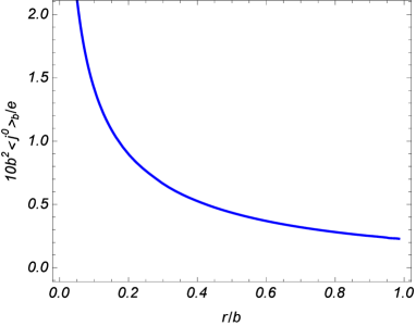
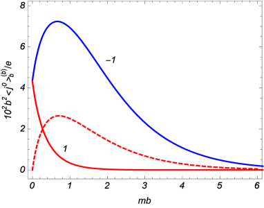
Figure 5: The boundary-induced part in the charge density inside a single boundary with radius $b$ as a function of the radial coordinate (left panel) and of the field mass (right panel) for $\alpha_{0}=1/4$. The left panel is plotted for a massless field. For the right panel $r/b=0.5$ and the numbers near the curves are the values for $s$. The dashed curve presents the charge density in the boundary-free geometry for $s=1$.

As we have mentioned, the last terms in the representations (4.15) and (4.36) are induced when we add the second edge to the geometry with a single boundary. These second boundary-induced contributions are further simplified on the edges $r=a$ and $r=b$ respectively. The corresponding expressions can be written in a combined form

$$\langle j^{0}\rangle=\langle j^{0}\rangle_{u}+\frac{e}{\pi^{2}}\sum_{n=0}^{\infty}\,\sum_{p=\pm}p\int_{m}^{\infty}dx\,\frac{x}{\sqrt{x^{2}-m^{2}}}\mathrm{Re}\left[(sm+i\sqrt{x^{2}-m^{2}})\Omega_{un_{p}}(ax,bx)\right],$$ (4.41)

on the edge $r=u$ with $u=a,b$. The second term in the right-hand side presents the charge induced on the edge $r=u$ by the other edge.

An important point to be mentioned here is that the VEV of the charge density is finite on the edges (note that for the evaluation of the corresponding limiting value of the single boundary-induced parts $\langle j^{0}\rangle_{u}^{\mathrm{(b)}}$, $u=a,b$, we cannot directly put $r=u$ in the representations (4.26) and (4.38) as the separate integrals in the summation over $p$ logarithmically diverge in the upper limit). From the theory of the Casimir effect it is known that in quantum field theory with boundary conditions imposed on the field operator the VEVs of local physical observables, in general, diverge on the boundaries. For example, the latter is the case for the VEV of the energy-momentum tensor or for the fermion condensate in problems with fermionic fields. The appearance of surface divergences in this type of quantities is a consequence of the idealization replacing the physical interaction by the imposition of boundary conditions and indicates that a more realistic physical model should be employed. For example, the microstructure of the boundary on small scales can introduce a physical cutoff needed to produce finite values for surface quantities.

5 Azimuthal current

Now we turn to the spatial components of the fermionic current density. First of all, by using the mode functions (3.12) it is seen that the mode-sum (2.7) for the radial component of the current density vanishes, $\langle j^{1}\rangle=0$, and the only nonzero component corresponds to the azimuthal current. The corresponding mode-sum for the physical component $\langle j_{\phi}\rangle=r\langle j^{2}\rangle$ is presented in the form

$$\langle j_{\phi}\rangle=-\frac{\pi e}{16a^{3}}\sum_{j}\,\sum_{\kappa=\pm}\epsilon_{j}\sum_{l=1}^{\infty}T_{\beta_{j}}^{ab}(\eta,z_{l})h_{2}(z_{l}).$$ (5.1)

with the function

$$h_{2}(z)=z^{2}\frac{g_{\beta_{j},\beta_{j}}(z,zr/a)}{\sqrt{z^{2}/a^{2}+m^{2}}}g_{\beta_{j},\beta_{j}+\epsilon_{j}}(z,zr/a).$$ (5.2)

As before, the terms $\kappa=-$ and $\kappa=+$ are the contributions from the negative- and positive-energy modes.

For the separation of the effects induced by the boundaries we apply to the series over $l$ the summation formula (4.3) with $h(z)=h_{2}(z)$. For the function (5.2) one gets

$$h_{2}(ze^{pi\frac{\pi}{2}})=-\frac{4}{\pi^{2}}\frac{pi\epsilon_{j}z^{2}G_{\beta_{j}}^{(ap)}(z,zr/a)}{\sqrt{(ze^{p\pi i/2})^{2}/a^{2}+m^{2}}}G_{\beta_{j}+\epsilon_{j}}^{(ap)}(z,zr/a).$$ (5.3)

By taking into account Eq. (4.6), we conclude that in the last integral of Eq. (4.3) for the integration range $[0,ma]$ the terms with $p=+$ and $p=-$ cancel each other. For the integration range $[ma,\infty)$ of the remaining integral $\kappa$ and $p$ appear in the form of the product $\kappa p$ and, hence, the negative- and positive-energy modes give the same contribution to the last term. As a consequence, the current density is presented as

$$\langle j_{\phi}\rangle = \langle j_{\phi}\rangle_{a}-\frac{e}{\pi^{2}}\sum_{j}\,\int_{m}^{\infty}dx\,\frac{x^{2}}{\sqrt{x^{2}-m^{2}}}$$ (5.4)

$$\times\mathrm{Re}\left[\Omega_{a\beta_{j}}(ax,bx)G_{\beta_{j}}^{(a)}(ax,rx)G_{\beta_{j}+\epsilon_{j}}^{(a)}(ax,rx)\right],$$

where

$$\langle j_{\phi}\rangle_{a}=-\frac{e}{4\pi a^{3}}\sum_{j}\,\sum_{\kappa=\pm}\int_{0}^{\infty}dx\,\frac{\epsilon_{j}h_{2}(x)}{J_{\beta_{j}}^{(a)2}(x)+Y_{\beta_{j}}^{(a)2}(x)}.$$ (5.5)

The part (5.5) comes from the first term in the right-hand side of the summation formula (4.3). By taking into account that in the limit $b\rightarrow\infty$ the last term in Eq. (5.4) vanishes, we conclude that $\langle j_{\phi}\rangle_{a}$ is the current density in the region $r\geqslant a$ for the geometry with a single boundary at $r=a$.

For the separation of the boundary-induced effects in Eq. (5.5) we use the relation

$$\frac{g_{\beta_{j},\beta_{j}}(z,y)g_{\beta_{j},\beta_{j}+\epsilon_{j}}(z,y)}{J_{\beta_{j}}^{(a)2}(x)+Y_{\beta_{j}}^{(a)2}(x)}=J_{\beta_{j}}(y)J_{\beta_{j}+\epsilon_{j}}(y)-\frac{1}{2}\sum_{l=1,2}\frac{J_{\beta_{j}}^{(a)}(z)}{H_{\beta_{j}}^{(al)}(z)}H_{\beta_{j}}^{(l)}(y)H_{\beta_{j}+\epsilon_{j}}^{(l)}(y).$$ (5.6)

The further transformations are similar to that for the charge density. Substituting Eq. (5.6) into Eq. (5.5), in the part with the last term we rotate the integration contour by the angle $\pi/2$ for the term with $l=1$ and by the angle $-\pi/2$ for the $l=2$ term. The integrals over the intervals $[0,ima]$ and $[0,-ima]$ are canceled. As a result, the contribution (5.5) is presented in the decomposed form

$$\langle j_{\phi}\rangle_{a}=\langle j_{\phi}\rangle_{0}+\langle j_{\phi}\rangle_{a}^{\mathrm{(b)}},$$ (5.7)

where the separate terms are given by the expressions

$$\langle j_{\phi}\rangle_{0}=-\frac{e}{2\pi}\sum_{j}\,\epsilon_{j}\int_{0}^{\infty}dx\,x^{2}\frac{J_{\beta_{j}}(rx)J_{\beta_{j}+\epsilon_{j}}(rx)}{\sqrt{x^{2}+m^{2}}},$$ (5.8)

and

$$\langle j_{\phi}\rangle_{a}^{\mathrm{(b)}}=\frac{e}{\pi^{2}}\sum_{j}\,\int_{m}^{\infty}dx\,\frac{x^{2}}{\sqrt{x^{2}-m^{2}}}\mathrm{Re}\left[\frac{I_{\beta_{j}}^{(a)}(ax)}{K_{\beta_{j}}^{(a)}(ax)}\right]K_{\beta_{j}}(rx)K_{\beta_{j}+\epsilon_{j}}(rx).$$ (5.9)

For $\alpha$ different from a half-odd integer, the part $\langle j_{\phi}\rangle_{a}^{\mathrm{(b)}}$ vanishes in the limit $a\rightarrow 0$ and, hence, in this case Eq. (5.8) is interpreted as the current density in two dimensional space without boundaries. Respectively, the part (5.9) presents the contribution induced in the region $r\leqslant a$ by a single boundary at $r=a$. In the special case $s=1$, the single boundary-induced contribution coincides with the result previously obtained in [22] for a more general geometry of a conical space (with the sign difference explained above).

The boundary-free part in the current density, given by Eq. (5.8), does not depend on the parameter $s$ and, hence, on the irreducible representation of the Clifford algebra in (2+1)-dimensional spacetime. A more convenient expression for this part is provided in Ref. [22]

$$\langle j_{\phi}\rangle_{0}=\frac{e\sin\left(\pi\alpha_{0}\right)}{4\pi^{2}r^{2}}\int_{0}^{\infty}dz\,\frac{\cosh(2\alpha_{0}z)}{\cosh^{3}z}\left(1+2mr\cosh z\right)e^{-2mr\cosh z}.$$ (5.10)

An alternative expression is given in [12]:

$$\langle j_{\phi}\rangle_{0}=-\frac{er}{\pi^{3}}\sin(\pi\alpha_{0})\int_{m}^{\infty}dx\,x^{3}\frac{K_{\alpha_{0}}^{2}(rx)-K_{1-\alpha_{0}}(rx)K_{1+\alpha_{0}}(rx)}{\sqrt{x^{2}-m^{2}}}.$$ (5.11)

Unlike the case of the charge density, the current density does not vanish for a massless field. For a massive field, at distances $mr\gg 1$, it behaves as $e^{-2mr}/r^{3/2}$. At the origin the current density diverges like $1/r^{2}$. Similarly to the case of the charge density in the boundary-free geometry, $\langle j_{\phi}\rangle_{0}$ is discontinuous at half-odd integer values of $\alpha$ with the discontinuity $2\langle j_{\phi}\rangle_{0}|_{\alpha_{0}=1/2}$. In particular, for a massless field for the discontinuity one has $e/(2\pi^{2}r^{2})$.

Decomposing the parameter $\alpha$ in accordance with Eq. (4.14) and redefining the summation variable $j$, the current density is presented in the form

$$\langle j_{\phi}\rangle = \langle j_{\phi}\rangle_{0}+\langle j_{\phi}\rangle_{a}^{\mathrm{(b)}}-\frac{e}{\pi^{2}}\sum_{n=0}^{\infty}\,\sum_{p=\pm}p\,\int_{m}^{\infty}dx\,\frac{x^{2}}{\sqrt{x^{2}-m^{2}}}$$ (5.12)

$$\times\mathrm{Re}\left[\Omega_{an_{p}}(ax,bx)G_{n_{p}}^{(a)}(ax,rx)G_{n_{p}+1}^{(a)}(ax,rx)\right],$$

with the single boundary-induced part

$$\langle j_{\phi}\rangle_{a}^{\mathrm{(b)}}=\frac{e}{\pi^{2}}\sum_{n=0}^{\infty}\,\sum_{p=\pm}p\int_{m}^{\infty}dx\,\frac{x^{2}}{\sqrt{x^{2}-m^{2}}}\mathrm{Re}\left[\frac{I_{n_{p}}^{(a)}(ax)}{K_{n_{p}}^{(a)}(ax)}\right]K_{n_{p}}(rx)K_{n_{p}+1}(rx).$$ (5.13)

This representation explicitly shows that the current density does not depend on the integer part $N$ and is an odd function of the fractional part $\alpha_{0}$. For a massless field and at large distances from the boundary, $r\gg a$, the single boundary-induced contribution (5.13) behaves as $\left(a/r\right)^{4-4|\alpha_{0}|}$, $|\alpha_{0}|<1/2$, with the sign $\mathrm{sgn}(\alpha_{0})\langle j_{\phi}\rangle_{a}^{\mathrm{(b)}}/e<0$. In this limit, the total VEV in the geometry of a single boundary is dominated by the boundary-free part. In the case of a massive field, at distances $r\gg a,m^{-1}$, for the part (5.13) one has the suppression by the factor $e^{-2mr}/r^{3/2}$ and the boundary-induced contribution is of the same order as the boundary-free one.

Both the terms in the right-hand side of Eq. (5.7) are discontinuous at half-odd integer values of the parameter $\alpha$. For the corresponding limiting values one has

$$\lim_{\alpha_{0}\rightarrow\pm 1/2}\langle j_{\phi}\rangle_{0}=-\lim_{\alpha_{0}\rightarrow\pm 1/2}\langle j_{\phi}\rangle_{a}^{\mathrm{(b)}}=\pm\frac{em}{2\pi^{2}r}K_{1}(2mr).$$ (5.14)

Though the separate terms are discontinuous, the total current density in the region $r>a$ for the geometry of a single boundary vanishes in the limits $\alpha_{0}\rightarrow\pm 1/2$ and it is continuous. This is the case for the current density (5.12) in the geometry of the ring as well. It can be checked that the last term in the right-hand side of this formula vanishes for $\alpha_{0}\rightarrow\pm 1/2$. Hence, we conclude that the current density in the ring is a continuous function of the magnetic flux including the points corresponding to the half-odd integer values of the magnetic flux in units of the flux quantum.

In order to clarify the dependence of the current density on the parameters of the problem, let us consider numerical examples. The behavior of the current density in the region $a\leqslant r\leqslant b$ as a function of the radial coordinate and of the parameter $\alpha_{0}$ is presented in figure 6. The left panel is plotted for a massless field and for the magnetic flux parameter $\alpha_{0}=1/4$. In this panel, the numbers near the full curves are the values of the ratio $b/a$ and the dashed curve presents the current density in the geometry of a single boundary at $r=a$. The full curves in the right panel are plotted for $b/a=8$, $r/a=2$, $ma=0.1$ and the numbers near them are the values of the parameter $s$. The dashed curve in the right panel corresponds to the current density for a massless field for the same values of $b/a$ and $r/a$. Similarly to the VEV of the charge density, the current density is finite on the edges. As it has been already emphasized, the current density vanishes for half-odd integer values of the ratio of the magnetic flux to the flux quantum, corresponding to $|\alpha_{0}|=1/2$. The graphs show that the current density is peaked near the inner edge and it decreases with decreasing the width of the ring.

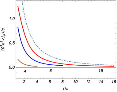
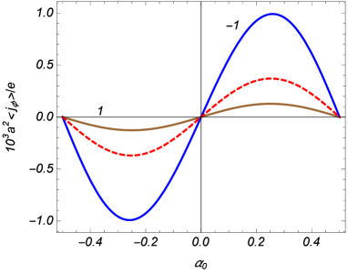
Figure 6: Current density in the region between two boundaries as a function of the radial coordinate for a massless field (left panel) and as a function of the parameter $\alpha_{0}$ (right panel). The left panel is plotted for the magnetic flux parameter $\alpha_{0}=1/4$ and the numbers near the curves are the values of $b/a$. The full curves in the right panel are plotted for $ma=0.1$, $b/a=8$, $r/a=2$ and the numbers near the curves are the values of $s$. The dashed curve in the right panel corresponds to a massless field.

In figure 7, the current density is displayed as a function of the relative location of the outer boundary for fixed values of the parameters $\alpha_{0}=1/4$, $r/a=1.5$. The numbers near the curves are the values for $ma$. The left and right panels correspond to the representations with $s=1$ and $s=-1$, respectively. The dashed lines on both the panels present the current density in the geometry of a single boundary at $r=a$. Again, the graphs show that, for a fixed inner radius, the current density increases with increasing the width of the ring.

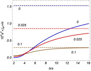
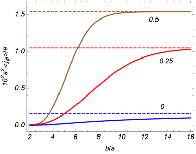
Figure 7: Current density versus the ratio $b/a$ for irreducible representations $s=1$ (left panel) and $s=-1$ (right panel). The graphs are plotted for $\alpha_{0}=1/4$, $r/a=1.5$ and the numbers near the curves are the values of $ma$. The dashed curves present the current density in the geometry of a single boundary at $r=a$.

Similarly to the case of the charge density, we see an essentially different behavior of the current density for the representations $s=1$ and $s=-1$, as a function of the field mass. The dependence of the current density on the mass is plotted in figure 8 for the irreducible representations $s=1$ (left panel) and $s=-1$ (right panel) and for the values of the parameters $\alpha_{0}=1/4$, $b/a=8$, $r/a=2$. The dashed curves present the charge density in the geometry of a single boundary at $r=a$. The dotted line in the right panel is the current density in the boundary-free problem.

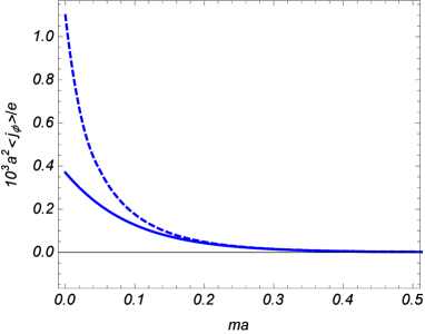
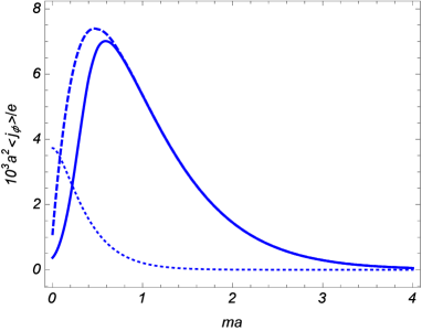
Figure 8: Current density versus the field mass for the fields with $s=1$ (left panel) and $s=-1$ (right panel) and for $\alpha_{0}=1/4$, $b/a=8$, $r/a=2$. The dashed curves present the current density outside a single boundary at $r=a$ and the dotted line is the current density in the boundary-free geometry.

In the representation (5.12) the current density for the geometry of a single boundary at $r=a$ is explicitly separated. The representation with the outer edge contribution separated is obtained by using the identity

$$-\frac{I_{n_{p}}^{(a)}(ax)}{K_{n_{p}}^{(a)}(ax)}K_{n_{p}}(rx)K_{n_{p}+1}(rx)=\frac{K_{n_{p}}^{(b)}(bx)}{I_{n_{p}}^{(b)}\left(bx\right)}I_{n_{p}}\left(rx\right)I_{n_{p}+1}\left(rx\right)$$

$$\qquad+\sum_{u=a,b}n_{u}\Omega_{un_{p}}(ax,bx)G_{n_{p},n_{p}}^{(u)}(ux,rx)G_{n_{p},n_{p}+1}^{(u)}(ux,rx).$$ (5.15)

With this relation, the current density in the region $a\leqslant r\leqslant b$ is presented as

$$\langle j_{\phi}\rangle = \langle j_{\phi}\rangle_{b}-\frac{e}{\pi^{2}}\sum_{n=0}^{\infty}\,\sum_{p=\pm}p\,\int_{m}^{\infty}dx\,\frac{x^{2}}{\sqrt{x^{2}-m^{2}}}$$ (5.16)

$$\times\mathrm{Re}\left[\Omega_{bn_{p}}(ax,bx)G_{n_{p},n_{p}}^{(b)}(bx,rx)G_{n_{p},n_{p}+1}^{(b)}(bx,rx)\right].$$

Here

$$\langle j_{\phi}\rangle_{b}=\langle j_{\phi}\rangle_{0}+\langle j_{\phi}\rangle_{b}^{\mathrm{(b)}},$$ (5.17)

with

$$\langle j_{\phi}\rangle_{b}^{\mathrm{(b)}}=-\frac{e}{\pi^{2}}\sum_{n=0}^{\infty}\,\sum_{p=\pm}p\,\int_{m}^{\infty}dx\,\frac{x^{2}}{\sqrt{x^{2}-m^{2}}}\mathrm{Re}\left[\frac{K_{n_{p}}^{(b)}(bx)}{I_{n_{p}}^{(b)}(bx)}\right]I_{n_{p}}(rx)I_{n_{p}+1}(rx).$$ (5.18)

By taking into account that for $|\alpha_{0}|\neq 1/2$ one has $\Omega_{bn_{p}}(az,bz)\sim a^{2n+1+2\alpha_{0}}$ for $a\rightarrow 0$, from Eq. (5.16) we conclude that the part $\langle j_{\phi}\rangle_{b}$ is the current density in the region $0\leqslant r\leqslant b$ for the geometry of a single boundary at $r=b$ and the contribution (5.18) is induced by the boundary. For points near the center of the disc $r\leqslant b$, the dominant contribution to the edge-induced part (5.18) comes from the term $n=0$ and it behaves as $r^{1-2|\alpha_{0}|}$. By taking into account that the boundary-free part behaves like $1/r^{2}$, we see that near the center the current density is dominated by the boundary-free part.

For the magnetic flux parameter $\alpha_{0}=1/4$, the boundary-induced charge density (5.18) in the geometry of a single boundary at $r=b$ is plotted in figure 9 versus the radial coordinate and the mass. The dashed curve corresponds to the current density in the boundary-free problem. The left panel is plotted for a massless field and the numbers near the curves on the right panel are the values of the parameter $s$ and we have taken $r/b=0.5$.

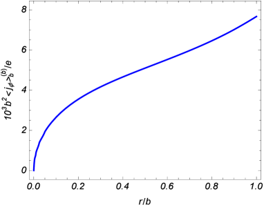
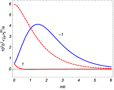
Figure 9: The boundary-induced contribution to the current density inside a single circular boundary with radius $b$ versus the radial coordinate and the mass for $\alpha_{0}=1/4$. The left panel is plotted for a massless field. For the right panel $r/b=0.5$ and the numbers near the curves are the values of $s$.

The last term in Eq. (5.16) is the current density induced in the region $a\leqslant r\leqslant b$ when we add the boundary at $r=a$ to the geometry of the disc with the radius $b$. All the separate terms in the right-hand side of Eq. (5.16) have jumps at half-odd integer values of $\alpha$. However, it can be seen that the total current density is a continuous function of the magnetic flux and it vanishes for $\alpha=N+1/2$. Similar to the case of the charge density, relatively simple expressions for the second edge-induced parts in the representations (5.12) and (5.16) are obtained on the edges $\ r=a$ and $r=b$, respectively. The current density on the edge $r=u$ with $u=a,b$, is presented in the form

$$\langle j_{\phi}\rangle=\langle j_{\phi}\rangle_{u}+\frac{en_{u}}{\pi^{2}}\sum_{n=0}^{\infty}\,\sum_{p=\pm}p\,\int_{m}^{\infty}dx\,\frac{x}{\sqrt{x^{2}-m^{2}}}\mathrm{Re}\left[(sm+i\sqrt{x^{2}-m^{2}})\Omega_{un_{p}}(ax,bx)\right].$$ (5.19)

Comparing with Eq. (4.41), we see that the second edge-induced contribution in the current density on the first edge is equal to the corresponding charge density for the outer edge and has the opposite sign on the inner edge. These relations between the charge and current densities on the ring edges hold for the total VEVs as well. If we formally put $r=a,b$ in the mode sums (4.1) and (5.1), then, by using the Wronskian relation for the Bessel and Neumann functions and Eq. (3.15) for the eigenvalues of the radial quantum number, we can see that

$$\langle j^{0}\rangle_{r=u}=n_{u}\langle j_{\phi}\rangle_{r=u}=-\frac{e}{4\pi a^{2}}\sum_{j}\sum_{l=1}^{\infty}\sum_{\kappa=\pm}\,\kappa T_{\beta_{j}}^{ab}(\eta,z_{l})\frac{E+\kappa sm}{E}z_{l}B_{u}(z_{l}).$$ (5.20)

with $u=a,b$ and

$$B_{a}(x)=1,\;B_{b}(x)=J_{\beta_{j}}^{(a)2}\left(x\right)/J_{\beta_{j}}^{(b)2}\left(xb/a\right).$$ (5.21)

This feature is a consequence of the bag boundary conditions we have imposed on the edges (see also [34]).

In the discussion above for the charge and current densities we have assumed that the fermionic field is in the vacuum state. If the field is in thermal equilibrium at finite temperature, in addition to the vacuum parts we have considered here, the expectation values will receive contributions coming from particles and antiparticles (for finite temperature effects on the fermionic charge and current densities in topologically nontrivial spaces see, e.g., [35]; see also [36] for a recent review of finite temperature field theoretical effects in toroidal topology). For a fermionic field with the chemical potential $\mu$, obeying the condition $|\mu|<m$, the charge and current densities at zero temperature coincide with the VEVs we have investigated above. In the case $|\mu|>m$, the zero temperature expectation values in addition to the VEVs will contain contributions from particles or antiparticles (depending on the sign of the chemical potential) filling the states with the energies $E$ in the range $m\leqslant E\leqslant|\mu|$.

6 Charge and current densities in P- and T-symmetric models with applications to graphene rings

By using the results from the previous sections we can obtain the vacuum densities in the parity and time-reversal symmetric massive fermionic models. In (2+1) dimensions the irreducible representations for the Clifford algebra are realized by $2\times 2$ matrices. In cylindrical coordinates, we can choose the Dirac matrix $\gamma^{2}$ in two inequivalent ways: $\gamma^{2}=\gamma_{(s)}^{2}=-is\gamma^{0}\gamma^{1}/r$, where, as before, $s=\pm 1$. The gamma matrices (2.4), we have used in the discussion above, correspond to the representation with the upper sign. Two sets of Dirac matrices $\gamma_{(s)}^{\mu}=(\gamma^{0},\gamma^{1},\gamma_{(s)}^{2})$ realize two inequivalent irreducible representations of the Clifford algebra. In these representations, the mass term in the Lagrangian density for a two-component spinor field,

$$L_{s}=\bar{\psi}_{(s)}(i\gamma_{(s)}^{\mu}D_{\mu}-m)\psi_{(s)},$$ (6.1)

is not invariant under the $P$- and $T$-transformations. Here we assume that both the fields $\psi_{(s)}$ obey the same boundary conditions

$$\left(1+in_{\mu}\gamma_{(s)}^{\mu}\right)\psi_{(s)}(x)=0,$$ (6.2)

on the circular edges $r=a,b$. In order to recover the $P$- and $T$-invariances, let us consider the combined Lagrangian density $L=\sum_{s=\pm 1}L_{s}$. By appropriate transformations of the fields $\psi_{(-1)}$ and $\psi_{(+1)}$, this Lagrangian is invariant under $P$- and $T$-transformations (in the absence of magnetic fields).

In order to relate the fields $\psi_{(s)}$ to the ones we have considered in the evaluation of the vacuum densities, let us introduce new two-component fields $\psi_{(s)}^{\prime}$ in accordance with $\psi_{(+1)}^{\prime}=\psi_{(+1)}$, $\psi_{(-1)}^{\prime}=\gamma^{0}\gamma^{1}\psi_{(-1)}$. In terms of these fields, the Lagrangian density is presented as

$$L=\sum_{s=\pm 1}\bar{\psi}_{(s)}^{\prime}(i\gamma^{\mu}D_{\mu}-sm)\psi_{(s)}^{\prime},$$ (6.3)

where $\gamma^{\mu}=\gamma_{(+1)}^{\mu}$. From Eq. (6.3) we conclude that the equations for the fields with $s=-1$ and $s=+1$ differ by the sign of the mass term and coincide with Eq. (2.1). From the boundary conditions (6.2) it follows that the fields in Eq. (6.3) obey the conditions

$$\left(1+isn_{\mu}\gamma^{\mu}\right)\psi_{(s)}^{\prime}(x)=0,$$ (6.4)

on $r=a,b$. As it is seen, the field $\psi_{(+1)}^{\prime}$ obeys the condition (2.2), whereas the boundary condition for the field $\psi_{(-1)}^{\prime}$ differs by the sign of the term with the normal to the boundary. As it has been already noticed in [26], this type of condition with the reversed sign is an equally acceptable boundary condition for the Dirac equation. Combining $2$-component spinors $\psi_{+}^{\prime}$ and $\psi_{-}^{\prime}$ in a $4$-component one, $\Psi=(\psi_{+}^{\prime},\psi_{-}^{\prime})^{T}$, and introducing $4\times 4$ Dirac matrices $\gamma_{(4)}^{\mu}=\sigma_{3}\otimes\gamma^{\mu}$, the Lagrangian density (6.3) is rewritten in the form

$$L=\bar{\Psi}(i\gamma_{(4)}^{\mu}D_{\mu}-m)\Psi.$$ (6.5)

In this reducible representation, the boundary conditions (6.4) are combined as

$$\left(1+in_{\mu}\gamma_{(4)}^{\mu}\right)\Psi(x)=0.$$ (6.6)

The latter has the form of the standard MIT bag condition for a 4-component spinor.

By taking into account that $\bar{\psi}_{(s)}\gamma_{(s)}^{\mu}\psi_{(s)}=\bar{\psi}_{(s)}^{\prime}\gamma^{\mu}\psi_{(s)}^{\prime}$, for the total VEV of the current density in the model with the combined Lagrangian $L=\sum_{s=\pm 1}L_{s}$, with $L_{s}$ form (6.1), one gets

$$\langle J^{\mu}\rangle=\sum_{s=\pm 1}\langle\bar{\psi}_{(s)}\gamma_{(s)}^{\mu}\psi_{(s)}\rangle=\sum_{s=\pm 1}\langle\bar{\psi}_{(s)}^{\prime}\gamma^{\mu}\psi_{(s)}^{\prime}\rangle.$$ (6.7)

The charge and current densities for the field $\psi_{(+1)}$ are obtained from the expressions given in the previous sections with $s=1$. In order to find the VEVs for the field $\psi_{(-1)}^{\prime}$, we note that it obeys the field equation (2.1) with $s=-1$ and the boundary condition that differs from Eq. (2.2) by the sign of the term containing the normal to the boundaries. Consequently, the VEV $\langle\bar{\psi}_{(-1)}^{\prime}\gamma^{\mu}\psi_{(-1)}^{\prime}\rangle$ is obtained from the corresponding formulas given above taking $s=-1$ and making the replacement

$$n_{u}\rightarrow-n_{u},\;u=a,b$$ (6.8)

(see Eq. (2.3) for the definition of $n_{u}$). In the final formulas this replacement is made through the definition (4.17) for $f=I,K$. From here we conclude that the expressions for the VEVs $\langle\bar{\psi}_{(s)}^{\prime}\gamma^{\mu}\psi_{(s)}^{\prime}\rangle$, $\mu=0,2$, are given by the formulas in sections 4 and 5 where now we should take

$$f_{n_{p}}^{(u)}(z)=\delta_{f}zf_{n_{p}+1}\left(z\right)+n_{u}(m_{u}+si\sqrt{z^{2}-m_{u}^{2}})f_{n_{p}}\left(z\right),$$ (6.9)

with $n_{u}$ defined in accordance with Eq. (2.3). This shows that one has the relation $f_{n_{p}}^{(u)}(z)|_{s=-1}=f_{n_{p}}^{(u)\ast}(z)|_{s=1}$ and, hence, the same for the functions $\Omega_{un_{p}}(ax,bx)$ and $G_{n_{p},\mu}^{(u)}(ux,rx)$. Here the star stands for the complex conjugate. Assuming that the masses $m$ for the fields with $s=+1$ and $s=-1$ are the same, we can see that the boundary-induced contributions from these fields to the charge density cancel each other. By taking into account that the same is the case for the boundary-free part (see Eq. (4.32)), we conclude that the VEV of the total charge density vanishes. For the VEV of the current density, the contributions from the fields $\psi_{(+1)}^{\prime}$ and $\psi_{(-1)}^{\prime}$ coincide for both the boundary-free and boundary-induced parts. The corresponding expressions for the total current (6.7) are obtained from those in the previous section for the case $s=1$ with an additional factor 2. Now, for the field $\psi_{(s)}^{\prime}$ the analog of the relation (5.20) between the charge and current densities on the edges has the form

$$\langle j_{\phi}^{\prime}\rangle_{r=u}=-n_{u}\langle j^{0\prime}\rangle_{r=u},$$ (6.10)

where $\langle j^{\mu\prime}\rangle=\langle\bar{\psi}_{(-1)}^{\prime}\gamma^{\mu}\psi_{(-1)}^{\prime}\rangle$, $u=a,b$, and $n_{u}$ is the same as in Eq. (5.20).

Note that we could consider another class of $P$- and $T$-invariant models with two-components fields $\psi_{(s)}$ obeying the boundary conditions in which the sign of the term in Eq. (6.2), containing the normal vector, is reversed. For these models, the same reversion should be made in the boundary condition (6.4) for the primed fields. Now we see that the charge and current densities for the field $\psi_{(-1)}^{\prime}$ coincide with those in the previous sections for $s=-1$, whereas the results for the field $\psi_{(+1)}^{\prime}$ are obtained from those before in the case $s=1$ by the replacement (6.8). The total charge density, combined from the fields with $s=1$ and $s=-1$ vanishes as in the previous case, and the current density is obtained from the expressions in section 5 in the case $s=-1$ with the additional factor 2. As we have seen, in this case the dependence of the VEV on the field mass is more interesting. Of course, there is another possibility when the boundary conditions for the fields $\psi_{(s)}$ are different for $s=1$ and $s=-1$. For example, we could impose the condition (6.2) with the additional factor $s$ in the term involving the normal vector. In this case the primed fields will obey the same boundary condition (Eq. (6.4) with $s=1$) and the corresponding VEVs exactly coincide with those in sections 4 and 5. In this variant, there is no cancellation and the total charge density does not vanish.

The field theoretical models we have considered can be realized by various graphene made structures. For example, the geometry with a single boundary at $r=a$ corresponds to a circular graphene dot if the region $r<a$ is considered and to a single circular nanohorn (or nanopore) for the region $r>a$. The influence of boundaries on the electronic properties of a circular graphene quantum dot in a magnetic field has been discussed in [37]. Comparing the analytical results obtained within the continuum model to those obtained from the tight-binding model, the authors conclude that the Dirac model with the infinite-mass boundary condition describes rather well its tight-binding analog and is in good qualitative agreement with experiments. Considering different boundary conditions in the Dirac model for graphene devices, a similar conclusion is made in Ref. [34]. The Aharonov-Bohm effect and persistent currents in graphene nanorings have been recently investigated in [29, 38]. The effect of impurity on persistent currents in strictly one-dimensional Dirac systems is discussed in [39].

The results obtained above can be applied for the investigation of the ground state charge and current densities in graphene rings. Graphene is a monolayer of carbon atoms with honeycomb lattice containing two triangular sublattices $A$ and $B$ related by inversion symmetry. The electronic subsystem in a graphene sheet is among the most popular realizations of the Dirac physics in two spatial dimensions (for other planar condensed-matter systems with the low-energy excitations described by the Dirac model see Ref. [40]). For a given value of spin $S=\pm 1$, the corresponding long wavelength excitations are described in terms of 4-component spinors $\Psi_{S}=(\psi_{+,AS},\psi_{+,BS},\psi_{-,AS},\psi_{-,BS})^{T}$ with the Lagrangian density (in the standard units)

$$L=\sum_{S=\pm 1}\bar{\Psi}_{S}(i\hbar\gamma^{0}\partial_{t}+i\hbar v_{F}\gamma^{l}D_{l}-\Delta)\Psi_{S}.$$ (6.11)

Here, $D_{l}=(\mathbf{\nabla}-ie\mathbf{A}/\hbar c)_{l}$, $l=1,2$, is the spatial part of the gauge extended covariant derivative and $e=-|e|$ for electrons. The Fermi velocity $v_{F}$ plays the role of the speed of light. It is expressed in terms of the microscopic parameters as $v_{F}=\sqrt{3}a_{0}\gamma_{0}/(2\hbar)\approx 7.9\times 10^{7}$ cm/s, where $a_{0}\approx 1.42$ Å is the inter-atomic spacing of graphene honeycomb lattice and $\gamma_{0}\approx 2.9$ eV is the transfer integral between first-neighbor $\pi$ orbitals. The components $\psi_{\pm,AS}$ and $\psi_{\pm,BS}$ of the spinor $\Psi_{S}$ give the amplitude of the electron wave function on sublattices $A$ and $B$. The indices $+$ and $-$ of these components correspond to inequivalent points, $\mathbf{K}_{+}$ and $\mathbf{K}_{-}$, at the corners of the two-dimensional Brillouin zone (see Ref. [2]). The energy gap $\Delta$ in Eq. (6.11) is related to the corresponding Dirac mass as $\Delta=mv_{F}^{2}$. It plays an important role in many physical applications (for the mechanisms of the gap generation in the energy spectrum of graphene see, for example, Ref. [2] and references therein). Depending of the physical mechanism for the generation, the energy gap may take values in the range $1\,\mathrm{meV}\lesssim\Delta\lesssim 1\,\mathrm{eV}$.

Comparing with the discussion above, we see that the values of the parameter $s=+1$ and $s=-1$ correspond to the $\mathbf{K}_{+}$ and $\mathbf{K}_{-}$ points of the graphene Brillouin zone and the Lagrangian density (6.11) is the analog of (6.5). From here we conclude that, for a given value of the spin $S$, the expressions for the VEVs of the charge and current densities for separate contributions coming from the points $\mathbf{K}_{+}$ and $\mathbf{K}_{-}$ are obtained from the formulas in previous sections by the replacement $m\rightarrow a_{0}^{-1}\Delta/\gamma_{F}$, where $\gamma_{F}=\hbar v_{F}/a_{0}\approx 2.51$ eV determines the energy scale in the model. In the expressions for the current density, an additional factor $v_{F}$ should be added, because now the operator of the spatial components of the current density is defined as $j^{\mu}=ev_{F}\bar{\psi}(x)\gamma^{\mu}\psi(x)$, $\mu=1,2$. For a given spin $S$, the contributions from two valleys are combined in accordance with Eq. (6.7). In the problem at hand, the spins $S=\pm 1$ give the same contributions to the total VEVs. As it has been mentioned before, the charge density vanishes as a result of cancellation of the contributions from the $\mathbf{K}_{+}$ and $\mathbf{K}_{-}$ points. The effective charge density may appear if the gap generation mechanism breaks the valley symmetry and the mass gap is different for $s=+1$ and $s=-1$. Note that this will break $P$- and $T$-invariances of the model.

7 Summary

In both the field theoretical and condensed matters aspects, among the most interesting topics in quantum field theory is the investigation of the effects induced by gauge field fluxes on the properties of the quantum vacuum. In the present paper we have discussed the combined effects from the magnetic flux and boundaries on the VEVs of the fermionic charge and current densities in a two-dimensional circular ring. The examples of graphene nanoriboons and rings have already shown that the edge effects have important consequences on the physical properties of planar systems. In the problem at hand, for the field operator on the ring edges we have imposed the bag boundary conditions. The distribution of the magnetic flux inside the inner edge can be arbitrary. The boundary separating the ring from the region of the location for the gauge field strength is impenetrable for the fermionic field and the effect of the gauge field is purely topological. It depends on the total flux alone. The latter gives rise the Aharonov-Bohm effect for physical characteristics of the ground state. The consideration is done for both irreducible representations of the Clifford algebra in (2+1) dimensions. In these representations the mass term in the Dirac equation breaks the parity and time-reversal invariances. For the evaluation of the VEVs we have employed the method based on the direct summation over a complete set of fermionic modes in the ring. The corresponding positive- and negative-energy wavefunctions are given by Eq. (3.12) with the radial functions defined by Eq. (3.13). The eigenvalues of the radial quantum number are quantized by the boundary conditions and are roots of the equation (3.15). The eigenvalue equations for the positive- and negative-energy modes differ by the sign of the energy. Alternatively, we can take the negative-energy modes in the form (3.21). With this representation, the eigenvalue equation for the negative-energy modes is obtained from the positive-energy one by inverting the sign of the parameter $\alpha$, the latter being the ratio of the magnetic flux to the flux quantum.

The mode-sums for VEVs of the charge and current densities, Eqs. (4.1) and (5.1), contain series over the roots of Eq. (3.15). The latter are given implicitly and these representations are not well adapted for the investigation of the VEVs. More convenient expressions are obtained by making use of the generalized Abel-Plana formula (4.3) for the summation of the series. The formulas obtained in this way have two important advantages: the explicit knowledge of the eigenvalues is not required and the boundary-induced contributions to the VEVs are explicitly extracted. In addition, instead of series with highly oscillatory terms for large values of quantum numbers, in the new representation one has exponentially convergent integrals for points away from the edges. This is an important point from the point of view of numerical evaluations.

The VEVs for both the charge and current densities are decomposed into boundary-free, single boundary-induced and the second boundary-induced contributions. All them are odd periodic functions of the magnetic flux with the period equal to the flux quantum. For the geometry with two boundaries we have provided two representations, given by Eqs. (4.15) and (4.36) for the charge and by Eqs. (5.12) and (5.16) for the azimuthal current. In these representations the contributions for the exterior or interior geometries with a single boundary are explicitly extracted. The last terms in all the representations are induced by the introduction of the second boundary to the geometry with a single boundary. The single boundary parts in the VEVs are given by the expressions (4.21) and (5.13) in the exterior region and by Eqs. (4.38) and (5.18) for the interior region.

Unlike the case of the boundary-free geometry the charge and current densities in the ring are continuous at half-odd integer values for the ratio of the magnetic flux to the flux quantum, and both of them vanish at these points. We have shown that the behaviour of the VEVs as functions of the field mass (energy gap in field theoretical models of planar condensed matter system) is essentially different for the cases $s=1$ and $s=-1$. With the initial increase of the mass from the zero value, the modulus for the charge and current densities decreases for the irreducible representation with $s=1$ and increases for the one with $s=-1$. With further increase of the mass the vacuum densities are suppressed in both cases. An important feature that distinguishes the VEVs of the charge and current densities from those for the energy-momentum tensor is their finiteness on the boundaries. On the outer edge the current density is equal to the charge density whereas on the inner edge they have opposite signs. For a fixed values of the other parameters, both the charge and current densities decrease by the modulus with decreasing outer radius.

The boundary condition (2.2) we have considered contains no additional parameters and is a special case in a general class of boundary conditions for the Dirac equation confining the fermionic field in a finite volume. It is the most popular boundary condition in the investigations of the fermionic Casimir effect for various types of the bulk and boundary geometries. On the base of the analysis given above we can consider another boundary condition that differs from (2.2) by the sign of the term containing the normal to the boundary. The corresponding expressions for the VEVs of the charge and current densities are obtained from those in sections 4 and 5 by making the replacement (6.8) for $n_{u}$ defined by Eq. (2.3). All the final formulas (for example, Eqs. (4.15), (5.16)) remain the same with the only difference in the definition of the notation (4.17), where now $n_{u}$ should be replaced by $-n_{u}$. Equivalently, the results for the field with a given $s$ and with the modified boundary condition are obtained from the corresponding expressions for the field with $-s$ and obeying the condition (2.2) replacing $f_{n_{p}}^{(u)}(z)$ by its complex conjugate, $f_{n_{p}}^{(u)\ast}(z)$. With the modified boundary condition, the current density is equal to the charge density on the inner edge and has the opposite sign on the outer edge.

The charge and current densities in parity and time-reversal models are obtained combining the results for the separate cases with $s=1$ and $s=-1$. These models can be formulated in terms of four-component spinors constructed from the 2-component spinors realizing the two different irreducible representations. Assuming that both these spinors obey the boundary condition (2.2) and have the same mass, the resulting charge density vanishes, whereas the current density is obtained from the expressions given in section 5 with the additional factor 2. For the graphene circular rings, an additional factor 2 comes from the spin degree of freedom.

References

- [1] E. Fradkin, Field Theories of Condensed Matter Systems (Addison-Wesley Publishing Company, Reading, 1991); Y. Imry, Introduction to Mesoscopic Physics (Oxford University Press, Oxford, 1997); G.V. Dunne, Topological Aspects of Low Dimensional Systems (Springer, Berlin, 1999); Xiao-Liang Qi and Shou-Cheng Zhang, Rev. Mod. Phys. 83, 1057 (2011).
- [2] V.P. Gusynin, S.G. Sharapov, and J.P. Carbotte, Int. J. Mod. Phys. B 21, 4611 (2007); A.H. Castro Neto, F. Guinea, N.M.R. Peres, K.S. Novoselov, and A.K. Geim, Rev. Mod. Phys. 81, 109 (2009); M.A.H. Vozmediano, M.I. Katsnelson, and F. Guinea, Phys. Rep. 496, 109 (2010).
- [3] S. Deser, R. Jackiw, and S. Templeton, Ann. Phys. (N.Y.) 140, 372 (1982).
- [4] A.J. Niemi and G.W. Semenoff, Phys. Rev. Lett. 51, 2077 (1983).
- [5] P. Cea, Phys. Rev. D 34, 3229 (1986).
- [6] Y. Hosotani, Phys. Lett. B 319, 332 (1993); Y. Hosotani, Phys. Rev. D 51, 2022 (1995); D. Cangemi, E. D’Hoker, and G. Dunne, Phys. Rev. D 51, 2513 (1995); D. Wesolowski and Y. Hosotani, Phys. Lett. B 354, 396 (1995); T. Itoh and T. Sato, Phys. Lett. B 367, 290 (1996); P. Cea, Phys. Rev. D 55, 7985 (1997).
- [7] K.G. Klimenko, Z. Phys. C 54, 323 (1992); K.G. Klimenko, Theor. Math. Phys. 90, 1 (1992).
- [8] V.P. Gusynin, V.A. Miransky and L.A. Shovkovy, Phys. Rev. D 52, 4718 (1995); R.R. Parwani, Phys. Lett. B 358, 101 (1995); G. Dunne and T. Hall, Phys. Rev. D 53, 2220 (1996); A. Das and M. Hott, Phys. Rev. D 53, 2252 (1996); M. de J. Anguiano-Galicia, A. Bashir, and A. Raya, Phys. Rev. D 76, 127702 (2007); A. Raya and E. Reyes, Phys. Rev. D 82, 016004 (2010).
- [9] A.N. Redlich, Phys. Rev. D 29, 2366 (1984); R. Jackiw, Phys. Rev. D 29, 2375 (1984); D. Boyanovsky and R. Blankenbecler, Phys. Rev. D 31, 3234 (1985); R. Blankenbecler and D. Boyanovsky, Phys. Rev. D 34, 612 (1986); A.P. Polychronakos, Nucl. Phys. B 278, 207 (1986).
- [10] T. Jaroszewicz, Phys. Rev. D 34, 3128 (1986).
- [11] P. Górnicki, Ann. Phys. (N.Y.) 202, 271 (1990).
- [12] E.G. Flekkøy and J.M. Leinaas, Int. J. Mod. Phys. A 6, 5327 (1991).
- [13] H. Li, D.A. Coker, and A.S. Goldhaber, Phys. Rev. D 47, 694 (1993); V.B. Bezerra and E.R. Bezerra de Mello, Class. Qiantum Grav. 11, 457 (1994); E.R. Bezerra de Mello, Class. Qiantum Grav. 11, 1415 (1994); Yu.A. Sitenko, Phys. Rev. D 60, 125017 (1999); R. Jackiw, A.I. Milstein, S.-Y. Pi, and I.S. Terekhov, Phys. Rev. B 80, 033413 (2009); A.I. Milstein and I.S. Terekhov, Phys. Rev. B 83, 075420 (2011).
- [14] C.W.J. Beenakker, Rev. Mod. Phys. 80, 1337 (2008); K. Wakabayashi, S. Dutta, Solid State Commun. 152, 1420 (2012).
- [15] V.M. Mostepanenko, N.N. Trunov, The Casimir Effect and Its Applications (Clarendon, Oxford, 1997); K.A. Milton, The Casimir Effect: Physical Manifestation of Zero-Point Energy (World Scientific, Singapore, 2002); V.A. Parsegian, Van der Waals Forces (Cambridge University Press, Cambridge, 2005); M. Bordag, G.L. Klimchitskaya, U. Mohideen, and V.M. Mostepanenko, Advances in the Casimir Effect (Oxford University Press, Oxford, 2009); Casimir Physics, edited by D. Dalvit, P. Milonni, D. Roberts, and F. da Rosa, Lecture Notes in Physics Vol. 834 (Springer-Verlag, Berlin, 2011).
- [16] G.L. Klimchitskaya, U. Mohidden, and V.M. Mostepanenko, Rev. Mod. Phys. 81, 1827 (2009).
- [17] S. Bellucci and A.A. Saharian, Phys. Rev. D 79, 085019 (2009); S. Bellucci, A.A. Saharian, and V.M. Bardeghyan, Phys. Rev. D 82, 065011 (2010).
- [18] S. Bellucci, A.A. Saharian, and H.A. Nersisyan, Phys. Rev. D 88, 024028 (2013).
- [19] E.R. Bezerra de Mello, A.A. Saharian, and V. Vardanyan, Phys. Lett. B 741, 155 (2015).
- [20] S. Bellucci and A.A. Saharian, Phys. Rev. D 87, 025005 (2013); S. Bellucci, A.A. Saharian, and N.A. Saharyan, Eur. Phys. J. C 75, 378 (2015).
- [21] S. Bellucci, A.A. Saharian, and V. Vardanyan, JHEP 11 (2015) 092; S. Bellucci, A.A. Saharian, and V. Vardanyan, Phys. Rev. D 93, 084011 (2016).
- [22] E. R. Bezerra de Mello, V. Bezerra, A.A. Saharian, and V.M. Bardeghyan, Phys. Rev. D 82, 085033 (2010).
- [23] E.R. Bezerra de Mello, V.B. Bezerra, A.A. Saharian, and H.H. Harutyunyan, Phys. Rev. D 91, 064034 (2015).
- [24] S. Leseduarte and A. Romeo, Commun. Math. Phys. 193, 317 (1998); C.G. Beneventano, M. De Francia, K. Kirsten, and E.M. Santangelo, Phys. Rev. D 61, 085019 (2000); M. De Francia and K. Kirsten, Phys. Rev. D 64, 065021 (2001).
- [25] A. Chodos, R. Jaffe, K. Johnson, C. Thorn, and V. Weisskopf, Phys. Rev. D 9, 3741 (1974); K. Johnson, Acta Phys. Pol. B 6, 865 (1975).
- [26] M.V. Berry and R.J. Mondragon, Proc. R. Soc. London, Ser. A 412, 53 (1987).
- [27] E. McCann and V. I. Fal’ko, J. Phys.: Condens. Matter 16, 2371 (2004); A.R. Akhmerov and C.W.J. Beenakker, Phys. Rev. Lett. 98, 157003 (2007); A.R. Akhmerov and C.W.J. Beenakker, Phys. Rev. B 77, 085423 (2008); J.A.M. van Ostaay, A.R. Akhmerov, C.W.J. Beenakker, and M. Wimmer, Phys. Rev. B 84, 195434 (2011); Yu.A. Sitenko, Phys. Rev. D 91, 085012 (2015).
- [28] A.A. Saharian, The Generalized Abel-Plana Formula with Applications to Bessel Functions and Casimir Effect (Yerevan State University Publishing House, Yerevan, 2008); Preprint ICTP/2007/082; arXiv:0708.1187.
- [29] P. Recher, B. Trauzettel, A. Rycerz, Y.M. Blanter, C.W.J. Beenakker, and A.F. Morpurgo, Phys. Rev. B 76, 235404 (2007).
- [30] A.P. Prudnikov, Yu.A. Brychkov, and O.I. Marichev, Integrals and Series (Gordon and Breach, New York, 1986), Vol. 2.
- [31] E.R. Bezerra de Mello and A.A. Saharian, Class. Quantum Grav. 23, 4673 (2006).
- [32] P. de Sousa Gerbert and R. Jackiw, Commun. Math. Phys. 124, 229 (1989); P. de Sousa Gerbert, Phys. Rev. D 40, 1346 (1989); Yu.A. Sitenko, Ann. Phys. (N.Y.) 282, 167 (2000).
- [33] C.R. Hagen, Phys. Rev. Lett. 64, 503 (1990); C.R. Hagen, Int. J. Mod. Phys. A 6, 3119 (1991); C.R. Hagen, Phys. Rev. D 48, 5935 (1993); M. Bordag and S. Voropaev, J. Phys A: Math. Gen. 26, 1631 (1993); M. Bordag and S. Voropaev, Phys. Lett. B 333, 238 (1994); C.R. Hagen and D.K. Park, Ann. Phys. (N.Y.) 251, 45 (1996); J. Spinelly and E.R. Bezerra de Mello, Class. Quantum Grav. 20, 873 (2003); F.M. Andrade, E.O. Silva, and M. Pereira, Phys. Rev. D 85, 041701(R) (2012).
- [34] C.G. Beneventano and E.M. Santangelo, Int. J. Mod. Phys.: Conf. Series 14, 240 (2012).
- [35] S. Bellucci, E.R. Bezerra de Mello, and A.A. Saharian, Phys. Rev. D 89, 085002 (2014); A. Mohammadi, E.R. Bezerra de Mello, and A.A. Saharian, J. Phys. A: Math. Theor. 48, 185401 (2015); S. Bellucci, E.R. Bezerra de Mello, E. Bragança, and A.A. Saharian, Eur. Phys. J. C 76, 359 (2016).
- [36] F.C. Khanna, A.P.C. Malbouisson, J.M.C. Malbouisson, and A.E. Santana, Phys. Rep. 539, 135 (2014).
- [37] S. Schnez, K. Ensslin, M. Sigrist, and T. Ihn, Phys. Rev. B 78, 195427 (2008); M. Grujić, M. Zarenia, A. Chaves, M. Tadić, G.A. Farias, and F.M. Peeters, Phys. Rev. B 84, 205441 (2011).
- [38] C.-H. Yan and L.-F. Wei, J. Phys. Condens. Matter 22, 295503 (2010); J. Wurm, M. Wimmer, H. U. Baranger, and K. Richter, Semicond. Sci. Technol. 25, 034003 (2010); M. M. Ma and J. W. Ding, Solid State Commun. 150, 1196 (2010); M. Zarenia, J. Milton Pereira, A. Chaves, F.M. Peeters, and G. A. Farias, Phys. Rev. B 81, 045431 (2010); J. Schelter, P. Recher, and B. Trauzettel, Solid State Commun. 152, 1411 (2012); I. Romanovsky, C. Yannouleas, and U. Landman, Phys. Rev. B 85, 165434 (2012); D. Faria, A. Latgé, S. E. Ulloa, and N. Sandler, Phys. Rev. B 87, 241403(R) (2013).
- [39] D. Sticlet, B. Dóra, and J. Cayssol, Phys. Rev. B 88, 205401 (2013).
- [40] V.P. Gusynin and S.G. Sharapov, Phys. Rev. B 73, 245411 (2006); O. Vafek and A. Vishwanath, Annu. Rev. Condens. Matter Phys. 5, 83 (2014).