YITP-16-44
KIAS-P16060

Mass Deformed ABJM Theory on Three Sphere
in Large $N$ limit


Tomoki Nosaka¹, Kazuma Shimizu² and Seiji Terashima<sup>2


1</sup>: Korea Institute for Advanced Study, Seoul 02455, Korea
²: Yukawa Institute for Theoretical Physics, Kyoto University, Kyoto 606-8502, Japan

In this paper the free energy of the mass deformed ABJM theory on $S^{3}$ in the large $N$ limit is studied. We find a new solution of the large $N$ saddle point equation which exists for an arbitrary value of the mass parameter, and compute the free energies for these solutions. We also show that the solution corresponding to an asymptotically $\text{AdS}_{4}$ geometry is singular at a certain value of the mass parameter and does not exist over this critical value. It is not clear what the gravity dual of the mass deformed ABJM theory on $S^{3}$ for the mass parameter larger than the critical value is.

1 Introduction

The mass deformed ABJM theory [1, 2, 3] is the theory obtained by deforming the three dimensional $U(N)_{k}\times U(N)_{-k}$ ${\cal N}=6$ superconformal Chern-Simons theory (called the ABJM theory) [4] with a set of relevant operators including mass terms for the bi-fundamental chiral multiplets. While the ABJM theory describes the stack of $N$ M2-branes, the mass deformed ABJM theory is expected to describe the bound states of the M2-branes and the M5-branes through the fuzzy sphere configuration given in [5, 3]. This theory has special features which make it worth studying. One of them is that the theory has the ${\cal N}=6$ supersymmetry, which is the (almost) maximum amount of the supersymmetries in three dimension. Nevertheless this theory is not conformal, hence has non-trivial dynamics and a renormalization group flow. Furthermore, in the large $N$ limit this theory will have a gravity dual which should be obtained by a deformation to the gravity dual of the ABJM theory corresponding to the mass terms. Therefore, this theory will be one of the basic models to be investigated in the large $N$ limit.

To study a supersymmetric field theory, we can use the localization technique [7, 8, 9] which enables us to obtain the exact partition function as well as some supersymmetric correlators. Each of these results is, however, given typically by a matrix model, i.e. an integration over the $N\times N$ matrix variables. It is highly non-trivial to take the large $N$ limit in these matrix models.

In this paper, as in our previous work [10], we continue to study the partition function $Z$ of the mass deformed ABJM theory on $S^{3}$ in the large $N$ limit. We find a new solution of the large $N$ saddle point equation with an arbitrary mass parameter and compute the free energy $F\sim N^{2}$ for the solution. We also generalize the ansatz to obtain the free energy $F\sim N^{3/2}$ [10] in full extent, and find that the saddle point solution can not exist for the mass parameter larger than a certain critical value. Because the classical supergravity on an asymptotically $\text{AdS}_{4}$ spacetime has $F\sim N^{3/2}$, there would be no gravity duals for the mass deformed ABJM theory on $S^{3}$ with the mass parameter larger than the critical value.

This result seems surprising, as the critical mass is reached by a finite and relevant deformation from the ABJM theory. Nevertheless, we can argue that this phase transition indeed occurs. If the dimensionless mass parameter $m$, which is the mass parameter normalized by the radius of $S^{3}$, is small enough, the free energy $F$ will behave as $F\sim N^{\frac{3}{2}}$ since the theory reduces to the ABJM theory in the limit $m\rightarrow 0$. The factor $N^{\frac{3}{2}}$ can be interpreted as $1/G_{N}$, hence this free energy is consistent with the classical supergravity. On the other hand, if $m$ is sufficiently large we can integrate out the bi-fundamental hypermultiplets first in the computation of the partition function. As a result we will obtain $F\sim N^{2}$. Indeed, for the new solution we find the free energy scales like $F\sim N^{2}$ (see (3.5) and (3.18)). Therefore, it is possible to have a phase transition in the interpolating regime. The phase transition may be similar to the confinement/deconfinement transition if we regard the change of the mass parameter as a renormalization group flow. We will discuss this aspect in [13].

Note that this phase transition is absent in the ${\cal N}=2^{*}$ supersymmetric Yang-Mills theories on $S^{4}$ which is a four dimensional analogue of the mass deformed ABJM theory. For this theory in the strong ’t Hooft coupling limit the saddle point solution and the free energy are smooth under the change of the mass parameter [14, 15]. Indeed, the free energy of the ${\cal N}=4$ supersymmetric Yang-Mills theory, which is the massless limit of the theory, is $F\sim N^{2}$ also, thus both of the massless and the infinite mass limits are consistent with the gravity duals and can be smoothly connected.

Needless to say, further investigations of the phase transition are desirable. In particular, we should study the vacuum solution in the supergravity corresponding to the mass deformed ABJM theory on $S^{3}$ with an arbitrary mass parameter. We also expect that this kind of phase transition will occur also in the other theories on $S^{3}$ describing the M2-branes in various backgrounds such as [16, 2, 17, 18]. We hope to report on these in near future.

This paper is organized as follows. In the next section we introduce the partition function of the mass deformed ABJM theory which is expressed as a $2N$ dimensional integration. We also write down the saddle point equations to evaluate the large $N$ limit of the partition function. In section 3 and section 4 we solve the saddle point equations and determine the free energy $F=-\log Z$, in the large $N$ limit for various values of the mass deformation parameter. In section 3 we consider the problem in the limit $N\rightarrow\infty$ with $k$ kept finite. In section 4 we take the ’t Hooft limit $k,N\rightarrow\infty$ with $k/N$ finite. In both sections we also evaluate the vacuum expectation values of the $1/6$ BPS Wilson loops for the saddle point configurations and argue the interpretation of our results. Section 5 is devoted for discussion and comments on future directions. In appendix A we comment on another solution to the saddle point equations for finite $k$. This solution give the free energy which is larger than that obtained in the same parameter regime in section 3. Appendix B contains the computation of the ${\cal O}(1/N)$ corrections in the saddle point equations in section 3.1 and 3.2.1, which are though irrelevant to the large $N$ free energy. In appendix C, we rederive the solution which has the gravity dual in a similar way in [10].

2 Saddle point approximation of free energy

As in [10], we will consider the mass deformed ABJM theory which is the 3d ${\cal N}=6$ $U(N)_{k}\times U(N)_{-k}$ SUSY Chern-Simons matter theory with the Chern-Simons level $\pm k$ deformed by the mass terms and the interaction terms which preserve the ${\cal N}=6$ supersymmetry. The action of this theory on $S^{3}$ can be written as

$$S_{\text{mABJM}}=S_{\text{ABJM}}+\frac{i\zeta}{2\pi}\int_{S^{3}}dx^{3}\sqrt{g}\bigl{[}\operatorname{Tr}(D-\sigma)+\operatorname{Tr}({\widetilde{D}}-{\widetilde{\sigma}})\bigr{]},$$ (2.1)

where $(\sigma,D$) are the auxiliary component fields in the $U(N)_{k}$ vector multiplet $(A_{\mu},\sigma,\lambda_{\alpha},D)$, and $({\widetilde{\sigma}},{\widetilde{D}})$ those in $U(N)_{-k}$ vector multiplet (see e.g. eq(3.23) in [19]). Here $\zeta$ is a real parameter which is related to the mass of the matter fields as $m=r_{S^{3}}^{-1}\cdot\zeta/k$.

The supersymmetric gauge theories on the three sphere were studied in [20, 21, 22, 19], with the help of the localization technique. For the mass deformed ABJM theory, it was found that the partition function is given by the following $2N$ dimensional integration

$$Z=\prod_{i=1}^{N}\int d\lambda_{i}d{\widetilde{\lambda}}_{i}e^{-f(\lambda,{\widetilde{\lambda}})},$$ (2.2)

where

$$f(\lambda,{\widetilde{\lambda}}) =\pi ik\sum_{i=1}^{N}(\lambda_{i}^{2}-{\widetilde{\lambda}}_{i}^{2})-2\pi i\zeta\sum_{i=1}^{N}(\lambda_{i}+{\widetilde{\lambda}}_{i})$$

$$\quad-\sum_{\begin{subarray}{c}i,j=1\\ (i>j)\end{subarray}}^{N}\log\sinh^{2}\pi(\lambda_{i}-\lambda_{j})-\sum_{\begin{subarray}{c}i,j=1\\ (i>j)\end{subarray}}^{N}\log\sinh^{2}\pi({\widetilde{\lambda}}_{i}-{\widetilde{\lambda}}_{j})+\sum_{i,j=1}^{N}\log\cosh^{2}\pi(\lambda_{i}-{\widetilde{\lambda}_{j}}).$$ (2.3)

Here $\lambda_{i}$ and ${\widetilde{\lambda}}_{i}$ $(i=1,\ldots,N)$ respectively denote the eigenvalues of the scalar component field in the vector multiplet for $U(N)_{k}$ and those for $U(N)_{-k}$, which are real constant numbers characterizing the saddle point configurations of the fields in the localization computation as

$$\sigma=-D=\begin{pmatrix}\lambda_{1}&&&\\ &\lambda_{2}&&\\ &&\ddots&\\ &&&\lambda_{N}\end{pmatrix},\quad{\widetilde{\sigma}}=-{\widetilde{D}}=\begin{pmatrix}{\widetilde{\lambda}}_{1}&&&\\ &{\widetilde{\lambda}}_{2}&&\\ &&\ddots&\\ &&&{\widetilde{\lambda}}_{N}\end{pmatrix},\quad\text{(other fields)}=0.$$ (2.4)

In the limit of $N\rightarrow\infty$, these $2N$ integrations can be evaluated by using the saddle point approximation

$$Z\approx e^{-f(\lambda,{\widetilde{\lambda}})},$$ (2.5)

with the eigenvalues $(\lambda,{\widetilde{\lambda}})$ being solutions to the following saddle point equations

$$0 =\frac{\partial f(\lambda,{\widetilde{\lambda}})}{\partial\lambda_{i}}=2\pi ik\lambda_{i}-2\pi i\zeta-2\pi\sum_{\begin{subarray}{c}j=1\\ (j\neq i)\end{subarray}}^{N}\coth\pi(\lambda_{i}-\lambda_{j})+2\pi\sum_{j=1}^{N}\tanh\pi(\lambda_{i}-{\widetilde{\lambda}}_{j}),$$

$$0 =\frac{\partial f(\lambda,{\widetilde{\lambda}})}{\partial{\widetilde{\lambda}}_{i}}=-2\pi ik{\widetilde{\lambda}}_{i}-2\pi i\zeta-2\pi\sum_{\begin{subarray}{c}j=1\\ (j\neq i)\end{subarray}}^{N}\coth\pi({\widetilde{\lambda}}_{i}-{\widetilde{\lambda}}_{j})-2\pi\sum_{j=1}^{N}\tanh\pi(\lambda_{j}-{\widetilde{\lambda}}_{i}).$$ (2.6)

Note that $\lambda_{i}$ and ${\widetilde{\lambda}}_{i}$ can be complex numbers for the solutions to the saddle point equations, although the original integration contour in the partition function (2.2) is the real axis.

For $\zeta\in\mathbb{R}$, as argued in [10], we can consistently impose the following reality conditions to the eigenvalues:

$${\widetilde{\lambda}}_{i}=-\lambda_{i}^{*}.$$ (2.7)

Under this assumption, the saddle point equations (2.6) reduce to

$$-ky_{i}-\sum_{\begin{subarray}{c}j=1\\ (\neq i)\end{subarray}}^{N}\frac{\sinh 2\pi(x_{i}-x_{j})}{\cosh 2\pi(x_{i}-x_{j})-\cos 2\pi(y_{i}-y_{j})}$$

$$\quad\quad\quad\quad+\sum_{j=1}^{N}\frac{\sinh 2\pi(x_{i}+x_{j})}{\cosh 2\pi(x_{i}+x_{j})+\cos 2\pi(y_{i}-y_{j})}=0,$$ (2.8)

$$kx_{i}-\zeta+\sum_{\begin{subarray}{c}j=1\\ (\neq i)\end{subarray}}^{N}\frac{\sin 2\pi(y_{i}-y_{j})}{\cosh 2\pi(x_{i}-x_{j})-\cos 2\pi(y_{i}-y_{j})}$$

$$\quad\quad\quad\quad+\sum_{j=1}^{N}\frac{\sin 2\pi(y_{i}-y_{j})}{\cosh 2\pi(x_{i}+x_{j})+\cos 2\pi(y_{i}-y_{j})}=0,$$ (2.9)

where $x_{i}$ and $y_{i}$ denote the real parts and the imaginary parts of the eigenvalues respectively, i.e.

$$\lambda_{i}=x_{i}+iy_{i}.$$ (2.10)

In the following sections we will solve the saddle point equations (2.8) and (2.9), and evaluate the free energy

$$F=-\log Z\approx f(\lambda,{\widetilde{\lambda}}),$$ (2.11)

for the solutions, which is written under the constraint (2.7) as

$$f(\lambda) =-4\pi k\sum_{i=1}^{N}x_{i}y_{i}+4\pi\zeta\sum_{i=1}^{N}y_{i}-\sum_{\begin{subarray}{c}i,j=1\\ (i\neq j)\end{subarray}}^{N}\log\frac{\cosh 2\pi(x_{i}-x_{j})-\cos 2\pi(y_{i}-y_{j})}{2}$$

$$\quad+\sum_{i,j=1}^{N}\log\frac{\cosh 2\pi(x_{i}+x_{j})+\cos 2\pi(y_{i}-y_{j})}{2}.$$ (2.12)

We will also compute the vacuum expectation value of the supersymmetric Wilson loops

$$W_{R}(C) =\frac{1}{\dim R}\operatorname{Tr}_{R}\text{P}\exp\Bigl{[}\oint_{C}(iA_{\mu}dx^{\mu}+\sigma|dx|)\Bigr{]},$$

$${\widetilde{W}}_{\widetilde{R}}(C) =\frac{1}{\dim{\widetilde{R}}}\operatorname{Tr}_{\widetilde{R}}\text{P}\exp\Bigl{[}\oint_{C}(i{\widetilde{A}}_{\mu}dx^{\mu}+{\widetilde{\sigma}}|dx|)\Bigr{]},$$ (2.13)

where $A_{\mu}$ and $\sigma$ are the component fields of the $U(N)_{k}$ vector multiplet and ${\widetilde{A}}_{\mu}$ and ${\widetilde{\sigma}}$ are those in the $U(N)_{-k}$ vector multiplet. The closed path $C$ is an $S^{1}$ in $S^{3}$ which is determined by the supersymmetry used in the localization technique. These Wilson loops preserves the $1/6$ of the ${\cal N}=6$ supersymmetry [23, 24, 25, 20] and hence can be computed by the matrix model (2) with the help of the localization method [20]. For simplicity we will consider only the Wilson loops with the fundamental representations, whose vacuum expectation values are given in the saddle point approximation as

$$\langle W_{\Box}(C)\rangle =\frac{1}{N}\sum_{i=1}^{N}\langle e^{2\pi\lambda_{i}}\rangle\approx\frac{1}{N}\sum_{i=1}^{N}e^{2\pi\lambda_{i}},$$

$$\langle{\widetilde{W}}_{\Box}(C)\rangle =\frac{1}{N}\sum_{i=1}^{N}\langle e^{2\pi{\widetilde{\lambda}}}\rangle\approx\frac{1}{N}\sum_{i=1}^{N}e^{2\pi{\widetilde{\lambda}}_{i}},$$ (2.14)

with the substitution of the solution $(\lambda,{\widetilde{\lambda}})$ to the saddle point equations (2.6).

Below we will assume $\zeta\geq 0$ without loss of generality; the results for $\zeta<0$ are easily generated with the help of the following $\mathbb{Z}_{2}$ “symmetry” of the partition function (2.2)

$$\zeta\rightarrow-\zeta,\quad\lambda_{i}\rightarrow-\lambda_{i},\quad\widetilde{\lambda}_{i}\rightarrow-\widetilde{\lambda}_{i}.$$ (2.15)

We will also denote $m\equiv\zeta/k$ which is the mass of the hypermultiplets.

3 Large $N$ limit with finite $k$

In this section we study the saddle point equations for the free energy of the ABJM theory in the limit $N\rightarrow\infty$ with the Chern-Simons levels $k$ kept finite.

3.1 Solutions in large $\zeta/k$ limit

First, we consider the case $\zeta/k\gg 1$ (which is equivalent to the large radius limit of $S^{3}$ with a finite $\zeta/k$). The saddle point equations further are simplified in this regime. We take the following ansatz:

$$\lambda_{j}=\frac{\zeta}{k}+i\frac{N}{k}+u_{j}+iv_{j},$$ (3.1)

where $u_{j}$ and $v_{j}$ are of ${\cal O}(N^{0})$. The shift in the real part $\zeta/k$ cancels the term $-2\pi i\zeta$, while the last terms in the saddle point equations (2.6) are approximated as

$$\sum_{j=1}^{N}\tanh\pi(\lambda_{i}-{\widetilde{\lambda}}_{j})=N+{\cal O}(e^{-\frac{4\pi\zeta}{k}}),$$ (3.2)

which is canceled by the shift in the imaginary part of the eigenvalues. We are finally left with the following equations without $\zeta$

$$-kv_{i}-\sum_{\begin{subarray}{c}j=1\\ (j\neq i)\end{subarray}}^{N}\frac{\sinh 2\pi(u_{i}-u_{j})}{\cosh 2\pi(u_{i}-u_{j})-\cos 2\pi(v_{i}-v_{j})} =0,$$ (3.3)

$$ku_{i}+\sum_{\begin{subarray}{c}j=1\\ (j\neq i)\end{subarray}}^{N}\frac{\sin 2\pi(v_{i}-v_{j})}{\cosh 2\pi(u_{i}-u_{j})-\cos 2\pi(v_{i}-v_{j})} =0.$$ (3.4)

The free energy (2.12) also is simplified in this limit as

$$f =\frac{4\pi N^{2}\zeta}{k}+\delta f+{\cal O}(e^{-\frac{4\pi\zeta}{k}}),$$ (3.5)

with

$$\delta f=-2N\log 2-4\pi k\sum_{i=1}^{N}u_{i}v_{i}-\sum_{\begin{subarray}{c}i,j=1\\ (i\neq j)\end{subarray}}^{N}\log\Biggl{[}2\Bigl{(}\cosh 2\pi(u_{i}-u_{j})-\cos 2\pi(v_{i}-v_{j})\Bigr{)}\Biggr{]}.$$ (3.6)

Note that the equations (3.3) and (3.4) are in the same form as the saddle point equations of the matrix model for the Chern-Simons theory without the matter fields, which were analyzed in [26, 27, 28, 29] (with the pure imaginary Chern-Simons levels $k\rightarrow ik$). In that sense the correction $\delta f$ in the free energy corresponds to the free energy of the pure Chern-Simons theory in the large $N$ limit.

3.1.1 Eigenvalue distribution

With the ansatz (3.1), the solution of the saddle point equations is the following:

$$u_{j}=0+\frac{1}{N}g\Bigl{(}\frac{j}{N}\Bigr{)},\quad v_{j}=\frac{j}{N}+n(j)+\Delta+{\cal O}\Bigl{(}\frac{1}{N}\Bigr{)}.$$ (3.7)

Here $g(s)$ is some function and $\Delta$ is a constant both of which being of ${\cal O}(N^{0})$, while $n(j)$ is some integer which can be different for each $j$. Indeed, after the substitution of these expressions the real part of the saddle point equation (3.3) is of ${\cal O}(N^{0})$, while the ${\cal O}(N)$ part of the imaginary part of the saddle point equations (3.4) vanishes due to the following identity

$$\sum_{\begin{subarray}{c}j=1\\ (j\neq i)\end{subarray}}^{N}\frac{\sin\frac{2\pi(i-j)}{N}}{1-\cos\frac{2\pi(i-j)}{N}}=0.$$ (3.8)

Hence (3.7) solves the saddle point equations up to ${\cal O}(N^{0})$ corrections.

Let us evaluate the deviation of the free energy $\delta f$ for this solution. The second term is obviously of ${\cal O}(N^{0})$. Approximating the cosine hyperbolic factor by $1$ we can compute the third term exactly as

$$-\sum_{\begin{subarray}{c}i,j=1\\ (i\neq j)\end{subarray}}^{N}\log\Biggl{[}2\Bigl{(}\cosh 2\pi(u_{i}-u_{j})-\cos 2\pi(v_{i}-v_{j})\Bigr{)}\Biggr{]}\approx-N\log\prod_{i=1}^{N-1}2\Bigl{[}1-\cos\frac{2\pi i}{N}\Bigr{]}=-2N\log N.$$ (3.9)

Hence the free energy in the large $N$ limit is

$$f\approx\frac{4\pi N^{2}\zeta}{k}-2N\log N,$$ (3.10)

with the solution,

$$\lambda_{j}\approx\frac{\zeta}{k}+i\Bigl{(}\frac{N}{k}+\frac{j}{N}-\frac{1}{2}\Bigr{)},$$ (3.11)

where we have fixed the values of $\Delta$ and $n(j)$ as $\Delta=-\frac{1}{2}$ and $n(j)=0$, as discussed in appendix B.1, though they actually do not affect the free energy (3.10).

In the definition of the partition function, we neglected the $(1/N!)^{2}$ factor coming from the integration over $U(N)\times U(N)$. Including this factor, the free energy becomes $f\approx\frac{4\pi N^{2}\zeta}{k}$.

There is an intuitive way of understanding our results above. First recall that in the mass deformed ABJM theory the mass of the matter fields (adjoint hypermultiplets) is uniformly $m=\zeta/k$ which is induced by the Fayet-Illiopoulos term. Hence in the regime $\zeta/k\gg 1$ the matter fields can be integrated separately as the massive free hypermultiplets, which gives

$$Z_{\text{hyper}}(N)=\prod_{i,j=1}^{N}\frac{1}{(2\cosh\frac{2\pi\zeta}{k})^{2}}\approx e^{-\frac{4\pi\zeta N^{2}}{k}}.$$ (3.12)

This precisely reproduces the leading part of the free energy (3.5). On the other hand, after integrating out the matter multiplets in the mass deformed ABJM theories we are left with the pure Chern-Simons theory (with the induced Yang-Mills terms). The saddle point equations for the shifted eigenvalues $u_{i}+iv_{i}$ (3.3) and (3.4) can be interpreted as the saddle point equations for the partition function of this reduced theory.

Here we also comment on the F-theorem [30, 31]. Our computations show that the free energy is an increasing function of mass parameter $m=\zeta/k$. However, at the IR fixed point the theory will be the $\mathcal{N}=2$ pure Chern-Simons theory which has smaller free energy than the one of the UV theory which is the ABJM theory. Thus, our result is consistent with the F-theorem. Indeed, in [31], for free massive theory, the free energy was shown to be increasing function of the mass.

3.1.2 Wilson loops

Here we shall compute the vacuum expectation values of the supersymmetric Wilson loops (2.14). First consider the Wilson loop associated with $U(N)_{k}$ gauge group in $U(N)_{k}\times U(N)_{-k}$. With the substitution of the saddle point configuration (3.1) with (3.7) we obtain

$$\langle W_{\Box}(C)\rangle=\frac{1}{N}e^{\frac{\zeta}{k}+i\frac{N}{k}}\sum_{j=1}^{N}\exp\Bigl{[}\frac{2\pi ij}{N}+{\cal O}(N^{-1})\Bigr{]}.$$ (3.13)

Similarly, the Wilson loop for $U(N)_{-k}$ can be computed as

$$\langle{\widetilde{W}}_{\Box}(C)\rangle=\frac{1}{N}e^{-\frac{\zeta}{k}+i\frac{N}{k}}\sum_{j=1}^{N}\exp\Bigl{[}\frac{2\pi ij}{N}+{\cal O}(N^{-1})\Bigr{]}.$$ (3.14)

If we neglect the ${\cal O}(N^{-1})$ deviations in the exponent, the leading part of the right-hand side vanishes in both cases. The vanishing of the leading part of the vacuum expectation values of the Wilson loops may have some physical implication, which will be discussed in [13].

3.2 Finite $\zeta/k$

Below we will consider the limit $N\rightarrow\infty$ with both $k$ and $\zeta$ kept finite. In this limit the mass deformed ABJM theory is expected to correspond to the eleven dimensional supergravity with some classical geometry which will be asymptotically $AdS_{4}\times S^{7}/Z_{k}$.

We first show that for any finite $\zeta/k$, there is a solution which is a simple generalization of the solution obtained in the last section and has the same expression for the free energy $f\sim 4\pi N^{2}\zeta/k$ in the large $N$ limit. Next we study the solutions which has the free energies $f\sim N^{3/2}$. We find that the solution to the saddle point equation is unique for $\zeta/k<1/4$. For $\zeta/k>1/4$, on the other hand, we find there are no solutions with $f\sim N^{3/2}$.

3.2.1 Solution with $f\sim N^{2}$ for any $\zeta/k$

Let us start with the small generalization of the ansatz in the last section (3.11) ($\lambda_{i}=x_{i}+iy_{i}$)

$$x_{i}=\frac{\zeta}{k}+\frac{1}{N}g\Bigl{(}\frac{i}{N}\Bigr{)},\quad y_{i}=\frac{N}{k}+\frac{i}{N}+\Delta+\frac{1}{N}h\Bigl{(}\frac{i}{N}\Bigr{)},$$ (3.15)

with $g(s)$ and $h(s)$ some functions and $\Delta$ some real constant, both being of ${\cal O}(N^{0})$. Indeed we can show that the left-hand side of the imaginary part of the saddle point equations (2.8) vanishes with the help of the following trivial generalization of the identities (3.8)

$$\sum_{j=1}^{N}\frac{\sin\frac{2\pi(i-j)}{N}}{a+\cos\frac{2\pi(i-j)}{N}}=0,\quad\quad(a\hskip 5.69046pt/\in(-1,1)).$$ (3.16)

Similarly the ${\cal O}(N)$ terms in the real part of the saddle point equation (2.9) vanish due to

$$\sum_{j=1}^{N}\frac{1}{\cosh b+\cos\frac{2\pi(i-j)}{N}}=\frac{N}{\sinh b}.\quad\quad(b>0)$$ (3.17)

We can also solve the ${\cal O}(N^{0})$ part of the saddle point equations to determine $(f(s),g(s),\Delta)$, though they are irrelevant to the leading part of the free energy. The computation is parallel to those in the large $\zeta$ limit and displayed in appendix B.2.

The free energy $f$ for this solution also takes the same form as in the case of the large $\zeta$ limit. In the limit $N\rightarrow\infty$ the leading parts of the first two terms in (2.12) precisely cancel with each other, hence only the last two terms are relevant

$$f(\lambda) \approx-\sum_{\begin{subarray}{c}i,j=1\\ (i\neq j)\end{subarray}}^{N}\log\biggl{[}\frac{1-\cos\frac{2\pi(i-j)}{N}}{2}\biggr{]}+\sum_{i,j=1}^{N}\log\biggl{[}\frac{\cosh\frac{4\pi\zeta}{k}+\cos\frac{2\pi(i-j)}{N}}{2}\biggr{]}$$

$$=\frac{4\pi\zeta N^{2}}{k}+{\cal O}(N\log N).$$ (3.18)

To obtain the second line it is convenient to replace the summations over $i,j$ with the integrations of continuous variables $s\sim i/N$ and $s^{\prime}\sim j/N$ over $s,s^{\prime}\in(0,1)$. The ${\cal O}(N\log N)$ denotes the error due to the difference between the integrations and the original discrete summation.

3.2.2 Solutions with $f\sim N^{\frac{3}{2}}$

Now we shall go on to the solutions with the free energy $f\sim N^{3/2}$. We use the continuous notation $\lambda_{i}\rightarrow\lambda(s)$ with $s\sim i/N+{\rm const.}$ and take the following form:

$$\lambda(s) = \sqrt{N}z_{1}(s)+z_{2}(s),$$

$$f\tilde{\lambda}(s) = \sqrt{N}z_{1}(s)-z_{2}(s),$$ (3.19)

where $z_{1}$ and $z_{2}$ are $N$ independent arbitrary complex valued functions of $s$.

Note that the transformation

$$\tilde{\lambda}(s)\rightarrow\tilde{\lambda}(-s),$$ (3.21)

only changes the ordering of the $U(N)$ index of the $\tilde{\lambda}$, thus the gauge symmetry. This means that the configuration $\{\lambda(s),\tilde{\lambda}(s)\}$ is equivalent to $\{\lambda(s),\tilde{\lambda}(-s)\}$. We can see that the form (3.19) includes the ansatz taken in [10] for pure imaginary $\zeta$ and for real $\zeta$ with the gauge transformation (3.21). Note that here we do not require the reality condition (2.7).

The above gauge symmetry also allows us to assume that $\mathrm{Re}(z_{1}(s))$ is a monotonically increasing function with respect to $s$. For simplicity, in this section we shall further assume that the profile functions $z_{1}(s)$ and $z_{2}(s)$ are piecewise continuous in $0\leq s\leq 1$ for this choice of the ordering.

We believe that the form (3.19) is the most general form which gives $f\sim N^{\frac{3}{2}}$. Of course, there are no proofs for this, however, there should be non-trivial cancellation of ${\cal O}(N^{2})$ and ${\cal O}(N^{\frac{5}{2}})$ terms in the free energy in order to obtain $f\sim N^{\frac{3}{2}}$, which makes finding other possible forms highly difficult.

We will evaluate the free energy for the configuration (3.19) which is indeed ${\cal O}(N^{\frac{3}{2}})$. The Chern-Simons term, which is proportional to $k$, and the FI term, which is proportional to $\zeta$, are easily evaluated to

$$4\pi N^{\frac{3}{2}}\int ds\left(ik\,z_{1}\,z_{2}-i\zeta\,z_{1}\right).$$ (3.22)

For other logarithmic terms in the free energy, for example,

$$N^{2}\int ds^{\prime}\int ds\ln\left(\sinh^{2}(\sqrt{N}\pi(z_{1}(s)-z_{1}(s^{\prime})+\pi(z_{2}(s)-z_{2}(s^{\prime}))\right),$$ (3.23)

we will use the decomposition

$$\int ds\ln(\sinh^{2}(z)) = 2\int ds\operatorname{sgn}({\rm R(s)})\,z$$

$$+\int_{{\rm R(s)>0}}ds\ln(\sinh^{2}(z)e^{-2z})+\int_{{\rm R(s)<0}}ds\ln(\sinh^{2}(z)e^{2z}),$$ (3.24)

where R($s$) is a real function, and the decomposition which is obtained by replacing $\sinh$ by $\cosh$ in (3.24). We take $\text{R}(s)={\rm Re}(z_{1}(s)-z_{1}(s^{\prime}))$. Then, we can see that the terms linear in $z$ cancel each others:

$$N^{2}\pi\int ds^{\prime}\int ds{\rm Re}(z_{1}(s)-z_{1}(s^{\prime}))( -(\sqrt{N}(z_{1}(s)-z_{1}(s^{\prime}))+z_{2}(s)-z_{2}(s^{\prime}))$$

$$-(\sqrt{N}(z_{1}(s)-z_{1}(s^{\prime}))-z_{2}(s)+z_{2}(s^{\prime}))$$

$$+2(\sqrt{N}(z_{1}(s)-z_{1}(s^{\prime}))+z_{2}(s)+z_{2}(s^{\prime})))=0.$$ (3.25)

Remaining terms can be evaluated by using a formula (here dot $\cdot$ is the abbreviation for $\frac{d}{ds}$) :

$$\int_{s_{0}}ds\ln(\cosh(z(s))e^{-z(s)}) \sim \frac{1}{\sqrt{N}\dot{u}(s)|_{s=s_{0}}}\int_{C_{+}}dt\ln(\cosh(t)e^{-t}),$$ (3.26)

$$\int^{s_{0}}ds\ln(\cosh(z(s))e^{z(s)}) \sim \frac{1}{\sqrt{N}\dot{u}(s)|_{s=s_{0}}}\int_{C_{-}}dt\ln(\cosh(t)e^{-t}),$$ (3.27)

for $\dot{u}(s)|_{s=s_{0}}>0$ where

$$z(s)=\sqrt{N}u(s)+v(s),$$ (3.28)

$u(s_{0})=0$ and the path $C_{\pm}$ is a straight line between $t=\pm v(s_{0})$ and $t=\sqrt{N}\dot{u}(s)|_{s=s_{0}}$ with $N\rightarrow\infty$. Note that the $\cosh$ in the formula can be replaced with $\sinh$. Then, the remaining parts of the free energy is

$$N^{\frac{3}{2}}\int ds^{\prime}\frac{1}{\pi\dot{z}_{1}(s^{\prime})}\left(-4\int_{0}^{\infty}dt\log(\sinh(t)e^{-t})\right.$$

$$\left.+2\int_{2\pi z_{2}(s^{\prime})}^{\infty}dt\log(\cosh(t)e^{-t})+2\int_{-2\pi z_{2}(s^{\prime})}^{\infty}dt\log(\cosh(t)e^{-t})\right)$$ (3.29)

$$=N^{\frac{3}{2}}\int ds^{\prime}\frac{1}{\pi\dot{z}_{1}(s^{\prime})}\left(-4\int_{0}^{\infty}dt\log(\frac{\sinh(t)}{\cosh(t)})+2\int_{2\pi z_{2}(s^{\prime})}^{0}dt\log(\frac{\cosh(t)e^{-t}}{\cosh(t)e^{t}})\right)$$ (3.30)

$$=N^{\frac{3}{2}}\int ds^{\prime}\frac{1}{\pi\dot{z}_{1}(s^{\prime})}\left(\frac{1}{2}\pi^{2}+2(2\pi z_{2}(s^{\prime}))^{2}\right),$$ (3.31)

where we have assumed $\dot{z}_{1}(s^{\prime})>0$ and there is no singularities in $t$-plane for deforming the contour $C_{\pm}$. However, there are singularities in the action where the $\cosh$ factor vanish. We can see that if

$$-\frac{1}{4}<{\rm Im}(z_{2})-{\rm Re}(z_{2})\frac{{\rm Im}(\dot{z}_{1})}{{\rm Re}(\dot{z}_{1})}<\frac{1}{4},$$ (3.32)

there is no obstruction for the deformation of the contour. If this is not the case, we can shift $z_{2}\rightarrow z_{2}+in/2$, where $n$ is an integer, to satisfy the condition (3.32). Because the action is invariant under this, we conclude that the free energy is

$$f=4\pi N^{\frac{3}{2}}\int ds\left(ikz_{1}(s)z_{2}(s)-i\zeta z_{1}(s)+2\frac{1}{\dot{z}_{1}(s)}\left(\frac{1}{16}+(z_{2}(s)+ih)^{2}\right)\right),$$ (3.33)

where $h\in{\mathbf{Z}}/2$ such that the condition

$$-\frac{1}{4}<{\rm Im}(z_{2})-{\rm Re}(z_{2})\frac{{\rm Im}(\dot{z}_{1})}{{\rm Re}(\dot{z}_{1})}+h<\frac{1}{4},$$ (3.34)

is satisfied.

In the above derivation of the free energy $f$ (3.33), the assumption that $\mathrm{Re}(z_{1})$ is monotonically increasing (after the eigenvalues are rearranged so that the profile functions are piecewise continuous in $s$) is crucial. This assumption is violated if the eigenvalue distribution has self-overlapping region after projected onto the real axis. In this case (3.33) is corrected by the cross terms such as $\log\sinh\pi(\lambda_{i}-\lambda_{j})$ with $\lambda_{i}$ and $\lambda_{j}$ in two different segment with overlapping shades.

Here we will argue that such an overlapping configuration can not be the saddle point solution. First suppose that the values of $\mathrm{Im}(z_{1})$ are different for these two segments and denote the difference as $\mathrm{Im}(\Delta z_{1})$. We can evaluate the cross terms again using the formula (3.26) and (3.27), but with the contour $C_{\pm}$ extended by a straight line $[\pm v(s_{0}),\pm v(s_{0})+i\pi\sqrt{N}\mathrm{Im}(\Delta z_{1}(s_{0}))]$. Since the integration of $\log(\cosh(t)e^{-t})$ over $\pi i$ vanishes, the contribution of $\mathrm{Im}(\Delta z_{1})$ to the free energy depends on the remainder of $\sqrt{N}\mathrm{Im}(\Delta z_{1})$ divided by $1$. This implies that the profile functions obtained from the variation of the free energy depend non-trivially on the way to take the limit $N\rightarrow\infty$, hence the $N\rightarrow\infty$ will be ill defined. To obtain a well defined large $N$ limit, we have to choose $\mathrm{Im}(\Delta z_{1})=0$ at the level of the ansatz. In this case, however, the original saddle point equation $\partial f/\partial(\lambda_{i},{\widetilde{\lambda}}_{i})$ will not be solved by the variational problem, as the degrees of freedom of the variations will be fewer than those for the smooth eigenvalue distributions for multiple segments. The above argument shows that there are no solutions with overlapping segments, at least, if we assume $f\sim N^{3/2}$. Below we will consider only the cases without overlapping.

The saddle point equations are

$$0=ikz_{2}(s)-i\zeta+2\frac{\partial}{\partial s}\left(\frac{1}{\dot{z}_{1}(s)^{2}}\left(\frac{1}{16}+(z_{2}(s)+ih)^{2}\right)\right),$$ (3.36)

for the variation of $z_{1}$ with the following boundary condition:

$$0=\frac{1}{\dot{z}_{1}(s)^{2}}\left(\frac{1}{16}+(z_{2}(s)+ih)^{2}\right)\big{|}_{\rm boundary},$$ (3.37)

and

$$0=ikz_{1}(s)+4\frac{1}{\dot{z}_{1}(s)}(z_{2}(s)+ih),$$ (3.38)

for the variation of $z_{2}$, which implies that

$$z_{2}(s)+ih=-i\frac{k}{4}z_{1}(s)\dot{z}_{1}(s)=-i\frac{k}{8}\frac{\partial}{\partial s}(z_{1}(s)^{2}).$$ (3.39)

These implies that

$$0 = \frac{k^{2}}{8}(z_{1}(s)^{2})-i(\zeta+ikh)(s-{s_{0}})+2\frac{1}{\dot{z}_{1}(s)^{2}}\left(\frac{1}{16}+(z_{2}(s)+ih)^{2}\right)$$ (3.40)

$$= -i(\zeta+ikh)(s-{s_{0}})+\frac{1}{8\dot{z}_{1}(s)^{2}},$$

where ${s_{0}}$ is a complex integration constant. Thus, we have

$$z_{1}(s)=g\sqrt{s-{s_{0}}}+{z_{0}},\,\,\,\,\,\dot{z}_{1}(s)=g\frac{1}{2\sqrt{s-{s_{0}}}},\,\,\,\,\,z_{2}(s)+ih=-i\frac{kg^{2}}{8}-i{z_{0}}g\frac{k}{8\sqrt{s-{s_{0}}}},$$ (3.41)

where ${z_{0}}$ is the integration constant and

$$g=\frac{1}{\sqrt{2i(\zeta+ikh)}}.$$ (3.42)

Note that because $z_{1}(s)$ should be a continuous function of $s$ we defined $\sqrt{s-s_{0}}$ as a continuous function of $s$ although we allowed the overall sign ambiguity. This overall ambiguity should be fixed by the condition that $z_{1}$ should be a monotonically increasing function of $s$.

To obtain the solutions, we need to specify the locations of the boundary points and the solutions should satisfy the condition (3.34) everywhere. Note that for general $\zeta$, above discussions are valid. Indeed, the solutions for pure imaginary $\zeta$ also are included in the above solutions.

Now we assume $\zeta$ is real and there is only one segment in the eigenvalue distributions. We will choose $s_{0}=ic$ where $c$ is real by shifting $s$. Because there is one segment, we choose the boundary points as $s=s_{b}$ and $s=s_{b}+1$. Then, the boundary condition is

$$(z_{2}+ih)|_{s=s_{b}}=\gamma_{1}\frac{i}{4},\quad(z_{2}+ih)|_{s=s_{b}+1}=-\gamma_{1}\frac{i}{4},$$ (3.43)

where $(\gamma_{1})^{2}=1$ representing a choice of the boundary values, which lead (assuming $\zeta\neq 0$)

$$k{z_{0}}\frac{1}{\sqrt{s_{b}-ic}}=-2\gamma_{1}\frac{1}{g}-kg,$$ (3.44)

$$k{z_{0}}\frac{1}{\sqrt{s_{b}+1-ic}}=2\gamma_{1}\frac{1}{g}-kg.$$ (3.45)

We obtain $z_{0}$ from these boundary conditions:

$$1=\left(-\frac{1}{(\frac{2}{g}+\gamma_{1}kg)^{2}}+\frac{1}{(\frac{2}{g}-\gamma_{1}kg)^{2}}\right)(kz_{0})^{2}=\frac{8\gamma_{1}k}{(\frac{4}{g^{2}}-k^{2}g^{2})^{2}}(kz_{0})^{2},$$ (3.46)

which also lead

$$s_{b}-ic=\gamma_{1}\frac{1}{8k}\left(\frac{2}{g}-\gamma_{1}kg\right)^{2}.$$ (3.47)

Thus, we find

$$s_{b}=-\frac{1}{2}-\gamma_{1}\left(h+\frac{1}{16}\frac{h}{m^{2}+h^{2}}\right),$$ (3.48)

$$c=\gamma_{1}m\left(-1+\frac{1}{16}\frac{1}{m^{2}+h^{2}}\right).$$ (3.49)

Below, we will check that the solution is indeed a continuous function of $s$. First, we define

$$m\equiv \frac{\zeta}{k},$$ (3.50)

$$m_{c}\equiv m+ih,$$ (3.51)

$$s^{\prime}\equiv \gamma_{1}(s-s_{b}-\frac{1}{2}),$$ (3.52)

thus we find that $s^{\prime}=-\gamma_{1}/2$ for $s=s_{b}$ and $s^{\prime}=\gamma_{1}/2$ for $s=s_{b}+1$. With these, we find

$$z_{1}=\frac{1}{\sqrt{-2\gamma_{1}k}}\left(\sqrt{\left(\frac{1}{16m_{c}^{2}}-1\right)+i\frac{s^{\prime}}{m_{c}}}-4\gamma_{2}\left(m_{c}+\frac{1}{16m_{c}}\right)\right),$$ (3.53)

and

$$\dot{z}_{1}=\frac{i\gamma_{1}}{2m_{c}\sqrt{-2\gamma_{1}k}}\frac{1}{\sqrt{\left(\frac{1}{16m_{c}^{2}}-1\right)+i\frac{s^{\prime}}{m_{c}}}},$$ (3.54)

which leads

$$z_{2}+ih=-\frac{1}{16m_{c}}+\gamma_{2}\frac{1}{4}\frac{1+\frac{1}{16m_{c}^{2}}}{\sqrt{\left(\frac{1}{16m_{c}^{2}}-1\right)+i\frac{s^{\prime}}{m_{c}}}}.$$ (3.55)

Here we introduced $\gamma_{2}$ which satisfies $(\gamma_{2})^{2}=1$ for the sign ambiguity of $z_{0}$. In order to satisfy the boundary condition $z_{2}+ih=\pm i/4$, we need

$$\left.\sqrt{\left(\frac{1}{16m_{c}^{2}}-1\right)+i\frac{s^{\prime}}{m_{c}}}\right|_{s^{\prime}=\mp\gamma_{1}/2}=\gamma_{2}\left(\frac{1}{4m_{c}}\mp i\gamma_{1}\right),$$ (3.56)

at the boundaries. This condition implies $\gamma_{2}$ is fixed by the choice of the overall sign in the l.h.s. of (3.56). Furthermore, we will see that for $m=\zeta/k>1/4$, these conditions are not consistent with the continuity of the factor $\sqrt{D}$ where

$$D=\left(\frac{1}{16m_{c}^{2}}-1\right)-i\frac{s^{\prime}}{m_{c}},$$ (3.58)

for $s^{\prime}$.

As we will see below, ${\rm Re}(D)$ is negative for $m>1/4$. Then, the phase $e^{i\theta}=\sqrt{D}/|\sqrt{D}|$ satisfies $\pi/4<\theta<3\pi/4$ or $-\pi/4>\theta>-3\pi/4$ and we can easily see that $|\sqrt{D}|>0$. On the other hand, at the two boundaries, we can see that $\mathrm{Im}(\sqrt{D})$ should have different signs for $m>1/4$. These are inconsistent with the continuity for $s^{\prime}$. For $h=0$, we easily see that ${\rm Re}(D)$ is indeed negative. For $h\neq 0$, we find

$${\rm Re}(D) = \frac{1}{16|m_{c}|^{4}}\left(({\rm Re}(m_{c}))^{2}-({\rm Im}(m_{c}))^{2}-16|m_{c}|^{4}-16|m_{c}|^{2}{\rm Im}(m_{c})s^{\prime}\right)$$ (3.59)

$$\leq \frac{1}{16|m_{c}|^{4}}\left(({\rm Re}(m_{c}))^{2}-({\rm Im}(m_{c}))^{2}-16|m_{c}|^{4}+8|m_{c}|^{2}|{\rm Im}(m_{c})|\right)<0,$$ (3.60)

where we have used $|s^{\prime}|\leq 1/2$ and $|{\rm Im}(m_{c})|=|h|\geq 1/2$. Therefore, there are no solutions for $m>1/4$.

We can also show that there are no solutions for $m\leq 1/4$ and $h\neq 0$ because $({\rm Re}(m_{c}))^{2}-({\rm Im}(m_{c}))^{2}=m^{2}-h^{2}<0$ and $-|m_{c}|^{4}+|m_{c}^{2}hs^{\prime}|<|m_{c}|^{2}(-(m^{2}+h^{2})+|h/2|)<0$, where we have used $|h|\geq 1/2$, which implies ${\rm Re}(D)<0$ using (3.59). Therefore, only the possibility is for $m\leq 1/4$ and $h=0$. For this case, we see that for $\gamma_{1}=-1$ ${\rm Re}(\dot{z}_{1})=0$ at $s^{\prime}=0$. Thus this solution violates the condition (3.34) and we should set $\gamma_{1}=1$. The solution is unique and given by

$$z_{1}=\frac{1}{\sqrt{-2k}}\left(\sqrt{\left(\frac{1}{16m^{2}}-1\right)+i\frac{s^{\prime}}{m}}-4\gamma_{2}\left(m+\frac{1}{16m}\right)\right),$$ (3.61)

where the sign ambiguity of the $\sqrt{\left(\frac{1}{16m^{2}}-1\right)+i\frac{s^{\prime}}{m}}$ is fixed by requiring the condition ${\rm Re}(\dot{z}_{1})\geq 0$ because we arranged the ordering of the eigenvalues such that $z_{1}(s)$ is increasing function of $s$.

Finally, we will consider the multiple segments solutions. The real part of such a solution should not intersect each other because of the extra interactions as explained before. Then, the solutions are just a sum of the single segment solutions with $N_{a}$ eigenvalues where $\sum_{a}N_{a}=N$. However, the unique single segment solutions for $m<1/4$ with different $N$ always have an eigenvalue such that ${\rm Re}(\lambda)=0$. Thus, there are no multiple segment solutions.

Therefore, we conclude there is a unique solution for $m=\zeta/k<1/4$, and no solutions for $m>1/4$. We can check that the solution for $m=\zeta/k<1/4$ is indeed solution I in [10] which is derived also in appendix C. The free energy of this solution is

$$f=\frac{\pi\sqrt{2k}}{3}N^{\frac{3}{2}}\Bigl{(}1+\frac{16\zeta^{2}}{k^{2}}\Bigr{)},$$ (3.62)

as computed in [10]. We can also evaluate the Wilson loop for the solution. The exponent of Wilson-loop can be evaluated and is given as

$$\langle W(C)\rangle\simeq e^{2\pi\sqrt{\frac{N}{k}}(\frac{1}{\sqrt{2}}+i\frac{2\sqrt{2}\zeta}{k})}.$$ (3.63)

Note that the real part of the exponent does not depend on $\zeta$ and for $\tilde{W}(C)$, the result is same. We also note that $\langle W(C^{-1})\rangle=\langle W(C)\rangle$ where $C^{-1}$ is the loop $C$ with the inverse direction. This Wilson loop correspond to the BPS M2-brane wrapping the M-circle, and $\sqrt{N}$ factor represents the tension of the M2-brane.

4 ’t Hooft limit

In this section we consider the ’t Hooft limit, $N,k,\zeta\rightarrow\infty$ with $N/k$ and $\zeta/k$ kept finite. Note that the mass of the chiral multiplets is proportional to $\zeta/k$, and hence finite in this limit.

4.1 Strong ’t Hooft coupling limit

First we consider the strong ’t Hooft coupling limit: $k\ll N$. In this case it is easily seen that the eigenvalue distributions and the free energies reduce to those obtained for finite $k$ in section 3. Indeed, if we use the continuous notation $\lambda_{i}\rightarrow\lambda(s)$ with $s=i/N-1/2$ the saddle point equation (2.6) is found to depend on $(N,k,\zeta)$ only through their ratio $(N/k,\zeta/k)$. Hence, as the parameters in the strong ’t Hooft coupling limit $1\ll(k,\zeta)\ll N$ can always be rescaled so that $1\ll N$ while $k$ and $\zeta$ are finite, we conclude that our analysis of the saddle point solutions and the free energies in the latter regime are still valid in the strong ’t Hooft coupling limit.

4.2 Weak ’t Hooft coupling limit

Second we consider the weak ’t Hooft coupling limit: $k\gg N$. In this limit, by assuming the balance between the first two terms and the second term in the saddle point equations (2.6), i.e. $(k\lambda_{i}-\zeta)\sim N\coth\pi(\lambda_{i}-\lambda_{j})$, we find the following scaling behavior of $\lambda_{i}$

$$\lambda_{i}=\frac{\zeta}{k}+{\cal O}\biggl{(}\sqrt{\frac{N}{k}}\biggr{)}.$$ (4.1)

The explicit solution to the saddle point equations is given in the continuous notation as ($\lambda_{i}=x(s)+iy(s)$)

$$x(s) =\frac{\zeta}{k}+2\sqrt{\frac{N}{\pi k}}s,$$

$$y(s) =-2\sqrt{\frac{N}{\pi k}}s,$$ (4.2)

where $s\in(-1/2,1/2)$, together with the eigenvalue density $\rho(s)=(\frac{dx}{ds})^{-1}$ given with

$$\rho(s)=\frac{8}{\pi}\sqrt{\frac{1}{4}-s^{2}}.$$ (4.3)

Below we first provide the derivation of this solution. Then we evaluate the free energy and the vacuum expectation value of the Wilson loops on this solution.

To obtain the solution (4.2) and (4.3), first let us shift the real/imaginary part of the eigenvalues as

$$x_{i}=\frac{\zeta}{k}+u_{i},$$ (4.4)

By assuming

$$|u_{i}|,|y_{i}|\ll 1,$$ (4.5)

and expanding the trigonometric and hyperbolic functions up to ${\cal O}(u_{i},y_{i})$ we can simplify the saddle point equations (2.8) and (2.9) as

$$-y_{i}-\frac{1}{\pi k}\sum_{j=1(\neq i)}^{N}\frac{u_{i}-u_{j}}{(u_{i}-u_{j})^{2}+(y_{i}-y_{j})^{2}} =0,$$

$$u_{i}+\frac{1}{\pi k}\sum_{j=1(\neq i)}^{N}\frac{y_{i}-y_{j}}{(u_{i}-u_{j})^{2}+(y_{i}-y_{j})^{2}} =0,$$ (4.6)

where we have neglected the deviations of ${\cal O}((N/k)^{3/2})$. If we further pose the ansatz $y_{i}=-u_{i}$ and switch to the continuous notation

$$u_{i} \longrightarrow u\in I,$$

$$\sum_{j=1(\neq i)}^{N} \longrightarrow N\hskip 2.84544pt\rotatebox{15.0}{$-$}\int_{I}du\rho_{u}(u),\quad\Bigl{(}\int_{I}du\rho_{u}(u)=1\Bigr{)},$$ (4.7)

the saddle point equations reduce to the following single integration equation

$$u=\frac{N}{2\pi k}\hskip 2.84544pt\rotatebox{15.0}{$-$}\int_{I}du^{\prime}\rho_{u}(u^{\prime})\frac{1}{u-u^{\prime}},$$ (4.8)

which is solved by

$$I=(-\ell,\ell),\quad\rho_{u}(u)=\frac{2k}{N}\sqrt{\ell^{2}-u^{2}}.$$ (4.9)

The real-positive parameter $\ell$ is determined from the normalization condition in (4.7) as $\ell=\sqrt{\frac{N}{\pi k}}$. We find that the weak coupling limit $k\gg N$ is indeed required for the consistency of the initial assumption (4.5). Changing the variable from $u$ to $s=\sqrt{\frac{\pi k}{N}}\frac{u}{2}$, we finally obtain the solution (4.2) with (4.3).

The free energy (2.12) evaluated on this solution is

$$f=N^{2}\Bigl{[}\log\frac{k}{4\pi N}+2\log\cosh\frac{2\pi\zeta}{k}+\frac{3}{2}+3\log 2\Bigr{]}.$$ (4.10)

In the limit $\zeta\rightarrow 0$ the result coincide with that for the ABJM theory [33]. We can also compute the Wilson loop as

$$\langle W_{\Box}(C)\rangle =e^{\frac{\zeta}{k}}\int^{\ell}_{-\ell}du\rho_{u}(u)e^{2\pi(u-iu)}\simeq e^{\frac{\zeta}{k}}\Bigl{(}1-\frac{i\pi N}{k}+{\cal O}\Bigl{(}\frac{N^{2}}{k^{2}}\Bigr{)}\Bigr{)},$$

$$\langle{\widetilde{W}}_{\Box}(C)\rangle \simeq e^{-\frac{\zeta}{k}}\Bigl{(}1+\frac{i\pi N}{k}+{\cal O}\Bigl{(}\frac{N^{2}}{k^{2}}\Bigr{)}\Bigr{)},$$ (4.11)

which are consistent with the results in [20, 33] up to ${\cal O}(N/k)$ and the overall factor.

5 Discussion

In this paper we have studied the mass deformed ABJM theory in the large $N$ limit with various values of $(k,\zeta)$, using the saddle point approximation for the matrix model. Let us rephrase our results, especially for finite $k$.

In section 3.1 we have considered the limit $\zeta\gg k$. In this parameter regime, since the mass of the matter multiplets is $m=\zeta/k$ we can integrate out these fields separately in the partition function. As a result the saddle point equation gets extremely simplified, which is completely independent of $\zeta$. Though the leading part of the free energy is fixed by the one-loop effects of the matter fields as $f\sim 4\pi\zeta N^{2}/k$, the eigenvalue distributions are still constrained by the saddle point equations. We have also computed the vacuum expectation values of the Wilson loops in that saddle configuration, and found that they vanish due to non-trivial cancellation among the contributions from $N$ eigenvalues.

In the regime where both $\zeta$ and $k$ are finite, we found two different solutions. One is the natural extension of the above solution with $f\sim 4\pi\zeta N^{2}/k$ which exists for any $\zeta$ and $k$. The other solution with $f\sim N^{3/2}$ which has the $AdS_{4}$ gravity dual exists only for $\zeta/k<1/4$ and coincides with the solution I in [10].

Thus, the theory will be critical at $\zeta/k=1/4$ although the absolute value of Wilson loop does not depend on $\zeta/k$. (As a matrix model, the eigenvalue distribution itself is the observable and becomes critical at the value.) If we consider the large $N$ partition function on the solid torus [34] which is obtained by cutting $S^{3}$, we might see how the theory becomes critical $\zeta/k=1/4$ because the eigenvalues are fixed at the boundary of the solid torus. Of course, the analysis in the gravity dual is needed to understand the critical behavior. We hope to report on these in near future.

It is not clear that what is a correct solution for $\zeta/k>1/4$. One possibility is that it is the solution with $f\sim N^{2}$ we found, which implies that the free energy jumps between $\zeta/k<1/4$ and $\zeta/k>1/4$. For finite $N$, the partition function (2.2) will be continuous with respect to $\zeta/k$, hence so is the free energy $f$. However, this does not rule out the discontinuous change of the scaling exponent of the large $N$ free energy $N^{3/2}\rightarrow N^{2}$ because the finite $N$ correction can make the free energy smooth. Indeed, our solution which has the free energy of the order $N^{3/2}$ becomes singular at $\zeta=k/4$, thus it is not valid very near the point. We expect that the analysis very near $\zeta=k/4$ including finite $N$ effects gives a smooth free energy although we leave this problem for future work.

Other important property of the mass deformed ABJM theory is that it will describe the M2-M5 system. Indeed, in the classical analysis [3], the vacua are found to be given by a configuration which is a generalization of the fuzzy sphere to a fuzzy $S^{3}$ which represents the M5-brane [5, 3]. Thus, it would be natural to think the phase transition at the critical value is due to the non-negligible effects of the spherical M5-branes and the compactified M5-branes would explain $f\sim N^{2}$ for $\zeta/k>1/4$. We hope to report also on this in near future.

Appendix A Evidence for another solution for $\zeta\gg k$

Below we argue another possible way to solve the saddle point equations for $\zeta/k\gg 1$ (3.3) and (3.4),

$$-kv_{i}-\sum_{\begin{subarray}{c}j=1\\ (j\neq i)\end{subarray}}^{N}\frac{\sinh 2\pi(u_{i}-u_{j})}{\cosh 2\pi(u_{i}-u_{j})-\cos 2\pi(v_{i}-v_{j})} =0,$$ (A.1)

$$ku_{i}+\sum_{\begin{subarray}{c}j=1\\ (j\neq i)\end{subarray}}^{N}\frac{\sin 2\pi(v_{i}-v_{j})}{\cosh 2\pi(u_{i}-u_{j})-\cos 2\pi(v_{i}-v_{j})} =0,$$ (A.2)

though the explicit expression is not found.

First we would like to assume $u_{i}<u_{j}$ for $i<j$, without loss of generality. The key point is the following additional assumption: $v_{i}$ is large and varies more frequently than the real part $u_{i}$. Under this assumption, we can compute the summation over $j$ in (A.1) by approximate $u_{i}-u_{j}$ to be constant while $v_{i}-v_{j}$ spans a period of the cosine function, as

$$\sum_{\begin{subarray}{c}j=1\\ (j\neq i)\end{subarray}}\frac{\sinh 2\pi(u_{i}-u_{j})}{\cosh 2\pi(u_{i}-u_{j})-\cos 2\pi(v_{i}-v_{j})} \approx\sum_{\begin{subarray}{c}j=1\\ (\neq i)\end{subarray}}\int_{0}^{1}dt\frac{\sinh 2\pi(u_{i}-u_{j})}{\cosh 2\pi(u_{i}-u_{j})-\cos 2\pi t}$$

$$=\sum_{\begin{subarray}{c}j=1\\ (j\neq i)\end{subarray}}\operatorname{sgn}(u_{i}-u_{j})$$

$$=2i-1-N,$$ (A.3)

where in the second line we have used (the continuous version of) the formula (3.17), and in the third line we have used the fact $u_{i}<u_{j}\Leftrightarrow i<j$. Hence we can solve (A.1) to obtain $v_{i}$

$$v_{i}=-\frac{2N}{k}\Bigl{(}\frac{i}{N}-\frac{N+1}{2N}\Bigr{)}+\delta v\Bigl{(}\frac{i}{N}\Bigr{)}.$$ (A.4)

Here $\delta v$ is some function of ${\cal O}(1)$. If $\delta v(i/N)$ is randomly distributed and $k\ll N$, this $v_{i}$ indeed justifies the approximation for the summation above.

To determine the real part $u_{i}$ we have to solve the other equation (A.2) (with the substitution of $v_{i}$)

$$ku_{i}-\sum_{\begin{subarray}{c}j=1\\ (j\neq i)\end{subarray}}\frac{\sin(\frac{4\pi(i-j)}{k}-2\pi(\delta v(i/N)-\delta v(j/N)))}{\cosh 2\pi(u_{i}-u_{j})-\cos(\frac{4\pi(i-j)}{k}-2\pi(\delta v(i/N)-\delta v(j/N)))}.$$ (A.5)

Though this equation is difficult to solve as it contains the random part $\delta v$, we have observed in the numerical analysis that the solution actually exist with several different-looking $\delta v$.

It is not clear whether the solutions of this type are relevant in the regime $\zeta/k\gg 1$. For the numerical solutions we have obtained, however, we observe the following behavior of the free energy

$$f-\frac{4\pi N^{2}\zeta}{k}\propto N^{2}$$ (A.6)

with some positive coefficient which is different for each solution. Hence we conclude that the solution given in the section 3.1 is more preferred in the saddle point approximation compared with these solution.

Note that the solutions found in [12] is similar to this solution in the sense that the eigenvalue distribution is of ${\cal O}(N)$.

Appendix B Sub-leading part of solutions with $f\sim N^{2}$

In section 3.1 and section 3.2.1 we have found the solutions of type

$$\lambda_{j}\sim\frac{\zeta}{k}+i\Bigl{(}\frac{N}{k}+\frac{j}{N}\Bigr{)}+\cdots$$ (B.1)

(see (3.7) and (3.15)), which manifestly solve the ${\cal O}(N)$ part of the saddle point equations. In this appendix we show that these solution also solve the ${\cal O}(N^{0})$ part of the saddle point equations, by explicitly determining the remaining part of the solution. Hence we have a completely exact solution to the saddle point equations in the large $N$ limit. Although they are irrelevant to the large $N$ analysis, the explicit solution would be helpful for the further analysis.

B.1 Large $\zeta/k$

Let us start with the simpler case, $\zeta/k\gg 1$, and determine the sub-leading profile of the saddle point solution $(g(s),n(j),\Delta)$ in (3.7). The imaginary part of the saddle point equation is already of ${\cal O}(N^{-1})$, while the real part of the equations have the following terms of ${\cal O}(N^{0})$

$$-k\Bigl{(}\frac{i}{N}+\Delta+n(i)\Bigr{)}-\frac{2\pi}{N}\sum_{j=1(\neq i)}^{N}\frac{g(i/N)-g(j/N)}{1-\cos\frac{2\pi(i-j)}{N}}=0.$$ (B.2)

In the continuous notation

$$\frac{2\pi(i-N/2)}{N}\longrightarrow t\in(-\pi,\pi),$$

$$g\Bigl{(}\frac{i}{N}\Bigr{)}\longrightarrow g(t),\quad n(i)\longrightarrow n(t)\in\mathbb{Z},\quad\sum_{j=1(\neq i)}^{N}\longrightarrow\frac{N}{2\pi}\hskip 2.84544pt\rotatebox{15.0}{$-$}\int_{-\pi}^{\pi}dt^{\prime},$$ (B.3)

the above equation is written as

$$\hskip 2.84544pt\rotatebox{15.0}{$-$}\int_{-\pi}^{\pi}dt^{\prime}\frac{g(t)-g(t^{\prime})}{1-\cos(t-t^{\prime})}=-\frac{k}{2\pi}\bigl{(}t+2\pi({\widetilde{\Delta}}+n(t))\bigr{)},$$ (B.4)

with ${\widetilde{\Delta}}=\Delta+1/2$.

To solve this equation, regard the last term in this equation as a linear transformation $P_{1}[\cdot]$ acting on a function

$$P_{1}[g(t)]=\hskip 2.84544pt\rotatebox{15.0}{$-$}\int_{-\pi}^{\pi}dt^{\prime}\frac{g(t)-g(t^{\prime})}{1-\cos(t-t^{\prime})}.$$ (B.5)

We find the following series of the eigenfunctions and the eigenvalues of this operation

$$P_{1}[\sin\alpha t]=2\pi\alpha\sin\alpha t.\quad\quad(\alpha\in\mathbb{N})$$ (B.6)

Assuming that $g(t)$ is expanded in these eigenfunctions and recalling the following identity used in [10]

$$\sum_{\alpha=1}^{\infty}\frac{(-1)^{\alpha-1}}{\alpha}\sin\alpha t=\frac{t}{2},\quad\quad(-\pi<t<\pi)$$ (B.7)

we obtain the following solution $({\widetilde{\Delta}},g(t))$ to the integration equation (B.4)

$${\widetilde{\Delta}}=0,\quad g(t)=-\frac{k}{2\pi^{2}}\sum_{\alpha=1}^{\infty}\frac{(-1)^{\alpha-1}}{\alpha^{2}}\sin\alpha t=\frac{k}{2\pi^{2}}\mathrm{Im}\operatorname{Li}_{2}(-e^{it}).$$ (B.8)

With this choice the solution (3.7) exactly solves the saddle point equations (3.3) and (3.4) in the large $N$ limit.

B.2 Finite $\zeta/k$

Next we consider the case with finite $\zeta/k$ (3.15) with the profile functions $(g(s),h(s),\Delta)$. The strategy is the same as in appendix B.1. First we write down the four kinds of the summation in the saddle point equations (2.8) and (2.9) expanded with $g/N,h/N\ll 1$

$$\sum_{j(\neq i)}\frac{\sinh 2\pi(x_{i}-x_{j})}{\cosh 2\pi(x_{i}-x_{j})-\cos 2\pi(y_{i}-y_{j})}=\frac{2\pi}{N}\sum_{j(\neq i)}\frac{g_{i}-g_{j}}{1-\cos\frac{2\pi(i-j)}{N}}+{\cal O}\Bigl{(}\frac{1}{N}\Bigr{)},$$

$$\sum_{j}\frac{\sinh 2\pi(x_{i}+x_{j})}{\cosh 2\pi(x_{i}+x_{j})+\cos 2\pi(y_{i}-y_{j})}=\sum_{j}\frac{\sinh\frac{4\pi\zeta}{k}}{\cosh\frac{4\pi\zeta}{k}+\cos\frac{2\pi(i-j)}{N}}$$

$$\quad\quad\quad\quad+\frac{2\pi}{N}\sum_{j}\biggl{[}\frac{(g_{i}+g_{j})\bigl{(}1+\cosh\frac{4\pi\zeta}{k}\cos\frac{2\pi(i-j)}{N}\bigr{)}}{\bigl{(}\cosh\frac{4\pi\zeta}{k}+\cos\frac{2\pi(i-j)}{N}\bigr{)}^{2}}+\frac{(h_{i}-h_{j})\sinh\frac{4\pi\zeta}{k}\sin\frac{2\pi(i-j)}{N}}{(\cosh\frac{4\pi\zeta}{k}+\cos\frac{2\pi(i-j)}{N})^{2}}\biggr{]}+{\cal O}\Bigl{(}\frac{1}{N}\Bigr{)},$$

$$\sum_{j(\neq i)}\frac{\sin 2\pi(y_{i}-y_{j})}{\cosh 2\pi(x_{i}-x_{j})-\cos 2\pi(y_{i}-y_{j})}=\sum_{j(\neq i)}\frac{\sin\frac{2\pi(i-j)}{N}}{1-\cos\frac{2\pi(i-j)}{N}}-\frac{2\pi}{N}\sum_{j(\neq i)}\frac{h_{i}-h_{j}}{1-\cos\frac{2\pi(i-j)}{N}}+{\cal O}\Bigl{(}\frac{1}{N}\Bigr{)},$$

$$\sum_{j}\frac{\sin 2\pi(y_{i}-y_{j})}{\cosh 2\pi(x_{i}+x_{j})+\cos 2\pi(y_{i}-y_{j})}=\sum_{j}\frac{\sin\frac{2\pi(i-j)}{N}}{\cosh\frac{4\pi\zeta}{k}+\cos\frac{2\pi(i-j)}{N}}$$

$$\quad\quad\quad\quad+\frac{2\pi}{N}\sum_{j}\Bigl{[}-\frac{(g_{i}+g_{j})\sinh\frac{4\pi\zeta}{k}\sin\frac{2\pi(i-j)}{N}}{\bigl{(}\cosh\frac{4\pi\zeta}{k}+\cos\frac{2\pi(i-j)}{N}\bigr{)}^{2}}+\frac{(h_{i}-h_{j})\bigl{(}1+\cosh\frac{4\pi\zeta}{k}\cos\frac{2\pi(i-j)}{N}\bigr{)}}{\bigl{(}\cosh\frac{4\pi\zeta}{k}+\cos\frac{2\pi(i-j)}{N}\bigr{)}^{2}}\Bigr{]}+{\cal O}\Bigl{(}\frac{1}{N}\Bigr{)},$$ (B.9)

where $g_{i}$ and $h_{i}$ are the abbreviations of $g(i/N)$ and $h(i/N)$ respectively.

After introducing the continuous notation replacing the discrete index $i$ and the summations

$$\frac{2\pi(i-N/2)}{N}\rightarrow t\in(-\pi,\pi),\quad\sum_{j=1(\neq i)}^{N}\longrightarrow\frac{N}{2\pi}\hskip 2.84544pt\rotatebox{15.0}{$-$}\int_{-\pi}^{\pi}dt^{\prime},\quad\sum_{j=1}^{N}\longrightarrow\frac{N}{2\pi}\int_{-\pi}^{\pi}dt,$$ (B.10)

the ${\cal O}(N^{0})$ part of the saddle point equations can be written as

$$-\frac{kt}{2\pi}+k{\widetilde{\Delta}}-\hskip 2.84544pt\rotatebox{15.0}{$-$}\int_{I}dt^{\prime}\frac{g(t)-g(t^{\prime})}{1-\cos(t-t^{\prime})}$$

$$\quad+\int_{I}dt^{\prime}\biggl{[}\frac{(g(t)+g(t^{\prime}))\bigl{(}1+\cosh\frac{4\pi\zeta}{k}\cos(t-t^{\prime})\bigr{)}}{\bigl{(}\cosh\frac{4\pi\zeta}{k}+\cos(t-t^{\prime})\bigr{)}^{2}}+\frac{(h(t)-h(t^{\prime}))\sinh\frac{4\pi\zeta}{k}\sin(t-t^{\prime})}{(\cosh\frac{4\pi\zeta}{k}+\cos(t-t^{\prime}))^{2}}\biggr{]}=0,$$

$$-\hskip 2.84544pt\rotatebox{15.0}{$-$}\int dt^{\prime}\frac{h(t)-h(t^{\prime})}{1-\cos(t-t^{\prime})}$$

$$\quad+\int dt^{\prime}\Bigl{[}-\frac{(g(t)+g(t^{\prime}))\sinh\frac{4\pi\zeta}{k}\sin(t-t^{\prime})}{\bigl{(}\cosh\frac{4\pi\zeta}{k}+\cos(t-t^{\prime})\bigr{)}^{2}}+\frac{(h(t)-h(t^{\prime}))\bigl{(}1+\cosh\frac{4\pi\zeta}{k}\cos(t-t^{\prime})\bigr{)}}{\bigl{(}\cosh\frac{4\pi\zeta}{k}+\cos(t-t^{\prime})\bigr{)}^{2}}\Bigr{]}=0,$$ (B.11)

with ${\widetilde{\Delta}}=\Delta+1/2$. To clarify the structure of the equations we introduce the following linear transformations

$$P_{1}[g(t)] \equiv\hskip 2.84544pt\rotatebox{15.0}{$-$}\int_{I}dt^{\prime}\frac{g(t)-g(t^{\prime})}{1-\cos(t-t^{\prime})},$$

$$P_{2}[g(t)] \equiv\int_{I}dt^{\prime}\frac{g(t)-g(t^{\prime})}{\bigl{(}\cosh\frac{4\pi\zeta}{k}+\cos(t-t^{\prime})\bigr{)}^{2}},$$

$$P_{3}[g(t)] \equiv\int_{I}dt^{\prime}\frac{\cos(t-t^{\prime})}{\bigl{(}\cosh\frac{4\pi\zeta}{k}+\cos(t-t^{\prime})\bigr{)}^{2}}(g(t)-g(t^{\prime})),$$

$$P_{4}[g(t)] \equiv\int_{I}dt^{\prime}\frac{\sin(t-t^{\prime})}{\bigl{(}\cosh\frac{4\pi\zeta}{k}+\cos(t-t^{\prime})\bigr{)}^{2}}(g(t)-g(t^{\prime})).$$ (B.12)

with which the saddle point equations (B.11) are written compactly as

$$\Bigl{(}-P_{1}-P_{2}-\cosh\frac{4\pi\zeta}{k}P_{3}\Bigr{)}[g(t)]+\sinh\frac{4\pi\zeta}{k}P_{4}[h(t)] =\frac{kt}{2\pi}+k\Bigl{(}\frac{1}{2}-\Delta_{2}\Bigr{)}$$

$$\sin\frac{4\pi\zeta}{k}P_{4}[g(t)]+\Bigl{(}-P_{1}+P_{2}+\cosh\frac{4\pi\zeta}{k}P_{3}\Bigr{)}[h(t)] =0,$$ (B.13)

Since $e^{i\alpha t}$ $(\alpha\in\mathbb{Z})$ are eigenfunctions of these transformations

$$P_{a}[e^{i\alpha t}]=\Lambda_{a,\alpha}e^{i\alpha t},$$ (B.14)

with $\Lambda_{a,\alpha}$ some constants, we shall pose the following ansatz

$$g(t)=\sum_{\alpha\neq 0}A_{\alpha}e^{i\alpha t},\quad h(t)=\sum_{\alpha\in\mathbb{Z}}B_{\alpha}e^{i\alpha t}.$$ (B.15)

Then, with the help of the identity for an infinite summation of the trigonometric functions (B.7) we find that the saddle point equations are satisfied if the coefficients $A_{\alpha}$ and $B_{\alpha}$ satisfy the following equations

$$\Bigl{(}-\Lambda_{1,\alpha}-\Lambda_{2,\alpha}-\cosh\frac{4\pi\zeta}{k}\Lambda_{3,\alpha}\Bigr{)}A_{\alpha}+\sinh\frac{4\pi\zeta}{k}\Lambda_{4,\alpha}B_{\alpha} =\frac{k}{4\pi^{2}i}\frac{(-1)^{\alpha-1}}{\alpha},\quad(\alpha\neq 0)$$

$$\sinh\frac{4\pi\zeta}{k}\Lambda_{4,0}B_{0} =k\Bigl{(}\frac{1}{2}-\Delta_{2}\Bigr{)},$$

$$\sin\frac{4\pi\zeta}{k}\Lambda_{4,\alpha}A_{\alpha}+\Bigl{(}-\Lambda_{1,\alpha}+\Lambda_{2,\alpha}+\cosh\frac{4\pi\zeta}{k}\Lambda_{3,\alpha}\Bigr{)}B_{\alpha} =0.$$ (B.16)

Appendix C Solution for $\zeta/k<1/4$

In this appendix, we consider the solutions with the free energy $f\sim N^{3/2}$ in a similar way as in [10] in order to compare the results in this paper and the ones in [10] easier. We use the continuous notation $\lambda_{i}\rightarrow\lambda(s)$ with $s\sim i/N-1/2\in(-1/2,1/2)$ and pose the following ansatz for the eigenvalue distribution

$$\lambda(s)=\sqrt{N}x(s)+\Delta_{e}(s)+i(\sqrt{N}y_{e}(s)+y_{o}(s)),$$ (C.1)

with two odd functions $(x(s)$, $y_{o}(s))$ and two even functions $(\Delta_{e}(s),y_{e}(s))$ under $s\rightarrow-s$, all of which are of ${\cal O}(N^{0})$. We also assume $x(s)$ is a monotonically increasing function of $s$ without loss of generality due to the freedom of the re-numbering of the eigenvalues $\lambda_{i}\rightarrow\lambda_{\sigma(i)}$ with $\sigma$ any permutations.

Though the ansatz is a slight generalization of that in our previous work [10], the process to determine the solution will look different. Below we first substitute our ansatz to the free energy $f(\lambda,{\widetilde{\lambda}})$ (2.3). The leading part of the free energy in the large $N$ limit can be regarded a functional of the profile functions $(x(s),\Delta(s),y_{e}(s),y_{o}(s))$. Then we can obtain the new set of the “saddle point equations” from the variational problem of this functional. Though the new procedure will be conceptually identical to the direct substitution of an ansatz to the original saddle point equations $\partial f/\partial\lambda_{i}$ and $\partial f/\partial{\widetilde{\lambda}}_{i}$ (2.6), we find that the derivation of the final set of the equations is substantially simplified.

As a result, we obtain a new boundary condition to the profile functions which were overlooked in the previous analysis and is essential to single out the solution. We finally find that for $\zeta/k<1/4$ the solution is unique and coincide with the solution I in [10] and that for $\zeta/k>1/4$ there are no consistent solutions with our ansatz (C.1).

With the substitution of the ansatz (C.1) the free energy is evaluated as

$$f =4\pi N^{3/2}H[x,\Delta_{e},y_{e},{\widetilde{y}}_{o}]+{\cal O}(N^{1/2})$$ (C.2)

with

$$H[x,\Delta_{e},y_{e},{\widetilde{y}}_{o}]$$

$$\quad=\int ds\biggl{[}\dot{x}^{-1}(2\Delta_{e}^{2}-kx\dot{y}_{e}\Delta_{e})+\zeta y_{e}+kh|x|-ky_{e}\Delta_{e}-kx{\widetilde{y}}_{o}+\frac{\dot{x}}{\dot{x}^{2}+\dot{y}_{e}^{2}}\Bigl{(}\frac{1}{8}-2{\widetilde{y}}_{o}^{2}\Bigr{)}\biggr{]},$$ (C.3)

where the dot “$\cdot$” denotes the differential with respect to $s$. We have also introduced the following abbreviation

$${\widetilde{y}}_{o}=y_{o}+h\operatorname{sgn}(s)-\dot{y}_{e}\Delta_{e}\dot{x}^{-1},$$ (C.4)

with $h\in\mathbb{Z}/2$ defined by $|{\widetilde{y}}_{o}|\leq 1/4$. We would like to note that the following integration identity is useful in the computation to derive the expression (C.2) with (C.3):

$$\int_{s_{0}}ds\log\Bigl{[}\cosh\bigl{(}\sqrt{N}u(s)+v(s)\bigr{)}e^{-\sqrt{N}u(s)-v(s)}\Bigr{]}\sim\frac{1}{\sqrt{N}\dot{u}(s_{0})}\int_{-v(s_{0})}^{\infty}dt\log\Bigl{[}\cosh(t)e^{-t}\Bigr{]},$$ (C.5)

for arbitrary complex functions $u(s),v(s)$ satisfying $\mathrm{Re}[u(s_{0})]=0$ and $\mathrm{Re}[u(s)]>0$ for $s>s_{0}$.

Let us consider the extremization problem of the functional $H[x,\Delta_{e},y_{e},{\widetilde{y}}_{o}]$. By differentiating with respect to the profile functions we obtain the following four differential equations

$$\frac{d}{dx}\Bigl{(}\zeta y_{e}+\frac{1}{4}\frac{\rho}{1+y_{e}^{\prime 2}}\Bigr{)}+kh\operatorname{sgn}(x) =0,$$

$$kx\frac{d}{dx}(\rho\Delta_{e})+\zeta\rho+\frac{d}{dx}\Bigl{(}\frac{y_{e}^{\prime}\rho^{2}}{(1+y_{e}^{\prime 2})^{2}}\Bigl{(}\frac{1}{4}-4{\widetilde{y}}_{o}^{2}\Bigr{)}\Bigr{)} =0,$$

$$-\frac{d}{dx}(kxy_{e})+4\rho\Delta_{e} =0,$$

$$-kx-\frac{4\rho{\widetilde{y}}_{o}}{1+y_{e}^{\prime 2}} =0.$$ (C.6)

Here we have chosen $x$ as a fundamental variable rather than $s$, and introduced the eigenvalue density $\rho(x)=ds/dx$ in $x$ direction. The differentials with respect to $x$ are abbreviated with primes “$\prime$”. In this notation we gain new degrees of freedom for the choice of the $x$-support $I_{x}$, as well as new constraints: $\rho(x)>0$ and the normalization condition

$$\int_{I_{x}}dx\rho=1.$$ (C.7)

We also obtain the following constraints which come from the variation at the boundaries

$$\rho\Delta_{e}\Bigr{|}_{\text{boundary}}=0,\quad\quad{\widetilde{y}}_{o}\Bigr{|}_{\text{boundary}}=\pm\frac{1}{4}.$$ (C.8)

Interestingly our analysis (almost) derive the constraint $\Delta_{e}|_{\text{boundary}}=0$ which was posed just by hand in the previous analysis [10].

The differential equations (C.2) can be solved as follows. From the first, third and fourth line of the equations we obtain

$$\rho =4(B-kh|x|-\zeta y_{e})(1+y_{e}^{\prime 2}),$$

$$\rho\Delta_{e} =\frac{k}{4}\frac{d}{dx}(xy_{e}),$$

$$\rho{\widetilde{y}}_{o} =-\frac{kx(1+y_{e}^{\prime 2})}{4},$$ (C.9)

with $B$ an arbitrary constant. Substituting these into the second line of (C.6), we obtain a differential equation containing only $y_{e}$, which is solved as

$$y_{e}=\frac{B-kh|x|}{\zeta}-{\widetilde{y}}_{e},$$ (C.10)

with

$${\widetilde{y}}_{e} =\sqrt{\Bigl{(}1+\frac{k^{2}h^{2}}{\zeta^{2}}\Bigr{)}(x^{2}+2b|x|+a)}.$$ (C.11)

Here $a$ and $b$ are arbitrary real numbers.

Now we shall determine the moduli of the solution to the differential equations (C.6), which are $a,b,B\in\mathbb{R}$ together with the choice of the $x$-support $I_{x}$, from the normalization condition (C.7) and the boundary constraints (C.8). First we argue that the solution with any disconnected piece in $x\geq 0$ in $I_{x}$ is excluded from the boundary constraints (C.8). We focus on the second boundary condition ${\widetilde{y}}_{o}|_{\text{boundary}}$, which is explicitly written as

$$\frac{x}{\sqrt{x^{2}+2b|x|+a}}\biggr{|}_{\text{boundary}}=\frac{4\zeta\sqrt{1+\frac{k^{2}h^{2}}{\zeta^{2}}}}{k}.$$ (C.12)

The behavior of the left-hand side as a function of $x$ is displayed in figure 1.

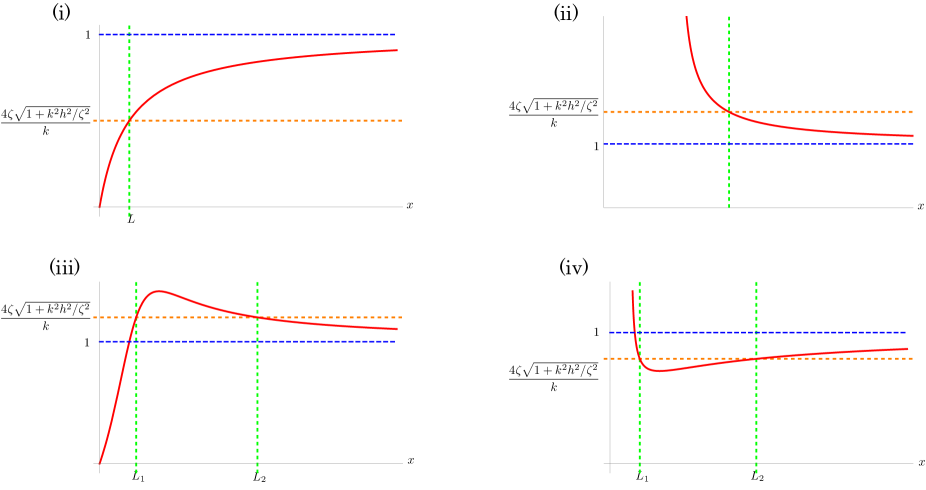
Figure 1: The behavior of the left-hand side of (C.12) for (i) $a\geq 0$ and $b\geq 0$, (ii) $a<0$ and $b\leq 0$, (iii) $a\geq 0$ and $b\leq 0$ and (iv) $a<0$ and $b\geq 0$.

For in the case (iii) and (iv), there exist two solutions $x=L_{1},L_{2}$ for (C.12) with $0\leq L_{1}<L_{2}$. Among them, the case (iii) ($a\geq 0,b\leq 0$) is excluded as $|{\widetilde{y}}_{o}|>1/4$ for $L_{1}<x<L_{2}$ which contradicts to our initial assumption. Hence the support $(L_{1},L_{2})$ could exist consistently only when the parameters satisfy $\zeta<k/4$, $h=0$, $a<0$ and $b>0$. On the other hand, in the case of (iv) we can easily find that there are no solutions $(a,b,L_{1},L_{2})$ ($0\leq L_{1}<L_{2}$) which also satisfy the first boundary condition in (C.8) $\rho\Delta_{e}(L_{1})=\rho\Delta_{e}(L_{2})=0$. Hence we conclude that the $x$-support $I_{x}$ cannot have any disconnected segment in the region $x>0$; it must always be in the form of $I_{x}=(-L,L)$.

In the case $I_{x}=(-L,L)$, in addition to the boundary constraint at $x=L$, we also require the smoothness of the profile functions at $x=0$. Indeed, any points where the profile functions are discontinuous require additional boundary constraints, with which the whole constraints become unsolvable as we have argued above. Then it is obvious that the case $h\neq 0$ is excluded. For the same reason we also find that $a$ and $b$ need to satisfy as $a>0$ and $b=0$. Under these restrictions the moduli $(a,b,B,L_{1})$ exist only when

$$\zeta<\frac{k}{4},$$ (C.13)

(see plot (i) in figure 1) and can be uniquely determined from the boundary constraint at $x=L$ and the normalization condition (C.7) as

$$a=\frac{k}{32\zeta^{2}}\Bigl{(}1-\frac{16\zeta^{2}}{k^{2}}\Bigr{)},\quad b=0,\quad B=\frac{\sqrt{k}}{4\sqrt{2}}\Bigl{(}1+\frac{16\zeta^{2}}{k^{2}}\Bigr{)},\quad I_{x}=\Bigl{(}-\frac{1}{\sqrt{2k}},\frac{1}{\sqrt{2k}}\Bigr{)}.$$ (C.14)

with which the explicit expression for the profile functions are

$${\widetilde{y}}_{e} =\sqrt{x^{2}+a},$$ (C.15)

$$\rho =4\zeta{\widetilde{y}}_{e}(1+{\widetilde{y}}_{e}^{\prime 2})=4\zeta\frac{d}{dx}(x{\widetilde{y}}_{e}),$$ (C.16)

$$\Delta_{e} =-\frac{1}{16m}\left(1-\frac{B{\widetilde{y}}_{e}}{\zeta({\widetilde{y}}_{e}^{2}+x^{2})}\right),$$ (C.17)

$$y_{o} =-\frac{1}{16m}\frac{Bx}{\zeta({\widetilde{y}}_{e}^{2}+x^{2})}.$$ (C.18)

The saddle point solution coincide with the solution I obtained in [10].

The free energy of this solution is

$$f=\frac{\pi\sqrt{2k}}{3}N^{\frac{3}{2}}\Bigl{(}1+\frac{16\zeta^{2}}{k^{2}}\Bigr{)},$$ (C.19)

as computed in [10].

We can check that the above solution of the saddle point equation corresponds to the solution we have introduced in section 3.2.2. To see this we express $x$ as a function of $s$ by integrating $\rho=ds/dx$

$$s(x)=\int_{0}^{x}dx\rho(x).$$ (C.20)

Using the explicit expression of $\rho$ (C.16) we obtain

$$x= \operatorname{sgn}(s)\sqrt{\frac{a}{2}}\sqrt{-1+\sqrt{1+\frac{4s^{2}(2a+1)}{a^{2}}}},$$ (C.21)

where

$$a=\frac{1}{2}\left(\frac{1}{16m^{2}}-1\right).$$ (C.22)

Hence ${\widetilde{y}}_{e}$ (C.15) is

$$\widetilde{y}_{e}= \sqrt{\frac{a}{2}}\sqrt{1+\sqrt{1+\frac{4s^{2}(2a+1)}{a^{2}}}}.$$ (C.23)

Now we can see that $x+iy_{e}$ coincides with $z_{1}(s)$ (3.61). Similarly, $\Delta_{e}+iy_{o}$ ((C.17) and (C.18)) expressed in terms of $s$ coincide with $z_{2}(s)$ (3.55).

References

- [1] K. Hosomichi, K. M. Lee, S. Lee, S. Lee and J. Park, “N=4 Superconformal Chern-Simons Theories with Hyper and Twisted Hyper Multiplets,” JHEP 0807 (2008) 091 doi:10.1088/1126-6708/2008/07/091 [arXiv:0805.3662 [hep-th]].
- [2] K. Hosomichi, K. M. Lee, S. Lee, S. Lee and J. Park, “N=5,6 Superconformal Chern-Simons Theories and M2-branes on Orbifolds,” JHEP 0809 (2008) 002 doi:10.1088/1126-6708/2008/09/002 [arXiv:0806.4977 [hep-th]].
- [3] J. Gomis, D. Rodriguez-Gomez, M. Van Raamsdonk and H. Verlinde, “A Massive Study of M2-brane Proposals,” JHEP 0809, 113 (2008) [arXiv:0807.1074 [hep-th]].
- [4] O. Aharony, O. Bergman, D. L. Jafferis and J. Maldacena, “N=6 superconformal Chern-Simons-matter theories, M2-branes and their gravity duals,” JHEP 0810, 091 (2008) [arXiv:0806.1218 [hep-th]].
- [5] S. Terashima, “On M5-branes in N=6 Membrane Action,” JHEP 0808, 080 (2008) [arXiv:0807.0197 [hep-th]].
- [6] Y. Kim, O. K. Kwon and D. D. Tolla, “Partially Supersymmetric ABJM Theory with Flux,” JHEP 1211 (2012) 169 doi:10.1007/JHEP11(2012)169 [arXiv:1209.5817 [hep-th]].
- [7] E. Witten, “Topological Quantum Field Theory,” Commun. Math. Phys. 117 (1988) 353. doi:10.1007/BF01223371
- [8] N. A. Nekrasov, “Seiberg-Witten prepotential from instanton counting,” Adv. Theor. Math. Phys. 7 (2003) 5, 831 doi:10.4310/ATMP.2003.v7.n5.a4 [hep-th/0206161].
- [9] V. Pestun, “Localization of gauge theory on a four-sphere and supersymmetric Wilson loops,” Commun. Math. Phys. 313 (2012) 71 doi:10.1007/s00220-012-1485-0 [arXiv:0712.2824 [hep-th]].
- [10] T. Nosaka, K. Shimizu and S. Terashima, “Large N behavior of mass deformed ABJM theory,” JHEP 1603 (2016) 063 doi:10.1007/JHEP03(2016)063 [arXiv:1512.00249 [hep-th]].
- [11] L. Anderson and K. Zarembo, “Quantum Phase Transitions in Mass-Deformed ABJM Matrix Model,” JHEP 1409, 021 (2014) doi:10.1007/JHEP09(2014)021 [arXiv:1406.3366 [hep-th]].
- [12] L. Anderson and J. G. Russo, “ABJM Theory with mass and FI deformations and Quantum Phase Transitions,” JHEP 1505, 064 (2015) [arXiv:1502.06828 [hep-th]].
- [13] T. Nosaka, K. Shimizu and S. Terashima, to appear.
- [14] J. G. Russo and K. Zarembo, “Evidence for Large-N Phase Transitions in N=2* Theory,” JHEP 1304 (2013) 065 doi:10.1007/JHEP04(2013)065 [arXiv:1302.6968 [hep-th]].
- [15] J. G. Russo and K. Zarembo, “Massive N=2 Gauge Theories at Large N,” JHEP 1311 (2013) 130 doi:10.1007/JHEP11(2013)130 [arXiv:1309.1004 [hep-th]].
- [16] Y. Imamura and K. Kimura, “On the moduli space of elliptic Maxwell-Chern-Simons theories,” Prog. Theor. Phys. 120 (2008) 509 doi:10.1143/PTP.120.509 [arXiv:0806.3727 [hep-th]].
- [17] S. Terashima and F. Yagi, “Orbifolding the Membrane Action,” JHEP 0812 (2008) 041 doi:10.1088/1126-6708/2008/12/041 [arXiv:0807.0368 [hep-th]].
- [18] O. Aharony, O. Bergman and D. L. Jafferis, “Fractional M2-branes,” JHEP 0811 (2008) 043 doi:10.1088/1126-6708/2008/11/043 [arXiv:0807.4924 [hep-th]].
- [19] N. Hama, K. Hosomichi and S. Lee, “Notes on SUSY Gauge Theories on Three-Sphere,” JHEP 1103 (2011) 127 doi:10.1007/JHEP03(2011)127 [arXiv:1012.3512 [hep-th]].
- [20] A. Kapustin, B. Willett and I. Yaakov, “Exact Results for Wilson Loops in Superconformal Chern-Simons Theories with Matter,” JHEP 1003 (2010) 089 doi:10.1007/JHEP03(2010)089 [arXiv:0909.4559 [hep-th]].
- [21] A. Kapustin, B. Willett and I. Yaakov, “Nonperturbative Tests of Three-Dimensional Dualities,” JHEP 1010 (2010) 013 doi:10.1007/JHEP10(2010)013 [arXiv:1003.5694 [hep-th]].
- [22] D. L. Jafferis, “The Exact Superconformal R-Symmetry Extremizes Z,” JHEP 1205 (2012) 159 doi:10.1007/JHEP05(2012)159 [arXiv:1012.3210 [hep-th]].
- [23] N. Drukker, J. Plefka and D. Young, “Wilson loops in 3-dimensional N=6 supersymmetric Chern-Simons Theory and their string theory duals,” JHEP 0811, 019 (2008) doi:10.1088/1126-6708/2008/11/019 [arXiv:0809.2787 [hep-th]].
- [24] B. Chen and J. B. Wu, “Supersymmetric Wilson Loops in N=6 Super Chern-Simons-matter theory,” Nucl. Phys. B 825 (2010) 38 [arXiv:0809.2863 [hep-th]].
- [25] S. J. Rey, T. Suyama and S. Yamaguchi, “Wilson Loops in Superconformal Chern-Simons Theory and Fundamental Strings in Anti-de Sitter Supergravity Dual,” JHEP 0903, 127 (2009) [arXiv:0809.3786 [hep-th]].
- [26] M. Marino, “Chern-Simons theory, matrix integrals, and perturbative three manifold invariants,” Commun. Math. Phys. 253 (2004) 25 doi:10.1007/s00220-004-1194-4 [hep-th/0207096].
- [27] M. Aganagic, A. Klemm, M. Marino and C. Vafa, “Matrix model as a mirror of Chern-Simons theory,” JHEP 0402 (2004) 010 doi:10.1088/1126-6708/2004/02/010 [hep-th/0211098].
- [28] N. Halmagyi and V. Yasnov, “The Spectral curve of the lens space matrix model,” JHEP 0911 (2009) 104 doi:10.1088/1126-6708/2009/11/104 [hep-th/0311117].
- [29] T. Suyama, “On Large N Solution of ABJM Theory,” Nucl. Phys. B 834 (2010) 50 doi:10.1016/j.nuclphysb.2010.03.011 [arXiv:0912.1084 [hep-th]].
- [30] D. L. Jafferis, I. R. Klebanov, S. S. Pufu and B. R. Safdi, “Towards the F-Theorem: N=2 Field Theories on the Three-Sphere,” JHEP 1106 (2011) 102 doi:10.1007/JHEP06(2011)102 [arXiv:1103.1181 [hep-th]].
- [31] I. R. Klebanov, S. S. Pufu and B. R. Safdi, “F-Theorem without Supersymmetry,” JHEP 1110 (2011) 038 doi:10.1007/JHEP10(2011)038 [arXiv:1105.4598 [hep-th]].
- [32] C. P. Herzog, I. R. Klebanov, S. S. Pufu and T. Tesileanu, “Multi-Matrix Models and Tri-Sasaki Einstein Spaces,” Phys. Rev. D 83, 046001 (2011) [arXiv:1011.5487 [hep-th]].
- [33] N. Drukker, M. Marino and P. Putrov, “From weak to strong coupling in ABJM theory,” Commun. Math. Phys. 306 (2011) 511 doi:10.1007/s00220-011-1253-6 [arXiv:1007.3837 [hep-th]].
- [34] S. Sugishita and S. Terashima, “Exact Results in Supersymmetric Field Theories on Manifolds with Boundaries,” JHEP 1311 (2013) 021 doi:10.1007/JHEP11(2013)021 [arXiv:1308.1973 [hep-th]].
- [35] D. Z. Freedman and S. S. Pufu, “The holography of -maximization,” JHEP 1403 (2014) 135 doi:10.1007/JHEP03(2014)135 [arXiv:1302.7310 [hep-th]].