Node Overlap Removal by Growing a Tree

Abstract

Node overlap removal is a necessary step in many scenarios including laying out a graph, or visualizing a tag cloud. Our contribution is a new overlap removal algorithm that iteratively builds a Minimum Spanning Tree on a Delaunay triangulation of the node centers and removes the node overlaps by ”growing” the tree. The algorithm is simple to implement yet produces high quality layouts. According to our experiments it runs several times faster than the current state-of-the-art methods.

1 Introduction

Removing node overlap after laying out a graph is a common task in network visualization. Most graph layout algorithms [23] consider nodes as points that do not occupy any geometrical space. In practice, nodes often have shapes, labels, and so on. These shapes and labels may overlap in the visualization and affect the visual readability. To remove such overlaps a specialized algorithm is usually applied.

The main contribution of this paper is a new node overlap removal algorithm that we call Growing Tree, or GTree further on. The basic idea is to first capture most of the overlap and the local structure with a specific spanning tree on top of a proximity graph, and then resolve the overlap by letting the tree ”grow”.

We compare GTree with PRISM [6], which is widely used for the same purpose. Needing more area than PRISM, our method preserves the original layout well and is up to eight times faster than PRISM. To compare the two algorithms we implemented GTree in the open source graph visualization software Graphviz , where PRISM is the default overlap removal algorithm. On the other side, GTree is the default in MSAGL, where we also have an implementation of PRISM. We ran comparisons by using both tools.

2 Related Work

There is vast research on node overlap removal. Some methods, including hierarchical layouts [4], incorporate the overlap removal with the layout step. Likewise, force-directed methods [5] have been extended to take the node sizes into account [17, 16, 24], but it is difficult to guarantee overlap-free layouts without increasing the repulsive forces extensively. Dwyer et al. [2] show how to avoid node overlaps with Stress Majorization [7]. The method can remove node overlaps during the layout step, but it needs an initial state that is overlap free; sometimes such a state is not given.

Another approach, which we also choose, is to use a post-processing step. In Cluster Busting [18, 8] the nodes are iteratively moved towards the centers of their Voronoi cells. The process has the disadvantage of distributing the nodes uniformly in a given bounding box.

Imamichi et al. [15] approximate the node shapes by circles and minimize a function penalizing the circle overlaps.

Starting from the center of a node, RWorldle [22] removes the overlaps by discovering the free space around a node by using a spiral curve and then utilizing this space. The approach requires a large number of intersection queries that are time consuming. This idea is extended by Strobelt et al. [21] to discover available space by scanning the plane with a line or a circle.

Another set of node overlap removal algorithms focus on the idea of defining pairwise node constraints and translating the nodes to satisfy the constraints [20, 11, 19, 13]. These methods consider horizontal and vertical problems separately, which often leads to a distorted aspect ratio [6]. A Force-transfer-algorithm is introduced by Huang et al. [14]; horizontal and vertical scans of overlapped nodes create forces moving nodes vertically and horizontally; the algorithm takes $\mathcal{O}(n^{2})$ steps, where $n$ is the number of the nodes. Gomez et al. [9] develop Mixed Integer Optimization for Layout Arrangement to remove overlaps in a set of rectangles. The paper discusses the quality of the layout, which seems to be high, but not the effectiveness of the method, which relies on a mixed integer problem solver. Dwyer et al. [3] reduce the overlap removal to a quadratic problem and solve it efficiently in $\mathcal{O}(n\log n)$ steps. According to Gansner and Hu [6], the quality and the speed of the method of Dwyer et al. [3] is very similar to the ones of PRISM.

The ProjSnippet method [10] generates good quality layouts. The method requires $\mathcal{O}(n^{2})$ amount of memory, at least if applied directly as described in the paper, and the usage of a nonlinear problem solver.

In PRISM [6, 12], a Delaunay triangulation on the node centers is used as the starting point of an iterative step. Then a stress model for node overlap removal is built on the edges of the triangulation and the stress function of the model is minimized. GTree also starts with building this Delaunay triangulation, but then the algorithms diverge.

3 GTree Algorithm

An input to GTree is a set of nodes $V$, where each node $i\in V$ is represented by an axis-aligned rectangle $B_{i}$ with the center $p_{i}$. We assume that for different $i,j\in V$ the centers $p_{i},p_{j}$ are different too. If this is not the case, we randomly shift the nodes by tiny offsets. We denote by $D$ a Delaunay triangulation of the set $\{p_{i}:i\in V\}$, and let $E$ be the set of edges of $D$.

On a high level, our method proceeds as follows. First we calculate the triangulation $D$, then we define a cost function on $E$ and build a minimum cost spanning tree on $D$ for this cost function. Finally, we let the tree “grow”. The steps are repeated until there are no more overlaps. The last several steps are slightly modified. Now we explain the algorithm in more detail.

We define the cost function $c$ on $E$ in such a way that the larger the overlap on an edge becomes, the smaller the cost of this edge comes to be. Let $(i,j)\in E$. If the rectangles $B_{i}$ and $B_{j}$ do not overlap then $c(i,j)=dist(B_{i},B_{j})$, that is the distance between $B_{i}$ and $B_{j}$. Otherwise, for a real number $t$ let us denote by $B_{j}(t)$ a rectangle with the same dimensions as $B_{j}$ and with the same orientation, but with the center at $p_{i}+t(p_{j}-p_{i})$. We find $t_{ij}>1$ such that the rectangles $B_{i}$ and $B_{j}(t_{ij})$ touch each other. Let $s=\|p_{j}-p_{i}\|$, where $\|\|$ denotes the Euclidean norm. We set $c(i,j)=-(t_{ij}-1)s$. See Figure 1 for an illustration.

Figure 1: Cost function $c_{ij}$ for edges of the Delaunay triangulation. For overlapping nodes $-c_{ij}$ is equal to the minimal distance that is necessary to shift the boxes along the edge direction so they touch each other.

Having the cost function ready, we compute a minimum spanning tree $T$ on $D$. Remember that it is a tree with the set of vertices $V$ for which the cost, $\sum_{e\in E^{\prime}}{c(e)}$, is minimal, where $E^{\prime}$ is the set of edges of the tree. We use Prim’s algorithm to find $T$.

The algorithm proceeds by growing $T$, similar to the growth of a tree in nature. It starts from the root of $T$. For each child of the root overlapping with the root, it extends the edge connecting the root and the child to remove the overlap. To achieve this, it keeps the root fixed but translates the sub-tree of the child. The edges between the root and other children remain unchanged. The algorithm recursively processes the children of the root in the same manner. This process is described in Algorithm 1.

1

Input: Current center positions $p$ and root $r$

Output: New center positions $p^{\prime}$

2 $p^{\prime}_{r}=p_{r}$

3 GrowAtNode $(r)$

4

5function GrowAtNode (i)

6       foreach $j\in\text{Children}(i)$ do

7             $p^{\prime}_{j}=p^{\prime}_{i}+t_{ij}(p_{j}-p_{i})$

8             GrowAtNode (j);

9      

Algorithm 1 Growing $T$

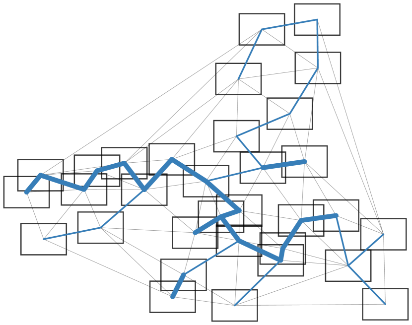
(a) iteration 1

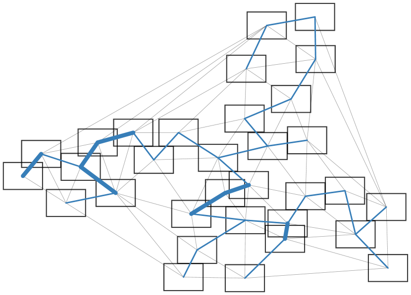
(b) iteration 2

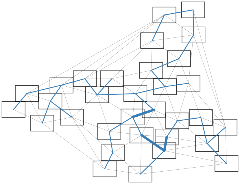
(c) iteration 3

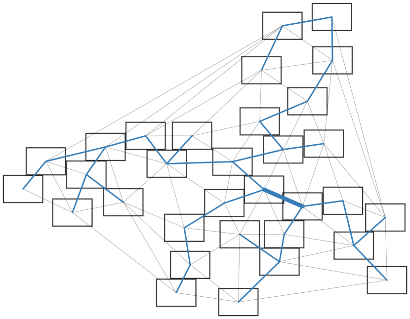
(d) iteration 4

(e) iteration 5

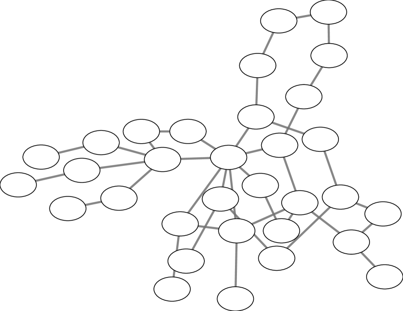
(f) final overlap free graph
with original shapes

Figure 2: Overlap removal process with the minimum spanning tree on the proximity graph, where the latter here is a Delaunay triangulation on rectangle centers. The blue edges form a tree; there are four different trees in the figure. The tree edges connecting overlapped nodes are thick and solid. In each iteration the thick edges are elongated and the dashed tree edges shift accordingly. Overlap is completely resolved in four iterations.

The number $t_{ij}$ in line 1 of Algorithm 1 is the same as in the definition of the cost of the edge $(i,j)$ when $B_{i}$ and $B_{j}$ overlap, and is $1$ otherwise.

The algorithm does not update all positions for the child sub-tree nodes immediately, but updates only the root of the sub-tree. Using the initial positions of a parent and a child, and the new position of the parent, the algorithm obtains the new position of the child in line 1. In total, Algorithm 1 works in $O(|V|)$ steps. The choice of the root of the tree does not matter. Different roots produce the same results modulo a translation of the plane by a vector. Indeed it can be shown that after applying the algorithm, for any $i,j\in V$ the vector $p^{\prime}_{j}-p^{\prime}_{i}$ is defined uniquely by the path from $i$ to $j$ in $T$.

While an overlap along any edge of the triangulation exists, we iterate, starting from finding a Delaunay triangulation, then building a minimum spanning tree on it, and finally running Algorithm 1. See Figure 2 for an example.

When there are no overlaps on the edges of the triangulation, as noticed by Gansner and Hu [6], overlaps are still possible. We follow the same idea as PRISM and modify the iteration step. In addition to calculating the Delaunay triangulation we run a sweep-line algorithm to find all overlapping node pairs and augment the Delaunay graph $D$ with each such a pair. As a consequence, the resulting minimum spanning tree contains non-Delaunay edges catching the overlaps, and the rest of the overlaps are removed. This stage usually requires much less time than the previous one.

It is possible to create an example where the algorithm will not remove all overlaps. However, such examples are extremely rare and have not been seen yet in practice of using MSAGL or in our experiments. MSAGL applies random tiny changes to the initial layout which prevents GTree from cycling.

4 Comparing PRISM and GTree by Measuring Layout Similarity, Quality, and Run Time

Our data includes the same set of graphs that was used by the authors of PRISM to compare it with other algorithms [6]. The set is available in the Graphviz open source package. We also used a small collection of random graphs and a collection of about 10,000 files. For the experiments we use a modified version of Dot, where we can invoke either GTree or Prism for the overlap removal step, and we also used MSAGL, where we implemented PRISM and GTree. MSAGL was used only to obtain the quality measures. We ran the experiments on a PC with Linux, 64bit and an Intel Core i7-2600K CPU@3.40GHz with 16GB RAM.

Some of resulting layouts can be seen in Figures 3,  5,  6.

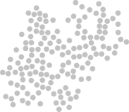
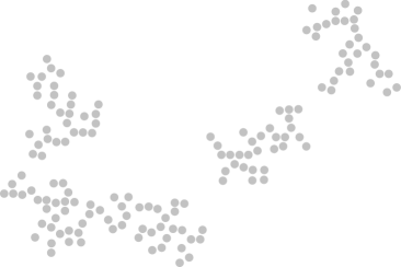
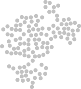
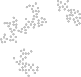
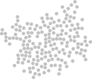
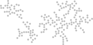
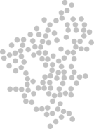
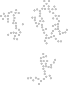
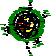
PRISM	original layout	GTree

Figure 3: Comparison between PRISM, original, and GTree layouts. In four top rows the initial layouts were generated randomly. At the bottom are the drawings of nodes of graph ”root” which was initially laid out by the Multi Dimensional Scaling algorithm of MSAGL. In our opinion, the initial structure is more preserved in the right column, containing the results of GTree.

One can try to resolve overlap by scaling the node centers of the original layout. If there are no two coincident node centers this will work, but the resulting layout may require a huge area if some centers are close to each other. We consider the area of the final layout as one of the quality measures, and usually PRISM produces a smaller area than GTree, see Table 1.

In addition to comparing the areas, we compare some other layout properties. Following Gansner and Hu [6], we look at edge length dissimilarity, denoted as $\sigma_{\text{edge}}$. This measure reflects the relative change of the edge lengths of a Delaunay Triangulation on the node centers of the original layout.

The other measure, which is denoted by $\sigma_{disp}$, is the Procrustean similarity [1]. It shows how close the transformation of the original graph is to a combination of a scale, a rotation, and a shift transformation. PRISM and GTree performs similar in the last two measures as Table 1 shows.

To distinguish the methods further, we measure the change in the set of $k$ closest neighbors of the nodes. Namely, let $p_{1},\dots,p_{n}$ be the positions of the node centers, and let $k$ be an integer such that $0<k\leq n$. Let $I=\{1,\dots,n\}$ be the set of node indices. For each $i\in I$ we define $N_{k}(i)\subset I\setminus\{i\}$, such that $|N_{k}(p,i)|=k$, and for every $j\in I\setminus N_{k}(p,i)$ and for every $j^{\prime}\in N_{k}(p,i)$ holds $\|p_{j}-p_{i}\|\geq\|p_{j^{\prime}}-p_{i}\|$. In other words, $N_{k}(p,i)$ represents a set of $k$ closest neighbors of $i$, excluding $i$. Let $p^{\prime}_{1},\dots,p^{\prime}_{n}$ be transformed node centers. To see how much the layout is distorted nearby node $i$, we intersect $N_{k}(p,i)$ and $N_{k}(p^{\prime},i)$. We measure the distortion as $(k-m)^{2}$, where $m$ is the number of elements in the intersection. One can see that if the node preserves its $k$ closest neighbors then the distortion is zero.

Our experiments for $k$ from $8$ to $12$ show that under this measure GTree produced a smaller error, showing less distortion, on 8 graphs from 14, and on the rest PRISM produced a better result, see Table 2. GTree produced a smaller error on all small random graphs from other collections.

Table 1: Similarity to the initial layout (left) and number of iterations for different graph sizes and different initialization methods (right). PR stands for PRISM

	$\sigma_{\text{edge}}$		$\sigma_{\text{disp}}$		area
Graph	PR	GTree	PR	GTree	PR	GTree
dpd	0.34	0.28	0.37	0.36	0.82	0.84
unix	0.22	0.19	0.24	0.20	2.38	2.38
rowe	0.29	0.26	0.23	0.24	0.68	0.73
size	0.39	0.37	0.24	0.26	1.09	1.28
ngk10_4	0.30	0.30	0.27	0.30	0.00	0.00
NaN	0.56	0.44	0.73	0.51	4.03	4.34
b124	0.55	0.53	0.97	0.83	5.52	6.22
b143	0.67	0.70	1.12	0.93	3.62	3.88
mode	0.54	0.50	0.59	0.53	1.53	2.29
b102	0.71	0.77	1.43	1.27	4.50	6.62
xx	0.75	0.70	1.65	1.42	6.21	9.57
root	1.09	1.19	2.89	2.45	34.58	91.87
badvoro	0.88	0.92	2.27	2.42	25.68	47.43
b100	0.84	0.98	3.08	3.14	20.64	37.38

init. layout:		neato			SFDP
Graph	$|V|$	$|E|$	PR	GTree	PR	GTree
dpd	36	108	4	7	3	6
unix	41	49	3	4	12	5
rowe	43	68	5	4	13	7
size	47	55	7	3	9	5
ngk10_4	50	100	6	3	14	7
NaN	76	121	8	3	24	6
b124	79	281	14	4	30	12
b143	135	366	21	6	37	12
mode	213	269	37	8	11	6
b102	302	611	60	24	113	19
xx	302	611	83	18	50	19
root	1054	1083	95	18	99	22
badvoro	1235	1616	40	20	50	23
b100	1463	5806	80	24	136	28

Table 2: k closest neighbors error, the Multi Dimensional Scaling algorithm of MSAGL was used for the initial layout. PR stands for PRISM.

	$k=8$		$k=9$		$k=10$		$k=11$		$k=12$
Graph	PR	GTree	PR	GTree	PR	GTree	PR	GTree	PR	GTree
dpd	7.75	6.06	9.61	7.36	9.5	8	10.14	8.5	9.97	7.64
unix	8.56	7.05	10.51	8.8	10.95	10.02	11.66	10.54	13	11.41
rowe	6.28	8.09	7.09	9.95	7.49	10.49	9.12	11.4	11.05	12.51
size	4.68	6.09	5.47	6.47	6.28	7.57	6.89	8.13	8.26	10.02
ngk10_4	6.76	7.4	7.52	9.26	8.28	11.38	10.72	13.74	11.92	14.66
NaN	11.83	8.95	14.46	11.5	17.32	13.88	19.88	16.37	22.17	19.7
b124	11.03	11.44	13.22	13.56	14.76	15.54	15.91	17.32	18.23	20.04
b143	13.49	12.39	16.31	14.99	19.49	17.93	23.11	21.04	26.53	24.43
mode	16.91	11.46	20.58	13.95	24.68	16.85	29.54	19.92	34.48	22.56
b102	15.99	14.62	19.61	18.78	23.38	22.77	27.28	26.77	32.15	31.45
xx	15.68	15.65	19.01	19.45	23.05	23.37	26.98	27.35	31.29	32.47
root	17.09	15.7	20.89	19.36	25.48	23.3	30.48	27.66	35.74	32.83
badvoro	16.18	15.15	20.16	18.98	24.37	23.28	29.18	28.03	34.29	33.29
b100	18	19.25	22.11	23.65	26.79	28.69	32.03	34.46	37.44	40.5

We ran tests on the graphs from a subdirectory of the same site called “dot_files”, let us call this set of graphs collection $A$. Each graph from $A$ represents the control flow of a method from a version of the .NET framework. $A$ contains 10077 graphs. The graph sizes do not exceed several thousands. We used the Multi Dimensional Scaling algorithms of MSAGL for the initial layout in this test. The results of the run are summarized in Table 3.

Table 3: Statistics on collection $A$. Here k-cn stands for k-closest neighbors, and “iters” stands for the number of iterations. Each cell contains the number of graphs for the measure on which the method performed better. We can see that PRISM produced a layout of smaller area than the one of GTree on 8498 graph, against 1579 graphs where GTree required less area. From the other side, GTree gives better results on all other measures. The columns of k-cn and “iters” do not sum to 10077, the number of graphs in $A$, because some of the results were equal for PRISM and GTree.

Method	k-cn	$\sigma_{\text{edge}}$	$\sigma_{\text{disp}}$	area	iters	time
PRISM	3237	4741	4114	8498	46	7
GTree	4088	5336	5963	1579	9986	10070

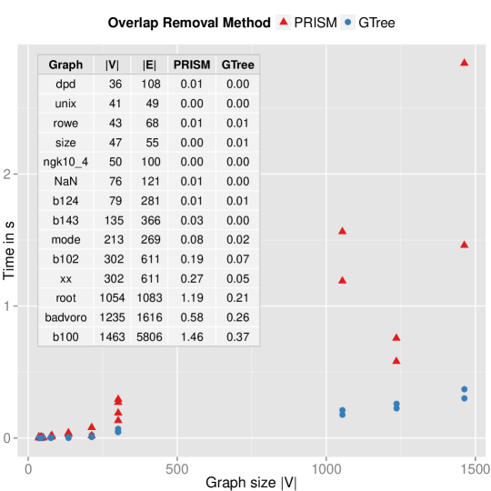
Figure 4: Runtimes for PRISM and GTree.

Runtime Comparison

Both methods remove the overlap iteratively using the proximity graph. However, while PRISM needs $\mathcal{O}(|V|\cdot\sqrt{|V|})$ time to solve the stress model, GTree needs only $\mathcal{O}(|V|)$ time per iteration with the growing tree procedure. Therefore, GTree is asymptotically faster in a single iteration. In addition, as Table 1 (right) shows, GTree usually needs fewer iterations than PRISM, especially on larger graphs. The overall runtime can be seen in Figure 4. It shows that GTree outperforms PRISM on larger graphs.

(a) initial layout

(b) PRISM

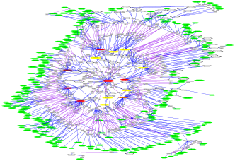
(c) GTree

Figure 5: root graph with 1054 nodes and 1083 edges. (a) initial layout with NEATO, (b) applying PRISM, (c) applying GTree.

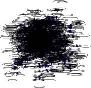
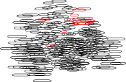
GTree	original	PRISM

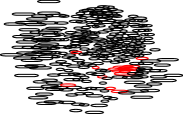
GTree	original	PRISM

Figure 6: Results for GTree and PRISM initialized with SFDP. From top to bottom and left to right: b100, b102, b124, b143, badvoro, dpd, mode, - NaN, ngk10_4, root, rowe, size, unix, and xx. To make the original drawings more readable they have been changed; In most cases the nodes were diminished and the edges removed. The drawings were scaled differently.

In Figure 5 we experiment with the way we expand the edges. Instead of the formula $p^{\prime}_{j}=p^{\prime}_{i}+t_{ij}(p_{j}-p_{i})$, which resolves the overlap between the nodes $i$ and $j$ immediately, we use the update $p^{\prime}_{j}=p^{\prime}_{i}+\min(t_{ij},1.5)(p_{j}-p_{i})$. As a result, the algorithm runs a little bit slower but produces layouts with smaller area.

5 Conclusion & Future Work

We proposed a new overlap removal algorithm that uses the minimum spanning tree. The algorithm is simple and easy to implement, and yet it preserves the initial layout well and is efficient.

Although we introduced our approach in the context of graph visualization, our method can also be used for any other purpose where overlap needs to be resolved while maintaining the initial layout. Finding a measure of how well an overlap removal algorithm preserves clusters of the initial layout seems to be an interesting challenge.

References

- [1] I. Borg and P. Groenen. Modern multidimensional scaling: Theory and applications. Springer, 2005.
- [2] T. Dwyer, Y. Koren, and K. Marriott. Ipsep-cola: An incremental procedure for separation constraint layout of graphs. IEEE Trans. Vis. Comput. Graph., 12(5):821–828, 2006.
- [3] T. Dwyer, K. Marriott, and P. J. Stuckey. Fast node overlap removal. In Graph Drawing, pages 153–164. Springer, 2006.
- [4] C. Friedrich and F. Schreiber. Flexible layering in hierarchical drawings with nodes of arbitrary size. In V. Estivill-Castro, editor, ACSC, volume 26 of CRPIT, pages 369–376. Australian Computer Society, 2004.
- [5] T. M. J. Fruchterman and E. M. Reingold. Graph drawing by force-directed placement. Software - Practice and Experience, 21(11):1129–1164, 1991.
- [6] E. R. Gansner and Y. Hu. Efficient, proximity-preserving node overlap removal. J. Graph Algorithms Appl., 14(1):53–74, 2010.
- [7] E. R. Gansner, Y. Koren, and S. C. North. Graph drawing by stress majorization. In J. Pach, editor, Graph Drawing, volume 3383 of Lecture Notes in Computer Science, pages 239–250. Springer, 2004.
- [8] E. R. Gansner and S. C. North. Improved force-directed layouts. In S. Whitesides, editor, Graph Drawing, volume 1547 of Lecture Notes in Computer Science, pages 364–373. Springer, 1998.
- [9] E. Gomez-Nieto, W. Casaca, L. G. Nonato, and G. Taubin. Mixed integer optimization for layout arrangement. In Graphics, Patterns and Images (SIBGRAPI), 2013 26th SIBGRAPI-Conference on, pages 115–122. IEEE, 2013.
- [10] E. Gomez-Nieto, F. San Roman, P. Pagliosa, W. Casaca, E. Helou, M. Ferreira de Oliveira, and L. Nonato. Similarity preserving snippet-based visualization of web search results. 2013.
- [11] K. Hayashi, M. Inoue, T. Masuzawa, and H. Fujiwara. A layout adjustment problem for disjoint rectangles preserving orthogonal order. Systems and Computers in Japan, 33(2):31–42, 2002.
- [12] Y. Hu. Visualizing graphs with node and edge labels. CoRR, abs/0911.0626, 2009.
- [13] X. Huang and W. Lai. Force-transfer: A new approach to removing overlapping nodes in graph layout. In M. J. Oudshoorn, editor, ACSC, volume 16 of CRPIT, pages 349–358. Australian Computer Society, 2003.
- [14] X. Huang, W. Lai, A. Sajeev, and J. Gao. A new algorithm for removing node overlapping in graph visualization. Information Sciences, 177(14):2821–2844, 2007.
- [15] T. Imamichi, Y. Arahori, J. Gim, S.-H. Hong, and H. Nagamochi. Removing node overlaps using multi-sphere scheme. In I. G. Tollis and M. Patrignani, editors, Graph Drawing, volume 5417 of Lecture Notes in Computer Science, pages 296–301. Springer, 2008.
- [16] W. Li, P. Eades, and N. S. Nikolov. Using spring algorithms to remove node overlapping. In S.-H. Hong, editor, APVIS, volume 45 of CRPIT, pages 131–140. Australian Computer Society, 2005.
- [17] C.-C. Lin, H.-C. Yen, and J.-H. Chuang. Drawing graphs with nonuniform nodes using potential fields. J. Vis. Lang. Comput., 20(6):385–402, 2009.
- [18] K. A. Lyons, H. Meijer, and D. Rappaport. Algorithms for cluster busting in anchored graph drawing. J. Graph Algorithms Appl., 2(1), 1998.
- [19] K. Marriott, P. J. Stuckey, V. Tam, and W. He. Removing node overlapping in graph layout using constrained optimization. Constraints, 8(2):143–171, 2003.
- [20] K. Misue, P. Eades, W. Lai, and K. Sugiyama. Layout adjustment and the mental map. J. Vis. Lang. Comput., 6(2):183–210, 1995.
- [21] H. Strobelt, M. Spicker, A. Stoffel, D. Keim, and O. Deussen. Rolled-out wordles: A heuristic method for overlap removal of 2d data representatives. In Computer Graphics Forum, volume 31, pages 1135–1144. Wiley Online Library, 2012.
- [22] H. Strobelt, M. Spicker, A. Stoffel, D. A. Keim, and O. Deussen. Rolled-out wordles: A heuristic method for overlap removal of 2d data representatives. Comput. Graph. Forum, 31(3):1135–1144, 2012.
- [23] R. Tamassia. Handbook of Graph Drawing and Visualization (Discrete Mathematics and Its Applications). Chapman & Hall/CRC, 2007.
- [24] X. Wang and I. Miyamoto. Generating customized layouts. In F.-J. Brandenburg, editor, Graph Drawing, volume 1027 of Lecture Notes in Computer Science, pages 504–515. Springer, 1995.