Allocation of risk capital in a cost cooperative game induced by a modified Expected Shortfall

Abstract

The standard theory of coherent risk measures fails to consider individual institutions as part of a system which might itself experience instability and spread new sources of risk to the market participants. In compliance with an approach adopted by Shapley and Shubik (1969), this paper proposes a cooperative market game where agents and institutions play the same role can be developed. We take into account a multiple institutions framework where some of them jointly experience distress events in order to evaluate their individual and collective impact on the remaining institutions in the market. To carry out this analysis, we define a new risk measure ($SCoES$), generalising the Expected Shortfall of Acerbi (2002) and we characterise the riskiness profile as the outcome of a cost cooperative game played by institutions in distress (a similar approach was adopted by Denault 2001). Each institution’s marginal contribution to the spread of riskiness towards the safe institutions in then evaluated by calculating suitable solution concepts of the game such as the Banzhaf–Coleman and the Shapley–Shubik values.

Keywords: Cooperative market game, Shapley Value, risk measures, Value–at–Risk, expected shortfall, systemic risk.

1 Introduction

The assessment of financial risk in a multi–institution framework when some institutions are subject to systemic or non–systemic distress is one of the main topics of the latest years which received large attention from scholars in Mathematical Finance, Statistics, Management, see, e.g., Adrian and Brunnermeier (2011, 2016), Billio et al. (2012), Acharya et al. (2012), Girardi and Ergün (2013), Hautsch et al. (2014), Engle et al. (2014), Lucas et al. (2014), Bernardi and Catania (2015), Sordo et al. (2015), just to quote a few of the most relevant approaches. For an extensive and up to date survey on systemic risk measures, see Bisias et al. (2012), while the recent literature on systemic risk is reviewed by Benoit et al. (2016). Especially since 2008, Lehmann Brothers’ collapse and the subsequent debt crisis contagion across Europe raised crucial issues and questions to be addressed by new macroeconomic and financial models. In particular, such events and the related consequences provoked a wide increase in investigation of instruments possibly suitable for risk evaluation, thereby targeting the occurrence of contagion among institutions in distress (see, among others, Drehmann and Tarashev 2013 on the theoretical side and Huang et al. 2012a and Huang et al. 2012b on the empirical side).
In this paper we are going to investigate circumstances where one or more market institutions undergo financial distress and may spread the contagion to the remaining safe institutions in the market. Financial distress has a straightforward meaning: a condition of dramatic financial instability of an institution, or lack of ability to fully repay its creditors, or even the preliminary to bankruptcy or liquidation. Although “financial distress” and “default” are sometimes used interchangeably, there may be some differences, often depending either on each country’s specific bankruptcy law or on the institution’s rating and so on (see Altman and Hotchkiss 2010 for an extensive discussion).
When a financial distress takes place in the market, each distressed institution affects the safe ones and individually contributes to the systemic risk. A crucial aspect of the contagion frameworks is the assessment of each agent’s (i.e. each institution’s) marginal effect on systemic risk. In order to evaluate such contributions, a natural and intuitive tool is the Shapley value (see Shapley 1988), as well as the Banzhaf value (see Banzhaf III 1965 and Owen 1995). It is interesting to note that, although his world famous theories did not concern financial markets specifically, L.S. Shapley, Nobel Laureate in Economic Sciences in 2012, proposed a relevant application to market analysis in a paper with M. Shubik in 1969 (see Shapley and Shubik 1969). In that paper, Shapley and Shubik defined and investigated the direct markets (see Shapley and Shubik (1969), pp. 15–18), i.e., markets where, since each trader possessed one initial unit of a personal commodity, traders might be identified with commodities. As the Authors put it literally, “A canonical market form – the direct market – is introduced, in which the commodities are in effect the traders themselves, made infinitely divisible…” (p. 11), hence that was the first attempt to model a cooperative game where agents had a twice nature: traders and assets at the same time.
Hence, classical solution concepts widely used in Cooperative Game Theory such as the Shapley value and the Banzhaf value fit our evaluation purposes. In more recent times, cooperative game theory has already been employed for risk capital allocation by Denault (2001) and in the latest years by Csóka et al. (2009) and Abbasi and Hosseinifard (2013). However, in none of the above papers a characteristic value expressing the difference between an expected value in a non–distressed case and an expected value in a distressed–case has been taken into account.
The financial setup we are going to investigate involves a set of possibly distressed institutions (for example a set of banks) and a set of safe institutions. Our purpose is an assessment of the contagion risk, i.e., the extent to which the safe institutions can be affected and damaged by the financial distress of the unsafe ones. For this purpose, risk measures have been extensively theorized and analyzed, giving rise to a rich strand of literature. Some of them might provide helpful techniques for risk allocation among a number of distinct systemic agents. In this respect, the coherent risk measures have been and are a crucial tool for the assignment of risk capital, both for the richness of properties due to their axiomatic structure and for their adaptability to fit several financial frameworks. The basic studies on coherent risk measures have been published by Artzner et al. (1999) in 1999, who first provided an axiomatic characterization. Subsequently, in 2001 Denault (2001) developed the analysis by taking into account a cooperative game structure, where players are the firms involved in risky financial activities, and the risk induced by the net worth of firms is the value of the characteristic function of the game, and the subadditivity axiom naturally induces a cost cooperative game.
The coherence of the Expected Shortfall (ES, hereafter) was taken into account by Acerbi and Tasche (2002) in 2002, whereas an axiomatic approach was adopted in 2005 by Kalkbrener (2005), to characterize the related capital allocation procedures in portfolio management or performance measurement. In recent years, further mathematical results were achieved by Stoica (2006) (equivalence between properties of some coherent measures with no arbitrage conditions), Csóka et al. (2007, 2009) (refinement of measures in a general equilibrium setup, stability of risk allocations), Kountzakis and Polyrakis (2013) (applications to general equilibrium models). Other relevant results in risk allocation theory were provided in Drehmann and Tarashev (2013) and Csóka and Pintér (2016). Furthermore, as a slightly different tool, distortion risk measures have been applied to a financial contagion framework by Cherubini and Mulinacci (2014).
The new approach we are going to propose builds on an alternative risk measure which is an extension of ES and which is supposed to incorporate the effect of the distressed institutions on a safe one. Such a measure, denoted by $SCoES_{i|\mathcal{D}}^{\tau_{1}|\tau_{2}}$, represents the expected value of a non–distressed institution $i$ conditional upon a set $\mathcal{D}$ of institutions under distress, given two different thresholds $\tau_{1},\tau_{2}\in\left(0,1\right)$, specifically related to the institutions’ returns. Subsequently, in order to evaluate the marginal contribution of each distressed institution to overall systemic risk, we will construct a cost function. Such a function aims to measure the cost of risk by evaluating the mean of the differences between the standard Expected Shortfalls and the values of $SCoES$ of all non–distressed institutions. This formula will be the characteristic value of a cooperative game played by distressed institutions. Adopting a classical approach, we will examine the properties of the game and calculate the marginal impacts of each distressed institution, pointing out the differences between the Shapley value and the Banzhaf value of the game.
The introduced risk measurement framework is then adopted to empirically analyze the evolution of the $SCoES$ risk measure and the output of the associated cooperative game of risk for eight Eurozone sovereign Credit Default Swaps (CDS) over the period 2008–2014. Our example assumes the Germany as the “safe” country, and explores how the evolution of the remaining countries’ debt conditions affect the health and financial stability of Germany considered as a “proxy” for the overall European system. As a byproduct of the proposed risk framework, the evolution of the total impact of the failure of the European system is monitored. Our results show that the risk of failure of the European system displays a transitory high level during period in between the Greece and Portugal bailouts (November 2010 – May 2011), but effectively remains at high levels when the ECB president Mario Draghi announces the implementation of the Outright Monetary Transactions (OMT) and the European Stability Mechanism (ESM) in the months thereafter. It is only after the implementation of the OMT, and the ESM, that the systemic risk of Germany settles more permanently at a level that is roughly 60% lower than during the crisis.
The remainder of the paper is structured as follows. In Section 2 the basic concepts about risk measures will be recalled, together with some axiomatic details of coherent measures. Section 3 introduces the indicators that will be crucial to our analysis, whereas in Section 4 the cooperative game of risk and its solution concepts are exposed and discussed. Section 5 is devoted to the empirical application and Section 6, conclusions and possible future developments are laid out.

2 Risk measures in portfolio management

Here we will outline the standard notation for risk measurement in recent literature, largely borrowed from the seminal paper by Artzner Artzner et al. (1999) and Kalkbrener (2005).

Consider a finite set of states of nature $\Omega$, whose cardinality is $|\Omega|=m$. Call $X(\omega_{j})$ a random variable indicating the final net worth of a position in state $\omega_{j}\in\Omega$ after a certain time interval, i.e., the possible profit and loss realization of a portfolio in state $\omega_{j}$. We can identify the set of all real-valued functions (which can also be viewed as the set of all risks) on $\Omega$ as $\mathbb{R}^{m}$, whose elements are of the kind $X=(X(\omega_{1}),\ldots,X(\omega_{m}))$. In the rigorous construction proposed in Artzner et al. (1999), a measure of risk is a mapping $\rho:\mathbb{R}^{m}\longrightarrow\mathbb{R}$ such that $\rho(X)$ corresponds to the minimum amount of extra cash an agent has to add to her risky portfolio, in order to ensure that this investment is still acceptable to the regulator when using a suitable reference instrument. The basic requirement concerns the price of the asset: 1 is the initial price of the asset and $r>0$ is the total return on the reference instrument at a final date $T$, in all possible states of nature. In Artzner et al. (1999) the Definition of a coherent measure is then provided based on an axiomatic structure.

Definition 1.

A function $\rho:\mathbb{R}^{S}\longrightarrow\mathbb{R}$ is called a coherent measure of risk if it satisfies the following axioms:

• Monotonicity (M): for all $X,Y\in\mathbb{R}^{m}$ such that $Y\geq X$ (i.e. $Y(\omega_{j})\geq X(\omega_{j})$ for almost all $\omega_{j}\in\Omega$), $\rho(Y)\leq\rho(X)$.

• Subadditivity (S): for all $X,Y\in\mathbb{R}^{m}$, $\rho(X+Y)\leq\rho(X)+\rho(Y)$.

• Positive Homogeneity (PH): for all $X\in\mathbb{R}^{m}$ and $\lambda\in\mathbb{R}_{+}$, $\rho(\lambda X)=\lambda\rho(X)$.

• Translation Invariance (TI): for all $X\in\mathbb{R}^{m}$ and $h\in\mathbb{R}$,

  $$\rho(X+hr)=\rho(X)-h.$$

We have to point out that the Value-at-Risk ($VaR$) satisfies all of them except Subadditivity, as is precisely exposed in Artzner et al. (1999) as well as the standard Definition of $VaR$, which is recalled here:

Definition 2.

Given $\tau\in[0,1]$ and the return on a reference instrument $r>0$, the $VaR$ at level $\tau$ of the final net worth $X$ with probability $\mathbb{P}\left\{\cdot\right\}$ is the negative of the quantile at level $\tau$ of $X/r$, i.e.

$$VaR_{\tau}=-\inf\left\{x\ |\ \mathbb{P}\left\{X\leq r\cdot x\right\}\geq\tau\right\}.$$

Without loss of generality, in the remainder of the paper, $r$ will be normalized to $1$.

Back to coherent measures, when the outcomes are equiprobable, i.e. when the state of nature $\omega_{j}$ occurs with probability $p_{j}$ and $p_{1}=\cdots=p_{m}=1/m$, a special and relevant case can be treated, as was investigated by Acerbi (2002). In particular, we take into account an ordered statistics given by the ordered values of the $m$-tuple $X(\omega_{1}),\ldots,X(\omega_{m})$, i.e. $\left\{\widetilde{X}_{1},\ldots,\widetilde{X}_{m}\right\}$, rearranged in increasing order: $\widetilde{X}_{1}\leq\cdots\leq\widetilde{X}_{m}$. The definition of spectral measure of risk we are going to present is due to Csóka et al. (2007), who slightly modified Acerbi’s original definition by employing a positive discount factor $\delta$, not necessarily equal to 1 as in Acerbi (2002).

Definition 3.

If the outcomes are equiprobable, given a vector $\Phi\in\mathbb{R}^{m}$ and a discount factor $\delta>0$, the risk measure $M_{\Phi}:\mathbb{R}^{m}\longrightarrow\mathbb{R}$ defined as follows:

$$M_{\Phi}(X)=-\delta\sum_{j=1}^{m}\Phi_{j}\widetilde{X}_{j},$$ (1)

is called a spectral measure of risk if $\Phi$ satisfies the following axioms:

• Nonnegativity (N1): $\Phi_{j}\geq 0$ for all $j=1,\ldots,m$.

• Normalization (N2): $\Phi_{1}+\cdots+\Phi_{m}=1$.

• Monotonicity (M): $\Phi_{j}$ is non-increasing, i.e. for all $u,v\in\left\{1,\ldots,m\right\}$, $u<v$ implies $\Phi_{u}\geq\Phi_{v}$.

A well-known spectral measure of risk is the one indicating the discounted average of the worst $\tau$ outcomes, i.e. the $\tau$-Expected Shortfall of $X$. For all $\tau\in\left\{1,\ldots,m\right\}$, it is given by

$$ES_{\tau}(X)=-\dfrac{\delta}{\tau}\sum_{j=1}^{\tau}\widetilde{X}_{j}.$$ (2)

When $X$ is a continuous random variable, its formula reads as follows:

$$ES_{1-\lambda}(X)=-\dfrac{\delta}{1-\lambda}\int_{\widetilde{X}\leq VaR(\widetilde{X})=\tau}\widetilde{x}f(\widetilde{x})dx,$$ (3)

where $f(\cdot)$ is the law of $\widetilde{X}$ and $1-\lambda$ is the related confidence level. The proof of the coherence of $ES_{1-\lambda}(\cdot)$ in the continuous random variable setup can be found in Acerbi and Tasche (2002).

3 The $SCoES$ as a risk measure

Here we propose a generalisation of the Adrian and Brunnermeier (2016)’s $CoVaR$ and $CoES$, namely System–$CoVaR$ ($SCoVaR$) and System–$CoES$ ($SCoES$). The proposed risk measures aim to capture interconnections among multiple connecting market participants which is particularly relevant during periods of financial market crisis, when several institutions may contemporaneously experience distress instances.

Let $\mathcal{P}=\left\{1,\ldots,p\right\}$ be a set of $p$ institutions, and assume that the conditioning event is the distress of a subset of $\mathcal{P}$. Call $\mathcal{D}=\left\{j_{1},\ldots,j_{d}\right\}\subset\mathcal{P}$ the set of $d$ institutions potentially under distress, whose cardinality is such that $0<d<p$, hence meaning that at least one institution is not under distress and that at least one is under distress. If we consider a set $S\subseteq\mathcal{D}$ of distressed institutions, such set represents a group of institutions picked among the ones that may be under distress. As is usual in typical Cooperative Game Theory literature, we will denominate any group $S$ as a coalition.

Given the confidence levels $\tau_{1},\tau_{2}$, we are going to define the $SCoVaR_{i|\mathcal{S}}^{\tau_{1}|\tau_{2}}$ of institution $i\in\mathcal{P}$ for all institutions not belonging to $\mathcal{D}$ as follows. We are going to assume that at least one distressed institution has a negative return, i.e., that there exists at least one $X_{j}<0$, to ensure possible positivity of the Expected Shortfall as has been defined by (2), when $\delta,\tau>0$.

Call $F_{i|S}\left(\cdot,-VaR_{\tau_{2}}\left(\sum_{j_{k}\in S}X_{j_{k}}\right)\right)$ the joint cumulative density function of institution $i$ conditional on the set of institutions $S$ being under distress. Denote with $F_{S}(\cdot)$ the distribution function of the group of institutions $S$, provided that the involved random variable coincides with the sum of all returns of the institutions in $S$.

Definition 4.

Let $X=\left(X_{1},\ldots,X_{p}\right)$ be a vector of $p$ institution returns with probability $\mathbb{P}\{\cdot\}$. Given a set $S\subseteq\mathcal{D}$ of institutions in distress and $\tau_{1},\tau_{2}\in[0,\ 1]$, for all $i\in\mathcal{P}\setminus\mathcal{D}$, the $SCoVaR_{i|S}^{\tau_{1}|\tau_{2}}$ is the following value:

$$SCoVaR_{i|S}^{\tau_{1}|\tau_{2}}=-\inf\left\{l\in\mathbb{R}\ |\ F_{i|S}(l,m)\geq\tau_{1},\ \sum_{j_{k}\in S}X_{j_{k}}\leq m\right\},$$ (4)

where $m:=-\inf\left\{s\in\mathbb{R}\ |\ \mathbb{P}\left\{\sum_{j_{k}\in S}X_{j_{k}}\leq s\right\}\geq\tau_{2}\right\}$.

An alternative Definition of $SCoVaR_{i|\mathcal{S}}^{\tau_{1}|\tau_{2}}$ is the following one.

Definition 5.

Let $X=\left(X_{1},\ldots,X_{p}\right)$ be a vector of $p$ institution returns with probability $\mathbb{P}\{\cdot\}$. Given a set $S\subseteq\mathcal{D}$ of institutions in distress and $\tau_{1},\tau_{2}\in[0,\ 1]$, for all $i\in\mathcal{P}\setminus\mathcal{D}$, the $SCoVaR_{i|S}^{\tau_{1}|\tau_{2}}$ is the maximum value $X_{i}^{*}$ taken by $X_{i}$ such that

$$\dfrac{\mathbb{P}\left\{\left\{X_{i}\leq X_{i}^{*}\right\}\bigcap\left\{\sum_{j_{k}\in S}X_{j_{k}}\leq-VaR_{\tau_{2}}\left(\sum_{j_{k}\in S}X_{j_{k}}\right)\right\}\right\}}{\mathbb{P}\left\{\sum_{j_{k}\in S}X_{j_{k}}\leq-\text{VaR}_{\tau_{2}}\left(\sum_{j_{k}\in S}X_{j_{k}}\right)\right\}}\geq\tau_{1}.$$ (5)

Basically, $SCoVaR_{i|S}^{\tau_{1}|\tau_{2}}$ is the Value-at-Risk of an institution subject to the condition that the sum of the realizations of the institutions under distress do not exceed the Value-at-Risk of their sum, when two different confidence levels are in general taken into account. The two following Remarks aim to point out two circumstances where $SCoVaR$ coincides with the marginal $VaR$.

Remark 6.

In this context it is quite natural to consider the sum as aggregated measure of risk since we are considering profits and losses. Of course alternative definitions are possible, as for example, the maximum loss of the distressed institutions, see, e.g., Bernardi et al. (2016) and discussion therein.

Remark 7.

If all the returns of the institutions in $W$ are independent of all the returns of institutions in $\mathcal{D}$, then the joint c.d.f. $F_{i|S}(\cdot)$ becomes $F_{i}(\cdot)$, i.e. the c.d.f. of institution $i\in W$. Consequently,

$$SCoVaR_{i|S}^{\tau_{1}|\tau_{2}}=-\inf\left\{l\in\mathbb{R}\ |\ \mathbb{P}\left\{X_{i}\leq l\right\}\geq\tau_{1}\right\}=VaR_{\tau_{1}}(X_{i}).$$

Remark 8.

When no institution is under distress, $S=\emptyset$, i.e. $X_{j_{k}}=0$ for all $j_{k}\in S$. In this case, (5) is well-defined too and in particular it collapses to the standard VaR. Namely,

$$\mathbb{P}\left\{\sum_{j_{k}\in S}X_{j_{k}}\leq-VaR_{\tau_{2}}\left(\sum_{j_{k}\in S}X_{j_{k}}\right)\right\}=1\ \Longrightarrow\ SCoVaR_{i|\emptyset}^{\tau_{1}|\tau_{2}}=VaR_{\tau_{1}}(X_{i}).$$

The $SCoVaR$ is particularly useful to formulate the risk measure we are going to investigate.

Definition 9.

Given $\tau_{1},\tau_{2}\in[0,\ 1]$ and a set $S$ of institutions in distress, the $SCoES_{i|S}^{\tau_{1}|\tau_{2}}$ is the expected value of institution $i\in\mathcal{P}\setminus\mathcal{D}$, provided that it does not exceed $SCoVaR_{i|S}^{\tau_{1}|\tau_{2}}$ and conditional upon the set of institutions $S$ being at the level of their joint $ES_{\tau_{2}}$-level:

$$SCoES_{i|S}^{\tau_{1}|\tau_{2}}\equiv\mathbb{E}\left[X_{i}\ |\ X_{i}\leq SCoVaR_{i|S}^{\tau_{1}|\tau_{2}},\ \sum_{j_{k}\in S}X_{j_{k}}\leq ES_{\tau_{2}}\left(\sum_{j_{k}\in S}X_{j_{k}}\right)\right].$$ (6)

As in Remark 8, (6) can be evaluated when no distress occurs too, collapsing to the standard Expected Shortfall:

$$SCoES_{i|\emptyset}^{\tau_{1}|\tau_{2}}=\mathbb{E}\left[X_{i}\ |X_{i}\leq VaR_{\tau_{1}}(X_{i})\right]=ES_{\tau_{1}}(X_{i}).$$

A short explanation may be helpful to clarify the formulation of (6): the condition $\sum_{j_{k}\in S}X_{j_{k}}\leq ES_{\tau_{2}}\left(\sum_{j_{k}\in S}X_{j_{k}}\right)$ is always verified when all $X_{j_{k}}<0$. On the other hand, just one negative institution return is enough to determine an open interval for $\delta$ such that the condition holds. More precisely, if $X_{j_{1}},\ldots,X_{j_{l}}$ are negative, where $j_{k}\in S$ for $k=1,\ldots,l$, the condition boils down to: $\delta\geq-\tau_{2}\frac{\sum_{j_{k}\in S}X_{j_{k}}}{\sum_{k=1}^{l}X_{j_{k}}}$. Such an estimate is trivially true whenever all institution returns in a coalition $S$ are negative.

Getting to analyze possible relations between $SCoVaR$ and $SCoES$, we can prove some results.

Proposition 10.

Given two coalitions $S,S^{\prime}\in 2^{\mathcal{D}}$, if the following hypotheses are verified:

1. $SCoVaR_{i|S^{\prime}}^{\tau_{1}|\tau_{2}}>SCoVaR_{i|S}^{\tau_{1}|\tau_{2}}$;

2. $\sum_{j_{k}\in S^{\prime}}X_{j_{k}}\leq ES_{\tau_{2}}\left(\sum_{j_{k}\in S^{\prime}}X_{j_{k}}\right)$;

3. $\sum_{j_{k}\in S}X_{j_{k}}\leq ES_{\tau_{2}}\left(\sum_{j_{k}\in S}X_{j_{k}}\right)$,

then $SCoES_{i|S^{\prime}}^{\tau_{1}|\tau_{2}}\geq SCoES_{i|S}^{\tau_{1}|\tau_{2}}$.

Proof.

If $S,S^{\prime}\in 2^{\mathcal{D}}$, the first hypothesis ensures that

$$\mathbb{E}\left[X_{i}\ |\ X_{i}\leq SCoVaR_{i|S^{\prime}}^{\tau_{1}|\tau_{2}}\right]\geq\mathbb{E}\left[X_{i}\ |\ X_{i}\leq SCoVaR_{i|S}^{\tau_{1}|\tau_{2}}\right],$$

whereas the second and the third hypotheses guarantee that $SCoES_{i|S^{\prime}}^{\tau_{1}|\tau_{2}}$ and $SCoES_{i|S}^{\tau_{1}|\tau_{2}}$ are well-defined, consequently

$$SCoES_{i|S^{\prime}}^{\tau_{1}|\tau_{2}}\geq SCoES_{i|S}^{\tau_{1}|\tau_{2}}.$$

∎

In the remainder of the paper, whenever there is no misunderstanding, we are going to simply denote the above quantities with $ES$, $SCoES$, $VaR$ and $SCoVaR$, to lighten the notation.

4 A cooperative game for risk allocation induced by $SCoES$

The risk allocation problems were introduced by Denault (2001), where the problem of allocating the risk of a given firm, as measured by a coherent measure of risk, among its $N$ constituents, was taken into account, closely resembling the typical Cooperative Game Theory approach. In Denault (2001) cooperative games of cost were employed to model risk allocation problems, and the chosen solution concepts were the Shapley value and the Aumann–Shapley value. Such approach was subsequently adopted and improved in Csóka et al. (2009), where risk allocation games and totally balanced games are compared to ensure the existence of a stable allocation of risk. In particular, they define a risk environment characterized by a set of portfolios, a set of states of nature, a discrete probability density of realization of states, a matrix of realization vectors and a coherent measure of risk, from which they construct and analyze a risk allocation game. In both approaches, the portfolios of a firm are looked upon as the players of a subadditive cooperative game.

In our setting, we are ready to apply the measures defined in Section 3 to institutional circumstances where distress occurs, and in particular we are going to rely on some typical tools borrowed from Cooperative Game Theory. In more details, we will look upon any possible set of distressed institutions as a coalition of a cooperative game (or TU-game, see Owen 1995). The effect of distress on the remaining institutions, corresponding to risk of contagion, will be evaluated by means of a cost function.

Call $W$ the set of institutions not belonging to $\mathcal{D}$, i.e. $W=\mathcal{P}\setminus\mathcal{D}$. We can evaluate the cost of risk induced by any coalition $S\subseteq\mathcal{D}$ by taking a weighted arithmetic mean over all differences between the unconditioned $ES_{\tau_{1}}$ and the $SCoES$ for all institutions in $W$, i.e.

$$c_{W}(S)=\dfrac{\sum_{i\in W}\alpha_{i}\left[ES_{\tau_{1}}(X_{i})-SCoES_{i|S}^{\tau_{1}|\tau_{2}}\right]}{|W|},$$ (7)

where $\alpha_{i}\geq 0$ for all $i=1,\ldots,|W|$, $\sum_{i=1}^{|W|}\alpha_{i}=|W|$, for all $S\subseteq\mathcal{D}$.

In the frame of risk allocation, we introduce a cooperative game $\Gamma=(c_{W},\mathcal{D})$, where $\mathcal{D}$ represents the the set of involved portfolios and $c:2^{\mathcal{D}}\longrightarrow\mathbb{R}$ is as in (7), and assigns a cost to each coalition $S\subseteq\mathcal{D}$.

The cooperative game approach appears very suitable, in that in an uncertain financial framework it allows to take into account all possible combinations of institutions undergoing distress.

Moreover, the couple $(c_{W},\mathcal{D})$ actually defines a cooperative game. In fact, when no institution in $\mathcal{D}$ is under distress, then $c_{W}(\emptyset)=0$ because all the differences in the numerator of (7) vanish. Essentially, this hypothesis, which is necessary to define a cooperative game on $\mathcal{D}$, may have a clear-cut financial interpretation: all the safe institutions are collected in $W$, meaning that all of them are secured beyond a reasonable doubt. They can be viewed as states or companies issuing either government bonds or securities guaranteed by top-quality collateral, namely all the kinds of agents which do not involve any risk factors. Also note the positive sign in (7): in standard payoff cooperative games such sign is reversed. But because we are assuming that below the confidence level $\tau_{1}$ some realizations $X_{J_{k}}$ are negative, positivity of $ES_{\tau_{1}}(\cdot)$ is ensured, hence the level of risk induced by distress can be positive. However, it may occur that for some coalition $S$, $c_{W}(S)$ is non-positive, but this would mean that the contagion is even less likely to spread from such a group of institutions to the non-distressed ones.
Formula (7) needs some further explanation, in terms of what the differences between $ES$ and $SCoES$ actually measure. Each difference provides the spread between the standard risk and the risk which is correlated to the distress of a coalition $S$, composed of one institution at least. In order to completely assess the risk effect caused by any coalition $S$, the sum of those differences is taken over the whole set of safe institutions $W$. Perhaps some structural differences may occur among the safe institutions, including insurance contracts, implementation of hedging strategies, and so on. Such heterogeneity can be captured by weights $\alpha_{i}$ in (7), which can also be interpreted as directly dependent of each single institution, in compliance with its size or its systemic relevance. In order to lighten the notation, we are going to hypothesize a simplified scenario where all institutions’ weights are equal, then we are going to posit $\alpha_{1}=\cdots=\alpha_{|W|}=1$.
The issue concerning the properties of the game (7) is somewhat complex, due to the fact that the $SCoES$ of an institution subject to an external distress is a kind of measure of correlation, or also a measure of how distress spreads its contagion towards non-distressed institutions. Consequently, the standard axioms associated to coherent risk measures can hardly be demonstrated. Instead of an axiomatization, we are going to outline some characteristics of $c_{W}(\cdot)$, which are listed in the next Propositions. Some of these properties resemble the axioms stated by Denault (2001).

Proposition 11.

Given two coalitions $S,S^{\prime}\in 2^{\mathcal{D}}$, if the following hypotheses are verified:

1. $SCoVaR_{i|S^{\prime}}^{\tau_{1}|\tau_{2}}>SCoVaR_{i|S}^{\tau_{1}|\tau_{2}}$;

2. $\sum_{j_{k}\in S^{\prime}}X_{j_{k}}\leq ES_{\tau_{2}}\left(\sum_{j_{k}\in S^{\prime}}X_{j_{k}}\right)$;

3. $\sum_{j_{k}\in S}X_{j_{k}}\leq ES_{\tau_{2}}\left(\sum_{j_{k}\in S}X_{j_{k}}\right)$,

then $c_{W}(S^{\prime})\leq c_{W}(S)$.

Proof.

It follows directly from the inequality in Proposition 10. ∎

In the following Proposition, the expression $\lambda S$ means that all the institution returns in $S$ are multiplied by $\lambda$, i.e. $\lambda X_{j_{k}}$, for all $j_{k}\in S\subseteq\mathcal{D}$.

Proposition 12.

For each $\lambda\in\mathbb{R}_{+}$, $c_{W}(\lambda S)=c_{W}(S)$.

Proof.

Applying Definition 5 to $\lambda S$, for all $\lambda>0$, implies that $SCoVaR_{i|\lambda S}^{\tau_{1}|\tau_{2}}$ is the maximum $X_{i}^{*}$ such that

$$\dfrac{\mathbb{P}\left\{\left\{X_{i}\leq X_{i}^{*}\right\}\bigcap\left\{\sum_{j_{k}\in S}\lambda X_{j_{k}}\leq-VaR_{\tau_{2}}\left(\sum_{j_{k}\in S}\lambda X_{j_{k}}\right)\right\}\right\}}{\mathbb{P}\left\{\sum_{j_{k}\in S}\lambda X_{j_{k}}\leq-VaR_{\tau_{2}}\left(\sum_{j_{k}\in S}\lambda X_{j_{k}}\right)\right\}}\geq\tau_{1}.$$

By the positive homogeneity of $VaR$ (see either Artzner et al. 1999 or McNeil et al. 2015, p. 74), that expression coincides with (5), hence $SCoVaR_{i|\lambda S}^{\tau_{1}|\tau_{2}}=SCoVaR_{i|S}^{\tau_{1}|\tau_{2}}$.
For all $S\in 2^{\mathcal{D}}$, linearity of $ES$ can be employed in the expression of $SCoES_{i|\lambda S}^{\tau_{1}|\tau_{2}}$:

$$SCoES_{i|\lambda S}^{\tau_{1}|\tau_{2}} \equiv\mathbb{E}\left[X_{i}\ |\ X_{i}\leq SCoVaR_{i|\lambda S}^{\tau_{1}|\tau_{2}},\ \sum_{j_{k}\in S}\lambda X_{j_{k}}\leq ES_{\tau_{2}}\left(\sum_{j_{k}\in S}\lambda X_{j_{k}}\right)\right]$$

$$=\mathbb{E}\left[X_{i}\ |\ X_{i}\leq SCoVaR_{i|S}^{\tau_{1}|\tau_{2}},\ \sum_{j_{k}\in S}X_{j_{k}}\leq ES_{\tau_{2}}\left(\sum_{j_{k}\in S}X_{j_{k}}\right)\right]$$

$$=SCoES_{i|S}^{\tau_{1}|\tau_{2}}.$$

Finally, $c_{W}(\lambda S)$ can be written as follows:

$$c_{W}(\lambda S) =\dfrac{\sum_{i\in W}\left[ES_{\tau_{1}}(X_{i})-SCoES_{i|\lambda S}^{\tau_{1}|\tau_{2}}\right]}{|W|}$$

$$=\dfrac{\sum_{i\in W}\left[ES_{\tau_{1}}(X_{i})-SCoES_{i|S}^{\tau_{1}|\tau_{2}}\right]}{|W|}=c_{W}(S).$$ (8)

∎

Proposition 13.

For all $S\subseteq\mathcal{D}$ such that all the returns $X_{i}$, where $i\in W$, are independent of all returns $X_{j_{k}}$, where $j_{k}\in S$, $c_{W}(S)=c_{W}(\emptyset)=0$.

Proof.

For all institution returns $X_{i}$ which are independent of all $X_{j_{k}}$ (see Remark 7), where $i\in W$ and $j_{k}\in S\subseteq\mathcal{D}$, we have that $SCoES_{i|S}^{\tau_{1}|\tau_{2}}=SCoES_{i|\emptyset}^{\tau_{1}|\tau_{2}}=ES_{\tau_{1}}[X_{i}]$. If this holds for all $i\in W$, the proof is complete. ∎

Subadditivity is a key feature of cost allocation games. Recall that $\Gamma$ is subadditive when its cost function is subadditive, i.e. for all $S,T\in 2^{\mathcal{D}}$ such that $S\cap T=\emptyset$, $c_{W}(S\cup T)\leq c_{W}(S)+c_{W}(T)$ (e.g. Anily and Haviv 2014). As is shown in the next Proposition, the game$(c_{W},\mathcal{D})$ is not always subadditive. In particular, some assumptions on the related $ES$ and $SCoES$ are supposed to hold.

Proposition 14.

If $\forall\ i\in W$, $ES_{\tau_{1}}(X_{i})>0$ and $SCoES$ is superadditive, i.e.

$$SCoES_{i|S\cup T}^{\tau_{1}|\tau_{2}}\geq SCoES_{i|S}^{\tau_{1}|\tau_{2}}+SCoES_{i|T}^{\tau_{1}|\tau_{2}},$$

then $(c_{W},\mathcal{D})$ is subadditive.

Proof.

By definition of subadditivity, we can note that for all $S,T\in 2^{\mathcal{D}}$, where $S\cap T=\emptyset$:

$$c_{W}(S\cup T)-c_{W}(S)-c_{W}(T)=$$

$$\qquad\qquad=\dfrac{\sum_{i\in W}\left[SCoES_{i|S}^{\tau_{1}|\tau_{2}}+SCoES_{i|T}^{\tau_{1}|\tau_{2}}-SCoES_{i|S\cup T}^{\tau_{1}|\tau_{2}}-ES_{\tau_{1}}(X_{i})\right]}{|W|},$$

then, if $\forall\ i\in W$, $ES_{\tau_{1}}(X_{i})>0$ and $SCoES$ is superadditive, i.e.

$$SCoES_{i|S\cup T}^{\tau_{1}|\tau_{2}}\geq SCoES_{i|S}^{\tau_{1}|\tau_{2}}+SCoES_{i|T}^{\tau_{1}|\tau_{2}},$$

then $c_{W}(\cdot)$ is subadditive. ∎

However, it is difficult and restrictive to impose this condition, because the very definition of $ES_{\tau_{1}}$ allows both its possible positivity and negativity, depending on the level at which the worst outcomes are taken.

4.1 Risk allocation

A typical and well-known application of cooperative games is the determination of suitable allocations among players who get a share of a total amount, which is a benefit when they play a payoff game (generally superadditive) and a cost when they play a cost game (generally subadditive). In this case, by Proposition 14, subadditivity is not ensured, but the characteristic function of the game represents a contagion risk induced by distress of some institutions, hence its interpretation as a cost game sounds intuitive and natural.

A complete presentation of the several solution concepts and allocation rules in cooperative games can be found in Owen (1995). The two main values we are going to apply to our setup are the Shapley-Shubik (first introduced in 1953, see Shapley 1988) and the Banzhaf-Coleman (which was formulated in 1965, see Banzhaf III 1965) values. What follow are the expressions of such allocation principles when employing the characteristic function $c_{W}(\cdot)$.

The Shapley value of the game $(c_{W},\mathcal{D})$ is given by the $d$-dimensional vector $\Phi(c_{W})=(\phi_{1}(c_{W}),\ldots,\phi_{d}(c_{W}))$ such that:

$$\phi_{j_{k}}(c_{W})=\sum_{j_{k}\in S,\ S\subseteq\mathcal{D}}\dfrac{(d-|S|)!(|S|-1)!}{d!}\left[\dfrac{\sum_{i\in W}\left[SCoES_{i|S\setminus\left\{j_{k}\right\}}^{\tau_{1}|\tau_{2}}-SCoES_{i|S}^{\tau_{1}|\tau_{2}}\right]}{|W|}\right],$$ (9)

for all $j_{k}\in\mathcal{D}$.

On the other hand, the Banzhaf value of $(c_{W},\mathcal{D})$ is the $d$-dimensional vector $\beta(c_{W})=(\beta_{1}(c_{W}),\ldots,\beta_{d}(c_{W}))$ such that:

$$\beta_{j_{k}}(c_{W})=\dfrac{1}{2^{d-1}}\sum_{j_{k}\in S,\ S\subseteq\mathcal{D}}\left[\dfrac{\sum_{i\in W}\left[SCoES_{i|S\setminus\left\{j_{k}\right\}}^{\tau_{1}|\tau_{2}}-SCoES_{i|S}^{\tau_{1}|\tau_{2}}\right]}{|W|}\right],$$ (10)

for all $j_{k}\in\mathcal{D}$.

Their respective axiomatizations point out a crucial difference between (9) and (10): the Shapley value satisfies the efficiency axiom, i.e. $\sum_{k=1}^{d}\phi_{j_{k}}(c_{W})=c_{W}(\mathcal{D})$, whereas the Banzahf value does not, except when $d=2$. On one hand, such axiom conveys the idea that there is an aggregate amount of risk capital to be apportioned among institutions in distress. On the other hand, perhaps it is helpful to avoid thinking of risk as a unique object to be divided, given its specific characteristics. Loosely speaking, we stress that both values can be employed based on good motivations.

Clearly, we can say that $j_{k}$ is a dummy institution if and only if $\forall\ i\in W$, $\forall S\subseteq\mathcal{D}$, $SCoES_{i|S\setminus\left\{j_{k}\right\}}^{\tau_{1}|\tau_{2}}=SCoES_{i|S}^{\tau_{1}|\tau_{2}}$. The economic meaning of a dummy institution is simple: its marginal contribution to overall contagion is always zero.

A special discussion should be devoted to the so-called no undercut property (see Denault (2001), Def. 3), which can be reformulated as follows: given an allocation $(K_{j_{1}},\ldots,K_{j_{d}})$ for the game $(c_{W},\mathcal{D})$, for all $S\subseteq\mathcal{D}$, the inequality

$$\sum_{j_{k}\in S}K_{j_{k}}\leq c_{W}(S),$$ (11)

must hold. The condition (11) has a twofold meaning. The first one is technical: any allocation $(K_{j_{1}},\ldots,K_{j_{d}})$ satisfying it for all $S$ is in the core of the cooperative game, consequently if at least one allocation of this kind exists, the core is non-empty. The second meaning is strictly connected to a financial aspect (see Denault (2001)): an undercut happens when a portfolio allocation exceeds the risk capital that the whole group of institutions would face.

Relying on previous results, we can establish some sufficient conditions for positivity of $\Phi(c_{W})$ and $\beta(c_{W})$, i.e. to ensure that all their coordinates are non-negative, meaning that each distressed institution brings a positive marginal contribution to systemic risk.

Proposition 15.

If for all $S\in 2^{\mathcal{D}}\setminus\emptyset$ and for all $j_{k}\in S$ the following hypotheses are verified:

1. $SCoVaR_{i|S\setminus\left\{j_{k}\right\}}^{\tau_{1}|\tau_{2}}>SCoVaR_{i|S}^{\tau_{1}|\tau_{2}}$;

2. $\sum_{j_{k}\in S\setminus\left\{j_{k}\right\}}X_{j_{k}}\leq ES_{\tau_{2}}\left(\sum_{j_{k}\in S\setminus\left\{j\right\}}X_{j_{k}}\right)$;

3. $\sum_{j_{k}\in S}X_{j_{k}}\leq ES_{\tau_{2}}\left(\sum_{j_{k}\in S}X_{j_{k}}\right)$,

then $\phi_{j_{k}}(c_{W})\geq 0$ and $\beta_{j_{k}}(c_{W})$ for all $j_{k}\in S$.

Proof.

Given a coalition of distressed institutions $S\neq\emptyset$ and any element $j_{k}\in S$, we can apply Proposition 10 to two coalitions $S$ and $S\setminus\left\{j_{k}\right\}$ by reformulating its three hypotheses. Since by Proposition 10 we have that $SCoES_{i|S\setminus\left\{j_{k}\right\}}^{\tau_{1}|\tau_{2}}\geq SCoES_{i|S}^{\tau_{1}|\tau_{2}}$, then all terms in the sums in (9) and (10) are positive. ∎

5 Application

To illustrate how the $SCoES$ risk measure behaves in practice we examine the evolution of European Sovereign Credit Spreads (CDS) over a period that includes the Eurozone sovereign debt crisis of 2012. Specifically, we investigate the evolution over time of the Shapley–Value $SCoES$ induced by the cooperative Game where the Germany acts as the only “safe” country, as described in the previous sections. The potentially distressed countries are: Belgium, France, Greece, Italy, Netherlands, Portugal and Spain. We consider a panel of daily CDS spreads over the period from July 21st, 2008 to December 30th, 2014 except for the Greece for which the data are available only until March 8, 2012. We use US–denominated sovereign CDS for each country using data obtained from Datastream. Our aim is to assess how the events related to the European sovereign debt crisis impact the safety of the most important economy in the Euro area, using the provided risk measure and the associated risk measurement framework based on the cooperative game. A similar empirical investigation has been conducted by Bernardi and Catania (2015) using stock market data of the major European financial indexes, Lucas et al. (2014) using dynamic Generalised Autoregressive Score (GAS) models on CDS, and Engle et al. (2014) again using stock market data of European individual institutions, and Blasques et al. (2014) using spatial GAS models on European sovereign debt CDS.
Major financial events affecting the Euro area during the considered period are collected in Table 2. Since EU countries have been affected by the crisis to different degree, sovereign credit spreads in Europe are strongly correlated. Figure 1 shows the evolution of the credit default spreads in log basis points for the period covered by our analysis. Visual inspection of the series reveals clear common patterns particularly between Netherlands and Germany on the one hand and Italy and Spain on the other hand. As expected, the evolution of the Greek CDS strongly differs from those of the other countries in the sample. Summary statistics of log CDS returns multiplied by $100$ are reported in Table 1.
In order to calculate the $SCoES$ risk measure a parametric assumption about the joint distribution of the involved CDS log–returns should be made. Although not always supported by the empirical evidence, we assume that the CDS returns are jointly Gaussian. The Gaussian assumption is not only convenient but it represents also a common choice for practical applications, and it favours the interpretation of the estimation results as the output of a graphical model, see Koller and Friedman (2009). Nevertheless the Gaussian distribution can be easily replaced by either another parametric distribution or by more involved dynamic models that describe the evolution over time of the CDS, see, for example, Bernardi and Catania (2015). Proposition 16 in Appendix Appendix provides the analytical formulas to calculate $VaR$, $ES$, $SCoVaR$ and $SCoES$ under the Gaussian assumption. As far as parameter estimation is concerned we apply the Graphical–Lasso algorithm of Friedman et al. (2008), which allows for sparse covariance estimation. The tuning parameter that regulates the amount of sparsity in the covariance structure has been fixed at $\lambda_{N}=2\sqrt{\frac{\log p}{N}}$, where $N$ denotes the sample size, as suggested by the theory Ravikumar et al. (2011), see also Hastie et al. (2015) and references therein.
To analyse more deeply the impact of the recent European Sovereign debt crisis, we estimate recursively the SCoES over the sample period using a rolling window.

Name	Min	Max	Mean	Std. Dev.	Skewness	Kurtosis	1% Str. Lev.	JB
Belgium	-21.912	13.854	-0.049	2.726	-0.422	12.144	-7.999	5477.445
France	-23.002	18.643	0.023	3.155	-0.213	10.068	-9.525	3257.265
Germany	-33.747	30.839	-0.017	3.367	-0.368	21.499	-9.535	22264.754
Greece	-48.983	23.611	0.401	5.183	-1.029	17.169	-13.700	6081.685
Italy	-42.675	34.358	0.011	4.237	-0.579	17.933	-12.229	14571.710
Netherlands	-25.672	18.572	-0.047	3.028	-0.466	13.130	-9.669	6721.984
Portugal	-61.177	26.909	0.064	4.320	-1.616	33.500	-10.911	61104.578
Spain	-35.180	27.174	0.020	4.137	-0.078	11.616	-11.781	4824.268

Table 1: Summary statistics of the panel of country specific CDS spreads for the period beginning on July 21, 2008 and ending on December 20, 2014. For the Greece the period goes from July 21, 2008 to March 8, 2012. The seventh column, denoted by “1% Str. Lev.” is the 1% empirical quantile of the returns distribution, while the eight column, denoted by “JB” is the value of the Jarque-Berá test-statistics.

Date	Event
Mar. 9, 2009	the peak of the onset of the recent GFC.
Oct. 18, 2009	Greece announces doubling of budget deficit.
Mar. 3, 2010	EU offers financial help to Greece.
Apr. 23, 2010	Greek Prime Minister calls for Eurozone–IMF rescue package.
Apr. 23, 2010	Greece achievement of 18bn USD bailout from EFSF, IMF and bilateral loans.
Nov. 29, 2010	Ireland achievement of 113bn USD bailout from EU, IMF and EFSF.
May 05, 2011	the ECB bails out Portugal.
July 21, 2011	Greece is bailed out.
Dec. 22, 2011	ECB launches the first Long-Term Refinancing Operation (LTRO).
Feb. 12, 2012	Greece passes its most severe austerity package yet.
Mar. 1, 2012	ECB launches the second LTRO.
July 26, 2012	unexpectedly, the ECB president Mario Draghi, announces that
	“The ECB is ready to do whatever it takes to preserve the euro”.
Oct. 8, 2012	European Stability Mechanism (ESM) is inaugurated.
April 07, 2013	the conference of the Portuguese Prime Minister regarding
	the high court’s block of austerity plans.
Aug. 23, 2013	the Eurozone crisis leads to more bankruptcies in Italy.
Sep. 12, 2013	European Parliament approves new unified bank supervision system.

Table 2: Financial crisis timeline.

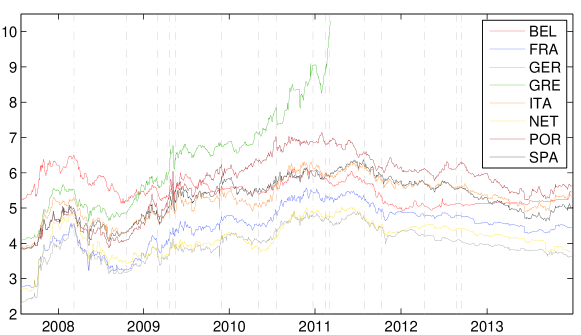
Figure 1: Daily evolution of Credit default swap spreads of eight European sovereigns, from July 21, 2008 to December 20, 2014 in log basis points. Vertical dashed lines represent major financial downturns: for a detailed description see Table 2.

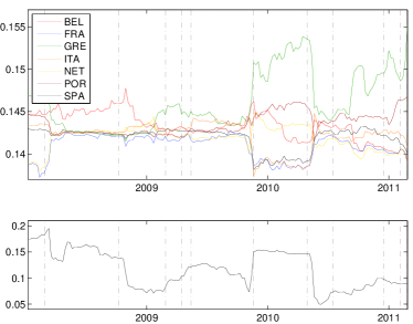
(a) Prior to the Greek crisis

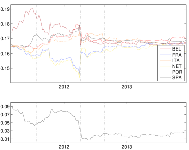
(b) After the Greek crisis

Figure 2: (Top panel): Shapley Value using the $SCoES$ at the $5\%$ level of Germany with respect to all the remaining countries. (Bottom panel): Overall risk of Germany measured by the $SCoES$ when all the remaining countries are in distress. Vertical dashed lines represent major financial downturns: for a detailed description see Table 2.

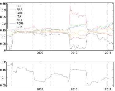
(a) Prior to the Greek crisis

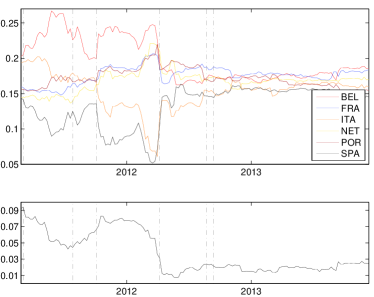
(b) After the Greek crisis

Figure 3: (Top panel): Banzhaf Value using the $SCoES$ at the $5\%$ level of Germany with respect to all the remaining countries. (Bottom panel): Overall risk of Germany measured by the $SCoES$ when all the remaining countries are in distress. Vertical dashed lines represent major financial downturns: for a detailed description see Table 2.

Moreover, to obtain results more robust to temporary short–term shocks affecting the considered economies, we consider weekly log–CDS returns. Specifically, at each point in time we estimate the $SCoES$ risk measure using a window of $N=26$ more recent weekly observations, and then we run the cooperative game to get the Shapley Value with $\tau_{1}=\tau_{2}=5\%$. It is worth mentioning that, with $p=8$ institutions, we are going to estimate $d=44\gg 26=N$ parameters. The Graphical–Lasso method of Friedman et al. (2008) delivers consistent estimates of the parameters even when the number of parameters is greater than the dimension of the sample, see Hastie et al. (2015) and Tibshirani (1996, 2011) for further details.
Results are reported in Figure 2, for the period before the onset of the Greek crisis (2a), as well as for the subsequent period (2b). For both periods, the bottom panel reports the overall impact of the distress of the remaining countries over the German economy as measured by the $SCoES$. Throughout the sample period, the overall risk of Germany due to the potential distress of one or more of the remaining European countries is high, until mid 2011. At that time, the level suddenly decreases to the lower level of about 0.09, as a consequence of the bailouts of Portugal and Greece, in May and July 2011, respectively. The overall risk still remain at the level of 0.09 till the April 2013 a few months later the announcement of the implementation of the of the Outright Monetary Transactions (OMT) and the European Stability Mechanism (ESM) in October 2012. If is worth noting that the launch of the first Long–Term Refinancing Operation (LTRO) by ECB in December 2011 and the second LTRO in March 2012 only had a moderate impact on the overall risk that decreased till mid 2012 and the unexpected strongest defence of the Euro of the ECB President Mario Draghi (July 26, 2012), did not contribute to reduce the risk of the Germany.
Concerning the evolution of the Shapley values reported in the top panel of Figure 2 and the Banzhaf Value in Figure 3, they can be interpreted as the normalised country risk factors. As expected, the two approaches provide different contributions to risk, in particular during the onset of the European crisis, reflecting their different properties. More precisely, the Shapley solution, suggests that, during the period in between the bailout of Ireland (November 29, 2010) and the bailout of Portugal (May 5, 2011), the most severe source of risk for the Germany’s economy is represented by the Greece, while Spain, Italy and France contribute less, see Figure 2. The picture by Banzhaf is a little bit different since, during the same period, the most important source of risk for Germany is Belgium, followed by Greece, a result which is a little bit surprisingly. Afterwards, the overall contributions of European countries converge, for both methods. The failure of the Greek austerity package in February 2012 suddenly increases the riskiness of Greece which is comparable only with that of Portugal at the beginning of 2011. Interestingly, the proposed approach is able to capture the most important events that happened during European sovereign debt crisis of 2012, as reported in Table 2.

6 Conclusions and further developments

This paper presents a cooperative game among distressed institutions to assess the potential damage done by all possible coalitions in distress. At this aim, a new risk measure which features some properties of the standard Expected Shortfall in a financial framework where some institutions are distressed and contagion threatens the remaining safe institutions is developed. Standard solution concepts like Shapley value and Banzhaf value can be helpful to measure the marginal contributions to systemic risk.
Our study of the European sovereign debt crisis of 2012 provides empirical support for the ability of the proposed cooperative Game approach to systemic risk measurement to effectively capture the dynamic evolution of the overall riskiness of the European countries. Furthermore, the proposed risk measurement framework is able to identify the major sources of risk and the risk contributions.
Further extensions of such a theoretical setup can be conceived, in terms of more complex and precise cost functions to be employed in the cooperative game. Moreover, a detailed analysis of correlations among distressed institutions might give rise to different game structures, such as a priori unions or bounded forms of cooperation which can be described with the help of graphs. In such cases, a model with some constraints might be necessary to determine the characteristics of risk transmission and the related consequences on the systemic risk. It is possible that a given structure with certain links among institutions can minimize the contagion risk.

Appendix

In this Appendix we provide analytical formulas for the computation of the $VaR$, $ES$, $SCoVaR$ and $SCoES$, as formally defined in the previous sections, under the assumption of the joint Gaussian distribution of the involved variables.

Proposition 16.

Let $X\sim\mathcal{N}_{p}\left(\mu,\Sigma\right)$ where $\mu\in\mathbb{R}^{p}$ is a vector of location parameters and $\Sigma$ is a $\left(p\times p\right)$– symmetric variance-covariance matrix. Consider the transformation $Z=\left[X_{i},\sum_{k=1,k\neq i}^{p}X_{k}\right]^{\prime}$, for $i=1,2,\dots,p$, then $Z\sim\mathcal{N}_{2}\left(\mu_{Z},\Sigma_{Z}\right)$, with

$$\mu_{Z} =\left[\mu_{i},\ \sum_{k=1,k\neq i}^{p}\mu_{k}\right]^{\prime}$$ (12)

$$\Sigma_{Z} =\left(\begin{matrix}\sigma^{2}(X_{i})&\sum_{k=1,k\neq i}^{p}\sigma_{i,k}\\ &&\\ \sum_{k=1,k\neq i}^{p}\sigma_{i,k}&\sigma^{2}\left(\sum_{k=1,k\neq i}^{p}X_{k}\right)\end{matrix}\right),$$ (13)

where $\sum_{k=1,k\neq i}^{p}\sigma_{i,k}$ denotes the covariance between $X_{i}$ and $\sum_{k=1,k\neq i}^{p}X_{k}$, and $\sigma^{2}(\cdot)$ denotes the variance of $X_{i}$. Under the previous assumptions the VaR, ES, of $X_{i}$, for $i=1,2,\dots,p$ are calculated as follows:

$$\widehat{\nu}_{i}^{\tau_{2}} \equiv VaR_{\tau_{2}}\left(\sum_{k=1,k\neq i}^{p}X_{k}\right)$$

$$=\sum_{k=1,k\neq i}^{p}\mu_{k}+\sqrt{\sigma^{2}\left(\sum_{k=1,k\neq i}^{p}X_{k}\right)}\Phi^{-1}\left(\tau_{2}\right)$$ (14)

$$\widehat{\psi}_{i}^{\tau_{2}} \equiv ES_{\tau_{2}}\left(\sum_{k=1,k\neq i}^{p}\mu_{k}\right)$$

$$=\sum_{k=1,k\neq i}^{p}\mu_{k}-\sqrt{\sigma^{2}\left(\sum_{k=1,k\neq i}^{p}X_{k}\right)}\dfrac{\phi\left(\widehat{\nu}_{i}^{\tau_{2}}\right)}{\Phi\left(\widehat{\nu}_{i}^{\tau_{2}}\right)},$$ (15)

see, Nadarajah et al. (2014) and Bernardi (2013), while the SCoVaR and SCoES becomes

$$\hat{\gamma}_{i|\sum_{k\neq i}X_{k}}^{\tau_{1}|\tau_{2}} \equiv SCoVaR_{i|\sum_{k\neq i}X_{k}}^{\tau_{1}|\tau_{2}}$$

$$:=y\in\mathbb{R}\ni\frac{F_{X_{i},\sum_{k\neq i}X_{k}}\left(y,\sum_{k=1,k\neq i}^{p}X_{k}\leq\widehat{\nu}_{i}^{\tau_{2}}\right)}{\tau_{2}}=\tau_{1}$$ (16)

$$\hat{\varsigma}_{i|\sum_{k=1,k\neq i}X_{k}}^{\tau_{1}|\tau_{2}} \equiv SCoES_{i|\sum_{k\neq i}}^{\tau_{1}|\tau_{2}}$$

$$=\sum_{k\neq i}^{p}\mu_{k}-\sqrt{\sigma^{2}\left(X_{i}\right)}\left[\phi\left(\hat{\gamma}_{i|\sum_{k\neq i}X_{k}}^{\tau_{1}|\tau_{2}}\right)\Phi\left(\frac{\widehat{\nu}_{i}^{\tau_{2}}-\rho\hat{\gamma}_{i|\sum_{k\neq i}X_{k}}^{\tau_{1}|\tau_{2}}}{\sqrt{1-\rho^{2}}}\right)\right.$$

$$\qquad\qquad\qquad\qquad\qquad\qquad\left.+\rho\phi\left(\widehat{\nu}_{i}^{\tau_{2}}\right)\Phi\left(\frac{\hat{\gamma}_{i|\sum_{k\neq i}X_{k}}^{\tau_{1}|\tau_{2}}-\rho\widehat{\nu}_{i}^{\tau_{2}}}{\sqrt{1-\rho^{2}}}\right)\right],$$ (17)

for $i=1,2,\dots,p$, where $F_{X,Y}\left(\cdot\right)$ denotes the joint cdf of the random variables $\left(X,Y\right)$.

Equation (16) implicitly defines the $SCoVaR$ as the value of $y$ that solves the conditional cdf of the involved variables equal to $\tau_{1}$. The solution always exists and is unique because the involved random variables are absolutely continuous.

References

- Abbasi and Hosseinifard (2013) Babak Abbasi and S. Zahra Hosseinifard. Tail conditional expectation for multivariate distributions: A game theory approach. Statistics & Probability Letters, 83(10):2228 – 2235, 2013. ISSN 0167-7152. doi: http://dx.doi.org/10.1016/j.spl.2013.06.012. URL http://www.sciencedirect.com/science/article/pii/S0167715213002174.
- Acerbi (2002) Carlo Acerbi. Spectral measures of risk: A coherent representation of subjective risk aversion. Journal of Banking & Finance, 26(7):1505 – 1518, 2002. ISSN 0378-4266. doi: http://dx.doi.org/10.1016/S0378-4266(02)00281-9. URL http://www.sciencedirect.com/science/article/pii/S0378426602002819.
- Acerbi and Tasche (2002) Carlo Acerbi and Dirk Tasche. Expected shortfall: A natural coherent alternative to value at risk. Economic Notes, 31(2):379–388, 2002. ISSN 1468-0300. doi: 10.1111/1468-0300.00091. URL http://dx.doi.org/10.1111/1468-0300.00091.
- Acharya et al. (2012) V.V. Acharya, R.F. Engle, and M. Richardson. Capital shortfall: a new approach to ranking and regulating systemic risks. American Economic Review, 102:59–64, 2012.
- Adrian and Brunnermeier (2011) T. Adrian and M.K. Brunnermeier. Covar. Working paper, 2011.
- Adrian and Brunnermeier (2016) Tobias Adrian and Markus K. Brunnermeier. Covar. American Economic Review, 106(7):1705–41, July 2016. doi: 10.1257/aer.20120555. URL http://www.aeaweb.org/articles?id=10.1257/aer.20120555.
- Altman and Hotchkiss (2010) Edward I Altman and Edith Hotchkiss. Corporate financial distress and bankruptcy: Predict and avoid bankruptcy, analyze and invest in distressed debt, volume 289. John Wiley & Sons, 2010.
- Anily and Haviv (2014) Shoshana Anily and Moshe Haviv. Subadditive and homogeneous of degree one games are totally balanced. Oper. Res., 62(4):788–793, August 2014. ISSN 0030-364X. doi: 10.1287/opre.2014.1283. URL http://dx.doi.org/10.1287/opre.2014.1283.
- Artzner et al. (1999) Philippe Artzner, Freddy Delbaen, Jean-Marc Eber, and David Heath. Coherent measures of risk. Mathematical finance, 9(3):203–228, 1999.
- Banzhaf III (1965) John F Banzhaf III. Weighted voting doesn’t work: A mathematical analysis. Rutgers L. Rev., 19:317, 1965.
- Benoit et al. (2016) Sylvain Benoit, Jean-Edouard Colliard, Christophe Hurlin, and Christophe Pérignon. Where the risks lie: A survey on systemic risk. Review of Finance, 2016. doi: 10.1093/rof/rfw026. URL http://rof.oxfordjournals.org/content/early/2016/06/01/rof.rfw026.abstract.
- Bernardi (2013) M. Bernardi. Risk measures for skew normal mixtures. Statistics & Probability Letters, 83:1819–1824, 2013.
- Bernardi and Catania (2015) Mauro Bernardi and Leopoldo Catania. Switching-gas copula models with application to systemic risk. arXiv preprint arXiv:1504.03733, 2015.
- Bernardi et al. (2016) Mauro Bernardi, Fabrizio Durante, Piotr Jaworski, Petrella Lea, and Gianfausto Salvadori. Conditional risk based on multivariate hazard scenarios. working paper, 2016.
- Billio et al. (2012) M. Billio, M. Getmansky, A.W. Lo, and L. Pellizon. Econometric measures of connectedness and systemic risk in the finance and insurance sectors. Journal of Financial Econometrics, 101:535–559, 2012.
- Bisias et al. (2012) Dimitrios Bisias, Mark Flood, Andrew W. Lo, and Stavros Valavanis. A survey of systemic risk analytics. Annual Review of Financial Economics, 4(1):255–296, 2012. doi: 10.1146/annurev-financial-110311-101754. URL http://dx.doi.org/10.1146/annurev-financial-110311-101754.
- Blasques et al. (2014) Francisco Blasques, Siem Jan Koopman, Andre Lucas, and Julia Schaumburg. Spillover dynamics for systemic risk measurement using spatial financial time series models. Tinbergen Institute Discussion Paper 14-107/III, 2014.
- Casajus (2014) André Casajus. The Shapley value without efficiency and additivity. Math. Social Sci., 68:1–4, 2014. ISSN 0165-4896. doi: 10.1016/j.mathsocsci.2013.12.001. URL http://dx.doi.org/10.1016/j.mathsocsci.2013.12.001.
- Cherubini and Mulinacci (2014) Umberto Cherubini and Sabrina Mulinacci. Contagion-based distortion risk measures. Appl. Math. Lett., 27:85–89, 2014. ISSN 0893-9659. doi: 10.1016/j.aml.2013.07.007. URL http://dx.doi.org/10.1016/j.aml.2013.07.007.
- Csóka and Pintér (2016) Péter Csóka and Miklós Pintér. On the impossibility of fair risk allocation. B. E. J. Theor. Econ., 16(1):143–158, 2016. ISSN 2194-6124. doi: 10.1515/bejte-2014-0051. URL http://dx.doi.org/10.1515/bejte-2014-0051.
- Csóka et al. (2007) Péter Csóka, P. Jean-Jacques Herings, and László Á. Kóczy. Coherent measures of risk from a general equilibrium perspective. Journal of Banking & Finance, 31(8):2517 – 2534, 2007. ISSN 0378-4266. doi: http://dx.doi.org/10.1016/j.jbankfin.2006.10.026. URL http://www.sciencedirect.com/science/article/pii/S0378426607000404.
- Csóka et al. (2009) Péter Csóka, P. Jean-Jacques Herings, and László Á. Kóczy. Stable allocations of risk. Games and Economic Behavior, 67(1):266 – 276, 2009. ISSN 0899-8256. doi: http://dx.doi.org/10.1016/j.geb.2008.11.001. URL http://www.sciencedirect.com/science/article/pii/S0899825608002042. Special Section of Games and Economic Behavior Dedicated to the 8th ACM Conference on Electronic Commerce.
- Denault (2001) Michel Denault. Coherent allocation of risk capital. Journal of risk, 4:1–34, 2001.
- Drehmann and Tarashev (2013) Mathias Drehmann and Nikola Tarashev. Measuring the systemic importance of interconnected banks. Journal of Financial Intermediation, 22(4):586 – 607, 2013. ISSN 1042-9573. doi: http://dx.doi.org/10.1016/j.jfi.2013.08.001. URL http://www.sciencedirect.com/science/article/pii/S1042957313000326.
- Einy and Haimanko (2011) Ezra Einy and Ori Haimanko. Characterization of the Shapley-Shubik power index without the efficiency axiom. Games Econom. Behav., 73(2):615–621, 2011. ISSN 0899-8256. doi: 10.1016/j.geb.2011.03.007. URL http://dx.doi.org/10.1016/j.geb.2011.03.007.
- Engle et al. (2014) Robert Engle, Eric Jondeau, and Michael Rockinger. Systemic risk in europe. Review of Finance, 2014. doi: 10.1093/rof/rfu012. URL http://rof.oxfordjournals.org/content/early/2014/03/29/rof.rfu012.abstract.
- Feltkamp (1995) Vincent Feltkamp. Alternative axiomatic characterizations of the Shapley and Banzhaf values. Internat. J. Game Theory, 24(2):179–186, 1995. ISSN 0020-7276. doi: 10.1007/BF01240041. URL http://dx.doi.org/10.1007/BF01240041.
- Friedman et al. (2008) Jerome Friedman, Trevor Hastie, and Robert Tibshirani. Sparse inverse covariance estimation with the graphical lasso. Biostatistics, 9(3):432–441, 2008. doi: 10.1093/biostatistics/kxm045. URL http://biostatistics.oxfordjournals.org/content/9/3/432.abstract.
- Girardi and Ergün (2013) G. Girardi and A.T. Ergün. Systemic risk measurement: Multivariate garch estimation of covar. Journal of Banking & Finance, 37:3169–3180, 2013.
- Hastie et al. (2015) Trevor Hastie, Robert Tibshirani, and Martin Wainwright. Statistical Learning with Sparsity: The Lasso and Generalizations. CRC Press, 2015.
- Hautsch et al. (2014) Nikolaus Hautsch, Julia Schaumburg, and Melanie Schienle. Financial network systemic risk contributions. Review of Finance, 2014. doi: 10.1093/rof/rfu010. URL http://rof.oxfordjournals.org/content/early/2014/03/24/rof.rfu010.abstract.
- Huang et al. (2012a) Xin Huang, Hao Zhou, and Haibin Zhu. Systemic risk contributions. Journal of Financial Services Research, 42(1):55–83, 2012a. ISSN 1573-0735. doi: 10.1007/s10693-011-0117-8. URL http://dx.doi.org/10.1007/s10693-011-0117-8.
- Huang et al. (2012b) Xin Huang, Hao Zhou, and Haibin Zhu. Assessing the systemic risk of a heterogeneous portfolio of banks during the recent financial crisis. Journal of Financial Stability, 8(3):193 – 205, 2012b. ISSN 1572-3089. doi: http://dx.doi.org/10.1016/j.jfs.2011.10.004. URL http://www.sciencedirect.com/science/article/pii/S1572308911000544. The Financial Crisis of 2008, Credit Markets and Effects on Developed and Emerging Economies.
- Kalkbrener (2005) Michael Kalkbrener. An axiomatic approach to capital allocation. Math. Finance, 15(3):425–437, 2005. ISSN 0960-1627. doi: 10.1111/j.1467-9965.2005.00227.x. URL http://dx.doi.org/10.1111/j.1467-9965.2005.00227.x.
- Koller and Friedman (2009) Daphne Koller and Nir Friedman. Probabilistic graphical models: principles and techniques. MIT press, 2009.
- Kountzakis and Polyrakis (2013) C. Kountzakis and I. A. Polyrakis. Coherent risk measures in general economic models and price bubbles. J. Math. Econom., 49(3):201–209, 2013. ISSN 0304-4068. doi: 10.1016/j.jmateco.2013.02.002. URL http://dx.doi.org/10.1016/j.jmateco.2013.02.002.
- Lucas et al. (2014) André Lucas, Bernd Schwaab, and Xin Zhang. Conditional euro area sovereign default risk. Journal of Business & Economic Statistics, 32(2):271–284, 2014. doi: 10.1080/07350015.2013.873540. URL http://dx.doi.org/10.1080/07350015.2013.873540.
- McNeil et al. (2015) Alexander J McNeil, Rüdiger Frey, and Paul Embrechts. Quantitative risk management: Concepts, techniques and tools. Princeton university press, second edition, 2015.
- Nadarajah et al. (2014) Saralees Nadarajah, Bo Zhang, and Stephen Chan. Estimation methods for expected shortfall. Quantitative Finance, 14(2):271–291, 2014. doi: 10.1080/14697688.2013.816767. URL http://dx.doi.org/10.1080/14697688.2013.816767.
- Owen (1995) Guillermo Owen. Game theory. Academic Press: New York, third edition, 1995.
- Ravikumar et al. (2011) Pradeep Ravikumar, Martin J. Wainwright, Garvesh Raskutti, and Bin Yu. High-dimensional covariance estimation by minimizing -penalized log-determinant divergence. Electron. J. Statist., 5:935–980, 2011. doi: 10.1214/11-EJS631. URL http://dx.doi.org/10.1214/11-EJS631.
- Shapley (1988) Lloyd S. Shapley. A value for -person games [from contributions to the theory of games, vol. 2, 307–317, Princeton Univ. Press, Princeton, NJ, 1953; MR 14, 779]. In The Shapley value, pages 31–40. Cambridge Univ. Press, Cambridge, 1988. doi: 10.1017/CBO9780511528446.003. URL http://dx.doi.org/10.1017/CBO9780511528446.003.
- Shapley and Shubik (1969) Lloyd S. Shapley and Martin Shubik. On market games. J. Econom. Theory, 1:9–25 (1970), 1969. ISSN 0022-0531.
- Sordo et al. (2015) Miguel A. Sordo, Alfonso Suárez-Llorens, and Alfonso J. Bello. Comparison of conditional distributions in portfolios of dependent risks. Insurance: Mathematics and Economics, 61:62 – 69, 2015. ISSN 0167-6687. doi: http://dx.doi.org/10.1016/j.insmatheco.2014.11.008. URL http://www.sciencedirect.com/science/article/pii/S0167668714001607.
- Stoica (2006) George Stoica. Relevant coherent measures of risk. J. Math. Econom., 42(6):794–806, 2006. ISSN 0304-4068. doi: 10.1016/j.jmateco.2006.03.006. URL http://dx.doi.org/10.1016/j.jmateco.2006.03.006.
- Tibshirani (1996) Robert Tibshirani. Regression shrinkage and selection via the lasso. J. Roy. Statist. Soc. Ser. B, 58(1):267–288, 1996. ISSN 0035-9246. URL http://links.jstor.org/sici?sici=0035-9246(1996)58:1<267:RSASVT>2.0.CO;2-G&origin=MSN.
- Tibshirani (2011) Robert Tibshirani. Regression shrinkage and selection via the lasso: a retrospective. J. R. Stat. Soc. Ser. B Stat. Methodol., 73(3):273–282, 2011. ISSN 1369-7412. doi: 10.1111/j.1467-9868.2011.00771.x. URL http://dx.doi.org/10.1111/j.1467-9868.2011.00771.x.
- Tsanakas (2009) Andreas Tsanakas. To split or not to split: Capital allocation with convex risk measures. Insurance: Mathematics and Economics, 44(2):268 – 277, 2009. ISSN 0167-6687. doi: http://dx.doi.org/10.1016/j.insmatheco.2008.03.007. URL http://www.sciencedirect.com/science/article/pii/S0167668708000425.
- Tsanakas and Barnett (2003) Andreas Tsanakas and Christopher Barnett. Risk capital allocation and cooperative pricing of insurance liabilities. Insurance Math. Econom., 33(2):239–254, 2003. ISSN 0167-6687. doi: 10.1016/S0167-6687(03)00137-9. URL http://dx.doi.org/10.1016/S0167-6687(03)00137-9. Papers presented at the 6th IME Conference (Lisbon, 2002).
- van den Brink and van der Laan (1998) René van den Brink and Gerard van der Laan. Axiomatizations of the normalized Banzhaf value and the Shapley value. Soc. Choice Welf., 15(4):567–582, 1998. ISSN 0176-1714. doi: 10.1007/s003550050125. URL http://dx.doi.org/10.1007/s003550050125.