Full-vortex flux qubit for charged particle optics

Abstract

We introduce a design of a superconducting flux qubit capable of holding a full magnetic flux quantum $\phi_{0}$, which arguably is an essential property for applications in charged particle optics. The qubit comprises a row of $N$ constituent qubits, which hold a fractional magnetic flux quantum $\phi_{0}/N$. Insights from physics of the transverse-field Ising chain reveal that properly designed interaction between these constituent qubits enables their collective behavior while also maintaining the overall quantumness.

I Introduction

Charged particle optics is a potentially fruitful, albeit lesser-known, application area of quantum science and technology. Among various proposals O-L-F (1, 2, 3), ideas of entanglement-enhanced electron microscopy (EEEM) eeem (4, 5) and molecule-by-molecule nano-fabrication q-interface (6) have been put forward. These latter schemes employ superconducting qubits Superconducting qubits (7), which generally produce quantum mechanically superposed electromagnetic potentials around them. Consequently, a charged particle flying nearby gets entangled with the qubit. For instance, EEEM would utilize such entanglement to image fragile biological molecules with a much-needed signal-to-noise ratio beyond the standard quantum limit under the condition of a limited allowable number of electrons looping electron scheme (8).

Magnetic flux qubits are preferable to charge qubits especially when medium or high energy charged particles are used. A closed ring of magnetic flux quantum $\phi_{0}=h/2e$ is particularly useful okamoto-nagatani (5, 6) because the full phase shift $\pi$ is induced on the single-charged matter wave going through the ring via the Aharonov-Bohm (AB) effect AB effect (9, 10), irrespective of the kinetic energy or the mass of the particle, while applying effectively zero classical force to it. A device that naturally comes to mind for generating a superposition of the presence and absence of a magnetic flux is the rf-SQUID qubit rf-SQUID qubit exp (11), which can be put in a quantum mechanically superposed state of two opposing shielding currents with a suitably adjusted external magnetic field. Furthermore, a way to make the trapped magnetic flux circular has also been put forward okamoto-nagatani (5). As shown below, however, on close examination one finds practical difficulties associated with this simple idea, despite its soundness at the conceptual level.

II Difficulties with a single rf-SQUID

We begin by listing several definitions. Let the critical current of the Josephson junction (JJ), which interrupts the loop inductor $L$ of an rf-SQUID, be $i_{c}$. The effective capacitance, which include the effect of stray capacitance, is denoted by $C$. Define $E_{J}=i_{c}\phi_{0}/2\pi$, $E_{C}=\left(2e\right)^{2}/2C$ and $\beta=2\pi Li_{c}/\phi_{0}$. Let the magnetic flux threading $L$ be $\phi+\phi_{0}/2+\phi_{err}$, where the first term is generated by the current in the inductor $L$, while $\phi_{0}/2+\phi_{err}$ represents the externally applied bias magnetic flux. Although the bias magnetic flux is ideally $\phi_{0}/2$, an error $\phi_{err}$ is unavoidable. The potential energy $U\left(\phi\right)=\phi^{2}/2L+E_{J}\cos\left[2\pi\left(\phi+\phi_{err}\right)/\phi_{0}\right]$ has two minima with the difference $\Delta\phi$ (see Fig. 1). Henceforth we assume $\phi_{err}=0$ unless stated otherwise. It is a unique character of charged particle optics applications that $\Delta\phi$ should be close to $\phi_{0}$. The potential curve $U\left(\phi\right)$ is shown in Fig. 1. It can be shown that $\Delta\phi\cong\phi_{0}/\left(1+\beta^{-1}\right)$ for $\Delta\phi\cong\phi_{0}$ and hence a large $\beta$ is needed to keep $\Delta\phi$ close to $\phi_{0}$ (See Appendix A).

Consider EEEM for example eeem (4, 5). In transmission electron microscopy (TEM), the lateral size of the coherent electron wavefront is typically of the order of ${l_{C}\cong 10\>\mu\mathrm{m}}$ Tonomura AB (10). The beam divergence in TEM vary, but it can be less than ${\theta_{d}\cong 100\>\mu\mathrm{rad}}$ in experimental configurations such as Lorenz TEM Lorenz TEM (12). This suggests that the size of the qubit along the optical axis needs to be smaller than ${l_{C}/\theta_{d}\cong 10\>\mathrm{cm}}$ to keep the beam inside the qubit, and hence the size should be a few $\mathrm{cm}$ at most. (The size of the qubit along the axis perpendicular to the optical axis should be ${l_{C}\cong 10\>\mu\mathrm{m}}$.) For rough estimation purposes, we compute the inductance of the rf-SQUID using the formula $L\cong\mu_{0}l/2\pi$ for the coaxial cable, neglecting the logarithmic factor. This results in a value of, e.g., ${L=5\>\mathrm{nH}}$ when ${l\cong 2.5\>\mathrm{cm}}$. This value will turn out to be too small.

We show why a single rf-SQUID qubit does not work in practice. Suppose that we have $\beta=2\pi Li_{c}/\phi_{0}\cong 10\gg 1$ to make $\Delta\phi\cong\phi_{0}$. Then, the critical current of the JJ needs to be ${i_{c}=500\>\mathrm{nA}}$, assuming the above value ${L=5\>\mathrm{nH}}$. This implies a large tunnel barrier $\cong 2E_{J}\propto i_{c}$ (See Appendix A) between the two fluxoid states. Hence, a question is whether we have a sufficiently high rate of tunneling between the two fluxoid states. The state-of-the-art JJ with ${i_{c}=500\>\mathrm{nA}}$ could have a junction capacitance $C_{J}$ as small as ${1\>\mathrm{fF}}$. If this is the capacitance governing the system, our numerical calculation (See Appendix A) gives an energy splitting of the size ${\Delta\cong 1\>\mu\mathrm{eV}}$. However, $\Delta$ is sensitive to stray capacitance: For example, having ${C=10\>\mathrm{fF}}$ dramatically suppresses the quantum tunneling effect, resulting in miniscule energy splitting $\Delta$ smaller than ${30\>\mathrm{pV}}$. (Calculations using the WKB approximation overestimates $\Delta$.) Such a qubit is not operable because then ${h/\Delta>100\>\mu\mathrm{s}}$ corresponds to e.g. the largest known decoherence time of superconducting qubits. This lack of robustness is especially problematic in our case of the large-size rf-SQUID. Analysis suggests that the loop size of a few cm could result in a stray capacitance as large as several hundred ${\mathrm{fF}}$ (See Appendix B).

Qubit decoherence is not the only problem with a miniscule $\Delta$. This demands a precise alignment of the energy level of the two lowest potential wells by the external bias flux, because a misalignment larger than $\Delta$ results in localization of the otherwise symmetric ground state to one potential well, while the anti-symmetric first excited state is localized to the other. Such localization is detrimental to charged particle optics applications okamoto-nagatani (5, 6). The energy difference between the two lowest potential wells is $E_{err}\cong\left(\phi_{0}/L\right)\phi_{err}$ if $\beta\gg 1$, when the bias magnetic flux $\phi_{0}/2$ has a small additional error $\phi_{err}$ (See Appendix A). Since the accuracy of the bias flux must satisfy ${E_{err}<\Delta<30\>\mathrm{peV}}$, a necessary condition $\phi_{err}<10^{-9}\phi_{0}$ must be met.

The above condition $\phi_{err}<10^{-9}\phi_{0}$ is difficult to satisfy. First, a recent experimental study in the context of quantum computing finds flux noise in a “coupler loop”, with a $1/f^{0.91}\cong 1/f$ form of power spectral density, of the order of $S_{n}=\phi_{n}^{2}/f=\left(10^{-5}\phi_{0}\right)^{2}/f$, where $f$ is the frequency MIT annealer (13). The variance of the flux noise in a bandwidth between $f_{L}$ and $f_{H}$ is computed to be, using a well-known relation, $\int_{\omega_{L}}^{\omega_{H}}S_{n}d\omega/\pi=2\int_{f_{L}}^{f_{H}}\left(\phi_{n}^{2}/f\right)df=\left(2\phi_{n}^{2}/\pi\right)\ln\left(f_{H}/f_{L}\right)\cong\phi_{n}^{2}$, where we neglected the logarithmic factor and the numerical factor $2/\pi$ in the last step. The flux fluctuation is thus of the order of $10^{-5}\phi_{0}$ in this context. A similar value was reported also in another experiment Harris coupled rf-SQUIDs (14). Second, analysis of macroscopic resonant tunneling (MRT) allows us to estimate flux noise both at low and high frequencies MRT noise measurements (15). In particular, the low frequency studies suggest that the noise is of the order of $\left(10^{-3}\sim 10^{-4}\right)\phi_{0}$ MRT comment (16). Third, the noise in the output of a SQUID magnetometer, which must be larger than the magnetic noise in the environment, should therefore give an upper bound of the environmental noise. (The noise, in terms of magnetic flux density, is typically found smaller with a larger effective area of the magnetometer SQUID (17), suggesting that the intrinsic noise of the SQUID plays a role.) A recent study SQUID (17) reports flux noise power density of $\sqrt{S_{n}}=\left(0.09\>\mathrm{fT}/\sqrt{\mathrm{Hz}}\right)\left\{1+\left(300\>\mathrm{Hz}/f\right)^{0.3}+\left(3\>\mathrm{Hz}/f\right)\right\}$. Integrating this from ${f_{L}=0.1\>\mathrm{Hz}}$ to ${f_{H}=10\>\mathrm{GHz}}$ for example, we obtain the variance of magnetic flux noise $\int_{\omega_{L}}^{\omega_{H}}S_{n}d\omega/\pi\cong\left(1\>\mathrm{pT}\right)^{2}$. Multiplying the aforementioned qubit area of the order of ${l_{C}\times 1\>\mathrm{cm}}$, we obtain the amplitude of the magnetic flux noise of the order of ${10^{-19}\>\mathrm{Wb}\cong 10^{-4}\phi_{0}}$, most of which comes from the frequency independent term. Fourth, if we crudely model the electromagnetic environment (i.e. the metallic container of the qubit etc.) as a single inductor $L_{EM}$, there should be thermal magnetic noise $\phi_{n}$ according to the relation $\phi_{n}^{2}/2L_{EM}\cong k_{B}T/2$. For example, values ${T=100\>\mathrm{mK}}$ and ${L_{EM}=100\>\mathrm{nH}}$ results in $\phi_{n}\cong 0.18\phi_{0}$. Hence the magnetic coupling between the qubit and $L_{EM}$ must be very small. The above four findings, when taken together, strongly suggest that $\phi_{err}<10^{-9}\phi_{0}$ is quite unattainable in practice.

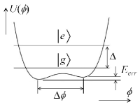
Figure 1: Potential curve $U\left(\phi\right)$ of a single rf-SQUID. Energy levels of the ground state $|g\rangle$ and the excited state $|a\rangle$ are shown for a device with a strong quantum effect, i.e. ${C=10\>\mathrm{fF}}$, ${L=800\>\mathrm{pH}}$ and $\beta=1.11$. The bias energy $E_{err}$ between the wells is exaggerated in the figure. The energy levels are computed assuming $E_{err}=0$.

III Proposed solution

A solution to the above problem is to combine $N>1$ rf-SQUIDs, where each rf-SQUID is associated with a magnetic flux difference $\Delta\phi=\phi_{0}/N$ between the two fluxoid states. Specifically, we consider $N=4$. An rf-SQUID with $\beta=\sqrt{2}\pi/4\cong 1.11$ has the desired difference $\Delta\phi=\phi_{0}/4$. (A simple analysis shows that an error of $1\%$ in $\beta$ corresponds to an error of $4\%$ in $\Delta\phi$. The expression for $E_{err}$ is modified to be $E_{err}\cong\left(\phi_{0}/4L\right)\phi_{err}$, when $\Delta\phi=\phi_{0}/4$.) Our strategy of using multiple rf-SQUIDs may seem simple, but all $N$ SQUIDs should work together, preferably without using the entire machinery of a universal quantum information processor.

For definiteness, let the inductance $L$ of the rf-SQUIDs be ${800\>\mathrm{pH}}$. This inductance value suggests a size ${l\cong 4\>\mathrm{mm}}$ if we employ the aforementioned formula $L\cong\mu_{0}l/2\pi$. (Further discussion on estimating $L$ is given at the end of this section.) Our analysis described in Appendix B suggests that the effective junction capacitance $C$, mostly coming from stray capacitance, could be as large as ${60\>\mathrm{fF}}$, but certain measures, such as etching of silicon inside the inductor loop, $could$ bring this down to about ${3\>\mathrm{fF}}$. Numerical analysis of a single rf-SQUID shows ample ${\Delta=\left(67\pm 3\right)\>\mu\mathrm{eV}}$ if ${C=10\>\mathrm{fF}}$ (see Appendix A, where we assumed $1\%$ uncertainty in the values of $\alpha$ and $\beta$). Figure 1 shows this case. In the case of ${C=100\>\mathrm{fF}}$, we obtain ${\Delta=\left(7.9\pm 0.5\right)\>\mu\mathrm{eV}}$ (again with $1\%$ uncertainty in $\alpha$ and $\beta$), which may still be acceptable and shows certain degree of robustness of the energy splitting $\Delta$. (Possibly, a moderately large $C$ may even be advantageous because then the flux $\phi$ is well-localized. See Sec. V along with Appendix E for the effect of quantum mechanically uncertain $\phi$.)

In practice, device parameters vary from one JJ to another. To achieve small spread in device parameters among multiple rf-SQUIDs, the use of the compound JJ (CJJ), which is effectively a JJ with adjustable $i_{c}$, will likely be necessary compound JJ (18). To uniformly modulate the parameters of multiple rf-SQUIDs during operation (see Sec. VI), the more complex compound-CJJ (CCJJ) may be needed compound-compound JJ (19). In the rest of this paper, the term “JJ” will mean effective JJ that may actually be CJJ or CCJJ.

We consider a 1-dimensional (1D) chain of $N=4$ rf-SQUIDs, along which charged particles fly. These rf-SQUIDs work together as a single qubit, which we will call the composite qubit. For the moment, we regard each rf-SQUID as a spin $1/2$, labeled consecutively as $k=1,2,\cdots,N$. Let the $k$-th spin’s basis states be $\mid\uparrow\rangle_{k}$ and $\mid\downarrow\rangle_{k}$, which correspond to the two fluxoid states of the $k$-th rf-SQUID. Define symmetric and antisymmetric states respectively as $|s\rangle_{k}=\left(\mid\uparrow\rangle_{k}+\mid\downarrow\rangle_{k}\right)/\sqrt{2}$ and $|a\rangle_{k}=\left(\mid\uparrow\rangle_{k}-\mid\downarrow\rangle_{k}\right)/\sqrt{2}$. For charged particle optics applications, the ground state of noninteracting spins $\otimes_{k=1}^{N}|s\rangle_{k}$ is useless. The basis states of the composite qubit should instead be the “ferromagnetic” $\mid\Uparrow\rangle=\otimes_{k=1}^{N}\mid\uparrow\rangle_{k}$ and $\mid\Downarrow\rangle=\otimes_{k=1}^{N}\mid\downarrow\rangle_{k}$. We will show that suitable ferromagnetic interaction between the spins gives what we want. The low-lying energy eigenstates should essentially be $\left(\mid\Uparrow\rangle\pm\mid\Downarrow\rangle\right)/\sqrt{2}$ because of tunneling between the states $\mid\Uparrow\rangle$ and $\mid\Downarrow\rangle$, which does occur since $N$ is finite in our case. Many methods to couple flux qubits have been studied and demonstrated, including tunable ones JJ coupling (20).

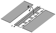
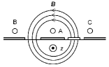
(a)                (b)

Figure 2: (a) Proposed device structure comprising a row of $N=4$ rf-SQUIDs on a surface of a substrate. Each “cross” symbol represents a compound JJ in an abbreviated way. Charged particles fly in close proximity to, and in parallel with, the surface along the $z$ axis. Superconducting planes (shaded parts) are placed so that the field lines of magnetic flux density $\mathbf{\boldsymbol{\mathbf{\mathit{B}}}}$ are forced to make a loop. Adjacent rf-SQUIDs interact through couplers, which are represented by hatched blocks. Flux biasing coils, possibly using persistent current trapping persistent current trapping (21), are not shown. (b) The cross section of the device, perpendicular to the optical axis $z$. The charged particle beam A goes through the magnetic flux ring, whereas the beams B and C do not. The white box represents an rf-SQUID, while shaded boxes represent superconducting films. The shape of the field lines is only schematic. See the main text for further discussions on the shape of the magnetic flux ring.

Figure 2 illustrates a possible implementation of the composite qubit. A row of $4$ rf-SQUIDs are placed on a substrate as shown in Fig. 2 (a). Charged particles fly along the optical $z-$axis. Each rf-SQUID is biased with an external flux $\phi_{0}/2$, either by an additional coil or by persistent-current-trapping persistent current trapping (21). Either way, care should be taken to avoid known difficulties in biasing an rf-SQUID qubit Ralph et al (22, 23) and known methods should be employed as needed to take care of cross coupling between bias controls JJ coupling (20). Adjacent rf-SQUIDs interact ferromagnetically through a coupling circuit. These rf-SQUIDs are arranged with suitably grounded superconducting strips in such a way that the magnetic field from each rf-SQUID primarily makes a loop shown. The geometric design should be such that the field does not go sideways, i.e. to the adjacent rf-SQUIDs. At the same time, these superconducting strips, especially the one on the side of JJs, should be carefully designed so that they do not contribute much stray capacitance. Figure 2 (b) shows a cross section, perpendicular to the $z-$axis, of the device. A nominal phase difference $0$ or $\pi$ is produced between the charged particle wave going through the magnetic flux ring (A) and the waves passing by the ring (B and C), depending on the qubit state. These beams A, B, and C may be generated using a stencil mask in the upstream of the charged particle beam. It should be easy to envision using techniques in the field of microelectromechanical systems (MEMS) to, for example, make a groove where the beam A goes, etc.

Further consideration is warranted on the estimation of the loop inductance $L$. The magnetic energy stored in an inductor is

$$\frac{1}{2\mu_{0}}\int\boldsymbol{B}^{2}dV=\frac{1}{2L}\left\{\int\boldsymbol{B}\cdot d\boldsymbol{S}\right\}^{2},$$ (1)

in the case of a single-turn coil without magnetic material. Hence $L=\mu_{0}\left\{\int\boldsymbol{B}\cdot d\boldsymbol{S}\right\}^{2}/\int\boldsymbol{B}^{2}dV$, in which the magnetic flux density$\boldsymbol{B}$ may be replaced with any vector field that is proportional to $\boldsymbol{B}$, is determined entirely by the shape of magnetic field lines. For example, one may use the inductance formula for coaxial cables if the magnetic flux lines have the tight tube-like shape. Such a shape can in principle be formed by suitably placing coaxial superconducting tubes around the rf-SQUID. However, an application at hand may allow for more extended magnetic field distributions. For the example shown in Fig. 2 (b), the electron beams are only at positions A, B, and C and the magnetic field lines do not have to be tightly held together above the beam positions. In such cases, $L$ is larger for a similar size of rf-SQUIDs. As an extreme example, numerical analysis using InductEX software shows that a superconducting rectangular loop, with the width of ${10\>\mu\mathrm{m}}$ containing magnetic flux, on a flat substrate without any other superconducting part, has an inductance per unit length of $\cong{1.2\>\mathrm{nH/mm}}$ inductEX (24). This value is significantly larger than the case of a coaxial cable, where $\mu_{0}l/2\pi={0.2\>\mathrm{nH/mm}}$.

IV The Lagrangian

We model ferromagnetic interaction between neighboring rf-SQUIDs produced by the coupler circuits. For simplicity, we ignore boundary effects at both the ends of the chain. Let $L$ and $M$ respectively be the self inductance common to all the rf-SQUIDs and the effective mutual inductance common to all the neighboring pairs of rf-SQUIDs. The magnetic flux in the $k-$th rf-SQUID is $\phi_{k}+\phi_{0}/2$, where $\phi_{0}/2$ is the bias flux. Under a condition $M/L\ll 1$, a straightforward analysis (See Appendix C) shows that the magnetic energy stored in the system is $U_{mag}\cong\left[1/2\left(L+2M\right)\right]\sum_{k=1}^{N}\phi_{k}^{2}+\left(M/2L^{2}\right)\sum_{k=1}^{N-1}\left(\phi_{k+1}-\phi_{k}\right)^{2}$, to the first order in $M/L$. Henceforth we will use the above expression as if it is exact. To set up the Lagrangian $\hat{L}$ of the system, we define $\theta_{k}=2\pi\phi_{k}/\phi_{0}$, the gauge-invariant phase difference across the $k$-th JJ plus $\pi$, which we take as dynamical variables. The charging energy of the JJ capacitance gives the kinetic energy because it involves $\dot{\theta}_{k}=d\theta_{k}/dt$. On the other hand, the potential energy is stored in the inductors and the JJs. We obtain

$$\hat{L}=\sum_{k=1}^{N}\left\{\frac{C\phi_{0}^{2}}{2}\left(\frac{\dot{\theta}_{k}}{2\pi}\right)^{2}-\frac{M\phi_{0}^{2}}{2L^{2}}\left(\frac{\theta_{k+1}-\theta_{k}}{2\pi}\right)^{2}-E_{J}\cos\theta_{k}-\frac{\phi_{0}^{2}}{2\left(L+2M\right)}\left(\frac{\theta_{k}}{2\pi}\right)^{2}\right\}.$$ (2)

The Lagrangian (2) equivalently describes coupled inverted mechanical pendulums with a restoration force (the last term). We use this mechanical analog to aid our intuition. These pendulums are independent without interaction ($M/L\rightarrow 0$). Discretizing the quantum state space, we say that if the $k$-th pendulum is in the stable state $\theta_{k}<0$, then it is in the down state $\mid\downarrow\rangle_{k}$ and likewise the stable $\theta_{k}>0$ corresponds to $\mid\uparrow\rangle_{k}$. Note that all pendulums would effectively act as a single object and the ground state would be the desired entangled state $\left(\mid\Uparrow\rangle+\mid\Downarrow\rangle\right)/\sqrt{2}$ if the couplings among the pendulums are sufficiently strong. However, the mass and the energy barrier height for the group of pendulums are $N$ times those of the individual pendulum and quantum tunneling would be strongly suppressed. Consequently, a problem arises as to whether the decoherence time is longer than the time scale associated with the energy splitting and if the required accuracy of the bias magnetic flux is attainable. Our central question is whether there exists an intermediate coupling strength, where both the entangled ground state and sufficiently strong quantum fluctuation are realized.

V Many-body physics governing the system

Instead of calculating properties of the set of $4$ rf-SQUIDs by brute-force, we intend to gain broad physical insights from known many-body physics. Hence, despite that the number of rf-SQUIDs we consider is only $N=4$, we approximate it by infinity. We regard the composite qubit as a set of interacting spins. Our strategy is to see how the system changes upon renormalization: If the “quantumness” is kept upon renormalization, then we have evidence that $N$ rf-SQUIDs as a whole, or less precisely the “single renormalized rf-SQUID”, would keep desired overall quantumness. The “bare” parameters in renormalization theory correspond to the device parameters of the individual rf-SQUID.

Our model is described by the Hamiltonian Harris coupled rf-SQUIDs (14)

$$H=-J\sum_{i}\sigma_{i}^{z}\sigma_{i+1}^{z}-h\sum_{i}\sigma_{i}^{x}-\varepsilon\sum_{i}\sigma_{i}^{z},$$ (3)

where $\sigma$s are the Pauli matrices pertaining to the spins discussed above. This is the 1D transverse-field Ising model if $\varepsilon=0$, which has been extensively studied as a prototypical model to study quantum phase transitions Transverse Ising RG (25) and has also attracted much attention recently in the context of quantum annealing quantum annealing (26). The last term in Eq. (3), which is assumed to be small, is added to account for non-ideal flux biasing. Appropriate assignments of the variables are seen to be $J=M\phi_{0}^{2}/2N^{2}L^{2}$, $h=\Delta/2$ and $\varepsilon=E_{err}/2$ to map to the rf-SQUID case. The massive sine-Gordon model may seem more accurate, but aside from solvability the classical soliton size $\cong\sqrt{J/E_{J}}$ turns out to be small in the parameter region of interest, justifying the use of a spin-based model.

First, we examine the overall behavior. It is known that the ground state is ferromagnetic or paramagnetic if $R=h/J<1$ or $R>1$ respectively Transverse Ising RG (25). We note that a similar superposed ferromagnetic state has been observed experimentally in a system comprising $8$ flux qubits PRX experiment (27). It is also known that $R$ evolves according to a simple rule $R^{\prime}=R^{2}$ upon block renormalization of 2 spins Fernandez-Pacheco (28). This rule is robust as long as $\varepsilon$ is small (See Appendix D). This shows that the overall system behaves similarly to the constituent spins, or the rf-SQUIDs, if the system is near the quantum critical point (QCP) $R=1$. We introduce $\kappa=R-1$ to indicate the distance from the QCP.

The composite qubit must have two basis states by definition. The basis states $\mid\Uparrow^{\prime}\rangle$ and $\mid\Downarrow^{\prime}\rangle$ should respectively be similar to the totally polarized states$\mid\Uparrow\rangle$ and $\mid\Downarrow\rangle$, in the sense that they induce well-defined phase shifts differing by $\pi$ to the charged particle wave. A natural condition for any such basis state $|b\rangle$ is that the 2-point spin correlator $C\left(n\right)=\langle b|\sigma_{i}^{z}\sigma_{i+n}^{z}|b\rangle$ is close to $1$, for all positive $n$ smaller than the size of the spin chain $N$. Conversely, if a state satisfies this condition, then the state must be similar to either $\mid\Uparrow\rangle$, $\mid\Downarrow\rangle$ or their superposition. It is known in the case of an infinite chain at $\varepsilon=0$ that, at zero temperature (i.e. with a ground state) and also in the limit $n\rightarrow\infty$, $C\left(n\right)=\left(2\pi^{2}n^{2}\kappa\right)^{-1/4}e^{-n\kappa}$ if $\kappa>0$ (the paramagnetic phase) and $C\left(n\right)=\left(2\left|\kappa\right|\right)^{1/4}$ if $\kappa<0$ (the ferromagnetic phase) Transverse Ising RG (25). Under the condition $\kappa<0$, the polarization of spins over the entire infinite chain is $\langle b|\sigma_{i}^{z}|b\rangle=\sqrt{C\left(n\right)}=\left(2\left|\kappa\right|\right)^{1/8}$. However, we expect stronger polarization over a finite length, especially when the length is shorter than the average size of the “magnetic domain”. In the paramagnetic region $\kappa>0$, no polarization over the entire infinite chain is present. However, within a finite distance we still have polarization, e.g. $C\left(n\right)\varpropto\kappa^{1/4}$ at $n\cong 1/\kappa$, and hence our finite system could essentially be fully polarized for a small enough $\kappa$. Hence, the composite qubit might work also in the $\kappa>0$ region.

Despite the above remark on stronger polarization over a finite length, here we proceed conservatively. We require a $\kappa$ value, corresponding to the polarization $P$ of the infinite chain, to be sufficiently close to the full value $1$. From the perspective of charged particle optics, the two basis states of the composite qubit should have magnetic flux difference close to $\phi_{0}$. This does not necessarily mean that $P$ needs to be close to $1$ because the magnetic flux difference can also be adjusted by modestly varying $\beta$. (For example, $\beta=2\pi/3\sqrt{3}\cong 1.21$ would give the nominal flux difference $4\phi_{0}/3$.) However, a small value of $P$ generally means larger quantum uncertainty in the value of magnetic flux, which entails unwanted entanglement with a charged particle that could lead to excitation of the composite qubit. Although evaluation of such effects is a complex problem that is beyond the scope of the present work (See Appendix E for a preliminary analysis for EEEM), it is reasonable to assume that a value of $P$ close to $1$ should limit the size of aforementioned quantum uncertainty. Hence, for the sake of rough estimation, we assume $P=\left|\kappa\right|^{1/8}$ so that we obtain the full polarization $P=1$ at $\kappa=-1$, i.e. $R=0$. This conservative relation underestimates the known polarization $\langle b|\sigma_{i}^{z}|b\rangle=\left(2\left|\kappa\right|\right)^{1/8}$ near the QCP. For example, values of $P=0.90$ and $0.80$ respectively correspond to values of $R=0.57$ and $0.83$ because of the relation $R=1-P^{8}$.

To be specific, we analyze the case of $R<1$. We slightly extend the block renormalization scheme Fernandez-Pacheco (28) for the transverse-field Ising model to the case where a weak but non-zero longitudinal field is present (See Appendix D). Upon replacing each block of 2 spins with a renormalized spin, renormalized Hamiltonian parameters are obtained as

$$J^{\prime}=\frac{1}{\sqrt{1+R^{2}}}J,\>h^{\prime}=\frac{R}{\sqrt{1+R^{2}}}h,$$

$$\varepsilon^{\prime}=\left\{1+\frac{1+2R^{2}}{\left(1+R^{2}\right)^{3/2}}\right\}\varepsilon.$$ (4)

To be on the safe side, we assumed that the flux biasing errors $\varepsilon$ are with the same sign and magnitude for all rf-SQUIDs, although in reality we expect random biasing errors. To maintain quantumness, $h$ should not decrease too quickly upon renormalization in the region $h<J$. Although making $h$ close to $J$ minimizes the rate of decrease, this entails a smaller polarization $P$ and hence a compromise should be made. At the same time, $\varepsilon$ should not grow to exceed $h$ because of the analogous relation $E_{err}<\Delta$ in the case of the rf-SQUID. Equations (4) imply that both $J$ and $h$ grow proportional to $1/\sqrt{N}$ compared to the initial values, and similarly $\varepsilon\propto N^{\ln\left[\left(3+2\sqrt{2}\right)/2\sqrt{2}\right]/\ln 2}\cong N^{1.0}$ at the QCP.

Numerical calculations away from the QCP show the followings (See Appendix F). After $2$ iterations of block renormalization, implying that $N=2^{2}=4$ spins are combined to make a renormalized spin, the parameters $h$ and $\varepsilon$ evolve into renormalized values $h^{\prime\prime}$ and $\varepsilon^{\prime\prime}$ that depend on the initial value of $R$. For the aforementioned two values $R=0.57$, $0.83$ and the QCP value $R=1.0$, we respectively obtain $\left(h^{\prime\prime}/h\right)/\left(\varepsilon^{\prime\prime}/\varepsilon\right)=0.036$, $0.083$ and $0.12$. Hence the ratio $h/\varepsilon$ decreases by $1\sim 2$ orders of magnitude upon renormalization, implying that the original, constituent rf-SQUIDs must satisfy $10^{2\sim 3}E_{err}\cong\Delta$ in order to have a margin of an order of magnitude. For the parameters mentioned before, i.e. ${L=800\>\mathrm{pH}}$, ${C=10\>\mathrm{fF}}$, and $\beta=1.11$, the bias flux error must satisfy $\phi_{err}<10^{-\left(4\sim 5\right)}\phi_{0}$. The requirement will be an order of magnitude more stringent in the case of larger stray capacitance ${C=100\>\mathrm{fF}}$. Discussions in Sec. II suggests that the requirement $\phi_{err}<10^{-\left(4\sim 5\right)}\phi_{0}$ does not seem to be out of the realm of feasibility, although we must strive to minimize stray capacitance. Nonetheless, we have consistently been on the safe side and hence the biasing precision requirement may well be relaxed. Also note that the precision requirement is exponentially harder, and hence virtually impossible to satisfy, if we use a single large rf-SQUID qubit instead of the proposed composite qubit. Since the rf-SQUID coil has the inductance ${L=800\>\mathrm{pH}}$ with the size ${l\cong 4\>\mathrm{mm}}$ using the aforementioned formula $L\cong\mu_{0}l/2\pi$, the entire size of $N=4$ rf-SQUIDs is ${4l\cong 16\>\mathrm{mm}}$. This is well within the required length of a few $\mathrm{cm}$ mentioned in Sec II.

VI Operation of the composite qubit

Both in EEEM and non-invasive charge detection, we start with resetting the qubit in the state $\left(\mid\Uparrow^{\prime}\rangle+\mid\Downarrow^{\prime}\rangle\right)/\sqrt{2}$. This is done by, first setting all the rf-SQUID in the symmetric ground state when they are uncoupled at a large $R$. Then we go through the QCP adiabatically and reach the operation point such as $R=0.57$. In the infinite chain, the excitation gap is known to vanish at the QCP Transverse Ising RG (25) and the ground level is degenerate when $R<1$, but our system is finite. In order to roughly estimate the energy difference between the ground state and the excited state of the qubit, we use the renormalized version of $\Delta=2h$, which is the $2$-times renormalized parameter $\Delta^{\prime\prime}=2h^{\prime\prime}=0.31h=0.15\Delta={1.6\times 10^{-24}\>\mathrm{J}}$ (See Table AI of Appendix A), where we used the value $h^{\prime\prime}/h=0.153$ at $R=0.57$ (See Appendix F). Hence we need to take the time larger than $h/\Delta^{\prime\prime}={0.40\>\mathrm{ns}}$ to reach the operation point, where the qubit interacts with the charged particles. Then we either wait, so that the qubit state rotates about the axis of the Bloch sphere connecting the points $\left(\mid\Uparrow^{\prime}\rangle\pm\mid\Downarrow^{\prime}\rangle\right)/\sqrt{2}$, or apply a tiny additional flux to the biasing flux to rotate the state about the axis connecting $\mid\Uparrow^{\prime}\rangle$ and $\mid\Downarrow^{\prime}\rangle$ non-microwave control of qubits (29). Finally, the composite qubit is measured, for example magnetically, with respect to the basis states $\mid\Uparrow^{\prime}\rangle$ and $\mid\Downarrow^{\prime}\rangle$. The entire operation should be carried out within the decoherence time of the composite qubit.

Appendix A ANALYSIS OF A SINGLE RF-SQUID

Differentiating the potential function $U\left(\phi\right)=\phi^{2}/2L+E_{J}\cos\left(2\pi\phi/\phi_{0}\right)$ and equating the result to zero, we obtain

$$\frac{\pi\Delta\phi}{\phi_{0}}=\beta\sin\left(\frac{\pi\Delta\phi}{\phi_{0}}\right),$$ (5)

because the two potential minima are at $\pm\Delta\phi/2$. Setting $\Delta\phi=\phi_{0}/4$, which corresponds to the composite qubit comprising $N=4$ rf-SQUIDs, results in $\beta=\sqrt{2}\pi/4$.

If we were to use a single rf-SQUID with $\Delta\phi\lesssim\phi_{0}$, we obtain

$$\frac{\pi\Delta\phi}{\phi_{0}}=\beta\sin\left(\frac{\pi\Delta\phi}{\phi_{0}}\right)=\beta\sin\left\{\frac{\pi\left(\phi_{0}-\Delta\phi\right)}{\phi_{0}}\right\}$$

$$\cong\beta\frac{\pi\left(\phi_{0}-\Delta\phi\right)}{\phi_{0}},$$ (6)

resulting in the expression $\Delta\phi\cong\phi_{0}/\left(1+\beta^{-1}\right)$ mentioned in the main text. This, however, entails a large energy barrier:

$$U\left(0\right)-U\left(\frac{\Delta\phi}{2}\right)\cong 2E_{J}\left(1-\frac{\pi^{2}}{4\beta}\right)\cong 2E_{J}$$ (7)

The energy splitting $\Delta$ between the ground state $|g\rangle$ and the first excited state $|a\rangle$ is computed by solving the Schrodinger equation numerically. (It turns out that the semiclassical WKB method is not applicable.) Let $E_{L}$ be $\left(\phi_{0}/2\pi\right)^{2}/2L$. We introduce a dimensionless Hamiltonian $\hat{h}=H/E_{C}$, where $H$ is the Hamiltonian. This can be written as, in the “position representation”

$$\hat{h}=-\frac{\partial^{2}}{\partial\theta^{2}}+\alpha\theta^{2}+2\alpha\beta\cos\theta,$$ (8)

where $\theta=2\pi\phi/\phi_{0}$ and $\alpha=E_{L}/E_{C}$. We then use the standard Numerov method to obtain eigenvalues of $\hat{h}$.

The energy difference $E_{err}$ between the two potential minima is evaluated using the potential curve $U\left(\phi\right)=\phi^{2}/2L+E_{J}\cos\left[2\pi\left(\phi+\phi_{err}\right)/\phi_{0}\right]$, where $\phi_{err}\ll\phi_{0}$ is a small error in the bias flux. Since

$$U\left(\phi\right)\cong\left[U\left(\phi\right)\right]_{\phi_{err}=0}-i_{c}\phi_{err}\sin\left(\frac{2\pi\phi}{\phi_{0}}\right),$$ (9)

quantum mechanically one may treat the second term as perturbation to obtain

$$E_{err}\cong i_{c}\phi_{err}\left\{\langle\uparrow|\sin\left(\frac{2\pi\phi}{\phi_{0}}\right)|\uparrow\rangle-\langle\downarrow|\sin\left(\frac{2\pi\phi}{\phi_{0}}\right)|\downarrow\rangle\right\},$$ (10)

where $|\uparrow\rangle=\left(|g\rangle+|e\rangle\right)/\sqrt{2}$ and $|\downarrow\rangle=\left(|g\rangle-|e\rangle\right)/\sqrt{2}$ are states localized in either of the two potential wells for the unperturbed system. If classical approximation is valid, then the wave packet is well-localized at a potential minimum and we obtain

$$E_{err}\cong 2i_{c}\sin\left(\frac{\pi\Delta\phi}{\phi_{0}}\right)\cdot\phi_{err}=\frac{\Delta\phi}{L}\phi_{err},$$ (11)

where we used Eq. (5) in the second equality. (Alternatively, one can compute $E_{err}\cong U\left(\phi_{-}\right)-U\left(\phi_{+}\right)$, where the two minima $\phi_{\pm}$ are evaluated to the first order in $\phi_{err}$. This conceptually simpler method gives the same result.) Hence follow the expressions in the main text, namely $E_{err}\cong\left(\phi_{0}/4L\right)\phi_{err}$ for the composite qubit and $E_{err}\cong\left(\phi_{0}/L\right)\phi_{err}$ for the single rf-SQUID. One should keep in mind that these estimates use the semi-classical approximation.

To find the effect of non-zero $E_{err}$, we employ a simplified Hamiltonian

$$H\cong\left(\begin{array}[]{cc}-E_{err}/2&-\Delta/2\\ -\Delta/2&E_{err}/2\end{array}\right)$$ (12)

with a discretized 2-dimensional Hilbert space, with the state vector $\left(\psi_{L},\psi_{R}\right)^{T}$, where $\psi_{L,R}$ denotes the probability amplitude that the system is in the left or right potential well. This Hamiltonian is designed to give the right energy splitting when $E_{err}=0$. The ground and excited energy levels are $E=\pm\sqrt{\Delta^{2}+E_{err}^{2}}/2$ and corresponding eigenstates are $\left(\Delta,\mp\sqrt{\Delta^{2}+E_{err}^{2}}-E_{err}\right)^{T}$, which approximately is $\left(\Delta,\mp\Delta-E_{err}\right)^{T}$ if $E_{err}\ll\Delta$. Further considerations suggest that this type of inaccuracy manifests itself as an error probability of the order of $\left(E_{err}/\Delta\right)^{2}$ upon qubit measurement, in EEEM and charged particle detection applications.

Table AI shows several numerically computed parameters for the rf-SQUID, with ${C=10.0\>\mathrm{fF}}$, ${L=800\>\mathrm{pH}}$, $\beta=\sqrt{2}\pi/4=1.11$. Only when estimating $E_{err}$, we assume $\phi_{err}/\phi_{0}=1.0\times 10^{-4}$. To compute the energy splitting $\Delta$, we used a finite step $\delta\theta=\pi/100$ in the Numerov method. We further confirmed that changing the step size $\delta\theta$ to $\pi/200$ resulted only in negligible changes of eigenvalues. We used the fact that the ground state and the first excited state are respectively associated with an even and odd wavefunction. We were able to determine the eigenvalues by integrating the equation up to $\theta=2\pi$. The error associated with $\Delta$ corresponds to $1\%$ changes in $\alpha$ or $\beta$.

Table AI: Computed device parameters for an rf-SQUID with $\beta=1.11$. The error in the bias flux is assumed to be $1.0\times 10^{-4}\phi_{0}$. The symbol $E_{L}$ stands for $\left(\phi_{0}/2\pi\right)^{2}/2L$.

$E_{J}/\mathrm{\mu eV}$	$E_{C}/\mathrm{\mu eV}$	$E_{L}/\mathrm{\mu eV}$	$E_{err}/\mathrm{\mu eV}$	$\Delta/\mathrm{\mu eV}$
939	32.04	423	0.83	67$\pm$3

Appendix B ELECTROMAGNETICS OF A LONG RECTANGULAR RF-SQUID

Here we estimate the effective capacitance of a single, long rectangular rf-SQUID. Figure B1 shows a long rf-SQUID placed along the $x$-axis. An external, uniform magnetic flux density $\boldsymbol{B}_{ext}$ is generated by a weakly coupled magnet, resulting in magnetic flux $\phi_{0}/2$ threading the rf-SQUID loop. The long side of the rectangular rf-SQUID has the length $a$. The center of the rf-SQUID, where the only Josephson junction (JJ) is located, is at the origin $x=0$. We treat the rf-SQUID loop as a transmission line. Similar treatments of superconducting circuit have been described qbits as spectrometers (31). Let the inductance per unit length be $l$ and likewise capacitance per unit length be $c$. Let the local current be $i\left(x,t\right)$ and the local linear charge density be $\lambda\left(x,t\right)$. The sign of these quantities are such that $i\left(x,t\right)>0$ if the current flows towards $+x$ direction on the upper line shown in Fig. 1, and likewise $\lambda\left(x,t\right)>0$ if positive charge is present on the upper line. We assume that the charge distribution on the lower line is the same but with the opposite sign. The uniqueness of the electric potential implies

$$\frac{1}{c}\partial_{x}\lambda+l\partial_{t}i=0,$$ (13)

when $-a/2<x<0$ or $0<x<a/2$. In the same region, charge conservation demands $\partial_{t}\lambda+\partial_{x}i=0$. A relation $\lambda\left(\pm a/2,t\right)=0$ holds since the transmission line is short circuited at both the ends. The origin $x=0$, where the JJ is, requires a separate consideration. The charge distribution $\lambda\left(x,t\right)$ generally is not continuous at $x=0$ because a voltage drop can develop across the JJ. Although Eq. (13) may seem to imply that $i\left(x,t\right)$ also is discontinuous, $i\left(x,t\right)$ is continuous because the “inductance” due to the JJ is concentrated to the point $x=0$.

We develop a Lagrangian of the system. We define a field $\phi\left(x,t\right)$ having the dimension of magnetic flux, which is not continuous at $x=0$, as follows:

$$\phi\left(x,t\right)=\begin{cases}l\int_{a/2}^{x}dx^{\prime}i\left(x^{\prime},t\right)&0<x\\ l\int_{-a/2}^{x}dx^{\prime}i\left(x^{\prime},t\right).&x<0\end{cases}$$ (14)

We designed the function so that $i=\left(\frac{1}{l}\right)\partial_{x}\phi$ and $\lambda=-c\partial_{t}\phi$ when $-a/2<x<0$ or $0<x<a/2$. The linear density of electric energy is $\frac{1}{2c}\lambda^{2}=\frac{c}{2}\left(\partial_{t}\phi\right)^{2}$, which we recognize as kinetic energy of the system because it involves the time derivative. On the other hand, the linear density of magnetic energy is $\frac{1}{2l}\left\{B\left(x,t\right)w-\frac{\phi_{0}}{2a}\right\}^{2}=\frac{1}{2l}\left(\partial_{x}\phi\right)^{2}$ because of the external field, where $B\left(x,t\right)$ is the magnetic flux density and $w$ is the width of the transmission line. Hence, the Lagrangian $L_{TL}$ of the transmission line is

$$L_{TL}=\int_{-a/2}^{a/2}dx\left\{\frac{c}{2}\left(\partial_{t}\phi\right)^{2}-\frac{1}{2l}\left(\partial_{x}\phi\right)^{2}\right\},$$ (15)

where we skip the point $x=0$ when integrating. The total magnetic flux generated by $i\left(x,t\right)$ is $\Phi\left(t\right)=\lim_{\varepsilon\rightarrow+0}\left[\phi\left(-\varepsilon,t\right)-\phi\left(\varepsilon,t\right)\right]$. The Josephson energy stored in the JJ is

$$-E_{J}\cos\left\{\frac{\Phi\left(t\right)+\phi_{0}/2}{\left(\phi_{0}/2\pi\right)}\right\}=E_{J}\cos\left(\frac{2\pi\Phi\left(t\right)}{\phi_{0}}\right),$$ (16)

where $\Phi\left(t\right)+\phi_{0}/2$ is the magnetic flux threading the rf-SQUID including the externally applied flux. The kinetic energy associated with the JJ is $C_{J}\dot{\Phi}\left(t\right)^{2}/2$, where $C_{J}$ is the junction capacitance. The Lagrangian $L_{JJ}$ of the JJ is

$$L_{JJ}=\frac{C_{J}}{2}\dot{\Phi}\left(t\right)^{2}-E_{J}\cos\left(\frac{2\pi\Phi\left(t\right)}{\phi_{0}}\right).$$ (17)

The total Lagrangian we consider is $L_{TL}+L_{JJ}$.

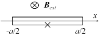
Figure B1: Long rectangular rf-SQUID. The “X” symbol denotes a Josephson junction (JJ).

To simplify the analysis, we introduce two functions $\psi\left(x,t\right),\xi\left(x,t\right)$ that are antisymmetric and symmetric respectively:

$$\phi\left(-x,t\right)-\phi\left(x,t\right)=\psi\left(x,t\right)$$ (18)

$$\phi\left(-x,t\right)+\phi\left(x,t\right)=\xi\left(x,t\right).$$ (19)

Since antisymmetric integrand disappears, we obtain

$$L_{TL}=L_{\psi}+L_{\xi}.$$ (20)

where

$$L_{\psi}=\frac{1}{2}\int_{0}^{a/2}dx\left\{\frac{c}{2}\left(\partial_{t}\psi\right)^{2}-\frac{1}{2l}\left(\partial_{x}\psi\right)^{2}\right\}$$ (21)

and

$$L_{\xi}=\frac{1}{2}\int_{0}^{a/2}dx\left\{\frac{c}{2}\left(\partial_{t}\xi\right)^{2}-\frac{1}{2l}\left(\partial_{x}\xi\right)^{2}\right\}.$$ (22)

Hence, the problem is divided into two non-interacting parts.

Consider the part involving $\xi\left(x,t\right)$ first. The Euler-Lagrange equation of motion is the wave equation. The first boundary condition $\xi\left(a/2,t\right)=0$ comes directly from the definition Eq. (14). On the other hand, we obtain $\partial_{x}\xi\left(x,t\right)=l\left\{i\left(x,t\right)-i\left(-x,t\right)\right\}$, which is linear in $x$ for small $x$ because only antisymmetric part of $i\left(x,t\right)$ contributes to $\partial_{x}\xi\left(x,t\right)$. Hence the second boundary condition is $\left[\partial_{x}\xi\left(x,t\right)\right]_{x=0}=0$. The harmonic form of solutions satisfying these boundary conditions is $\xi\left(x,t\right)\propto\cos\left(n\pi x/a\right)$ for $n=1,3,5,\cdots$. Quantization of the field $\xi\left(x,t\right)$ results in photons of various quantized energies, of which the lowest is $\pi\hbar/\left(a\sqrt{lc}\right)$. The field is free and it does not couple to the JJ under ideal conditions.

Next, we consider the field $\psi\left(x,t\right)$. Note that $\Phi\left(t\right)=\lim_{\varepsilon\rightarrow+0}\psi\left(\varepsilon,t\right)$. A boundary condition $\psi\left(a/2,t\right)=0$ follows from Eq. (14). The Lagrangian governing this part of the system is given by $L_{\psi}+L_{JJ}$. To simplify the analysis, we introduce another field $\hat{\psi}\left(x,t\right)=\psi\left(x,t\right)-\left(1-2x/a\right)\Phi\left(t\right)$, whose boundary condition is designed to be $\hat{\psi}\left(0,t\right)=\hat{\psi}\left(a/2,t\right)=0$. In terms of $\hat{\psi}\left(x,t\right)$ and $\Phi\left(t\right)$, the Lagrangian $L_{\psi}$ is

$$L_{\psi}=\frac{1}{2}\int_{0}^{a/2}dx\left\{\frac{c}{2}\left(\partial_{t}\hat{\psi}\right)^{2}-\frac{1}{2l}\left(\partial_{x}\hat{\psi}\right)^{2}\right\}+\frac{ca}{24}\dot{\Phi}^{2}-\frac{\Phi^{2}}{2la}$$

$$+\frac{c\dot{\Phi}}{2}\int_{0}^{a/2}dx\left(1-\frac{2x}{a}\right)\left(\partial_{t}\hat{\psi}\right),$$ (23)

where we used $\int_{0}^{a/2}dx\left(\partial_{x}\hat{\psi}\right)=\left[\hat{\psi}\right]_{x=0}^{x=a/2}=0$. Combining with $L_{JJ}$, we obtain

$$L_{\psi}+L_{JJ}=\frac{C}{2}\dot{\Phi}^{2}-E_{J}\cos\left(\frac{2\pi\Phi\left(t\right)}{\phi_{0}}\right)-\frac{\Phi^{2}}{2L}$$

$$+\frac{1}{2}\int_{0}^{a/2}dx\mathcal{L},$$ (24)

where we introduced parameters

$$C=C_{J}+ca/12$$ (25)

and $L=la$; and the Lagrangian density $\mathcal{L}$ of the continuous part of the system is

$$\mathcal{L}=\frac{c}{2}\left(\partial_{t}\hat{\psi}\right)^{2}-\frac{1}{2l}\left(\partial_{x}\hat{\psi}\right)^{2}+c\dot{\Phi}\left(1-\frac{2x}{a}\right)\left(\partial_{t}\hat{\psi}\right).$$ (26)

The Lagrangian $L_{\psi}+L_{JJ}$ consists of that of a lumped-circuit rf-SQUID, a free scalar field, and a velocity-dependent coupling between these. Note that the factor $12$ in Eq. (25) is a consequence of our particular choice of $\hat{\psi}\left(x,t\right)$, although the choice does simplify the form of the Lagrangian (24).

Full analysis of the system described in Eq. (24) would be complex and is beyond the scope of the present work. However, few preliminary remarks are in order. Pretend for the moment that the coupling term $c\dot{\Phi}\left(1-\frac{2x}{a}\right)\left(\partial_{t}\hat{\psi}\right)$ is absent. The field $\hat{\psi}$ has the harmonic form of solutions $\hat{\psi}\propto\sin\left(2n\pi x/a\right)$, where $n$ is a positive integer. This means that the minimum excitation energy of a photon is

$$\frac{2\pi\hbar}{a\sqrt{lc}}=\frac{4.1\>\mathrm{meV}}{\sqrt{\left(la/\mathrm{nH}\right)\left(ca/\mathrm{fF}\right)}}.$$ (27)

Hence in a typical parameter range, especially when the length $a$ of the rf-SQUID is not too large, the photon energy is higher than the qubit energy scale $\Delta$. This makes it likely that the photon degrees of freedom stay in the vacuum state adiabatically during the slow motion of the JJ degrees of freedom, not unlike cases in which the Born-Oppenheimer approximation is valid. A related phenomenon has been reported in the context of macroscopic quantum tunneling MQT latency (32).

The capacitance per unit length between the upper and the lower line of the circuit may be estimated by using the formula for two parallel thin rods

$$c=\frac{\pi\varepsilon_{eff}}{\ln\left(d/a\right)},$$ (28)

where $\varepsilon_{eff}$ is the effective electric permittivity, $d\cong 10\mu\mathrm{m}$ is the distance between the rods, and $a$ is the radius of the rods that should satisfy $a\ll d$. If the qubit is fabricated on a silicon wafer (possibly with a thin $\mathrm{Si}\mathrm{O}_{2}$ layer) then we obtain $\varepsilon_{eff}\cong\left(\varepsilon_{0}+\varepsilon_{\mathrm{Si}}\right)/2=6.34\varepsilon_{0}$. Ignoring the logarithmic factor, we obtain $c/12\cong{14.7\>\mathrm{fF}/\mathrm{mm}}$. Note that the factor $12$ appeared in Eq. (25).

Next, we consider a more favorable scenario. The value of $\varepsilon_{eff}$ could be significantly lowered by etching the Si wafer between the lines, possibly by deep reactive ion etching (DRIE) with the depth comparable to, or more than, $d$. (This could be beneficial also from the perspective of charged particle optical coherence. At least at the room temperature, decoherence of electron waves is observed when the electrons travel the distance of ${10\>\mathrm{mm}}$ along a semiconducting surface, while keeping the distance of several $\mu\mathrm{m}$ from the surface Hasselbach (30).) Furthermore, one could make an effort to make the factor $\ln\left(d/a\right)$ comparable to $\pi$. Provided that these measures can be made, then the capacitance per unit length is given simply as $c^{\prime}\cong\varepsilon_{0}$. We obtain $c^{\prime}/12\cong{0.74\>\mathrm{fF}/\mathrm{mm}}$ in this case.

Appendix C POTENTIAL ENERGY OF A SET OF WEAKLY-COUPLED RF-SQUIDS

We first make a minor digression and exhibit somewhat elementary results about a system of inductors. This is for the convenience of the reader, and also for showing approximations that we use. Let $A$ be a square matrix and $\boldsymbol{b},\boldsymbol{c}$ be vectors. It is straightforward to verify that

$$\left[\begin{array}[]{cc}A&\boldsymbol{b}\\ \boldsymbol{c}^{T}&d\end{array}\right]^{-1}=\left[\begin{array}[]{cc}A^{-1}+\Delta^{-1}A^{-1}\boldsymbol{b}\boldsymbol{c}^{T}A^{-1}&-\Delta^{-1}A^{-1}\boldsymbol{b}\\ -\Delta^{-1}\boldsymbol{c}^{T}A^{-1}&\Delta^{-1}\end{array}\right],$$ (29)

where the Schur complement is given as $\Delta=d-\boldsymbol{c}^{T}A^{-1}\boldsymbol{b}$. Now consider a system of coupled “internal” inductors, with the inductance matrix $l$ and the associated current vector $\boldsymbol{i}$ and the magnetic flux vector $\boldsymbol{\phi}$. This entire system is weakly coupled to a large “external” inductor $L$, with the current $I$ and the magnetic flux $\Phi$, that acts as a bias magnetic flux generator. The enlarged inductance matrix satisfies

$$\left[\begin{array}[]{c}\boldsymbol{\phi}\\ \Phi\end{array}\right]=\left[\begin{array}[]{cc}l&\boldsymbol{m}\\ \boldsymbol{m}^{T}&L\end{array}\right]\left[\begin{array}[]{c}\boldsymbol{i}\\ I\end{array}\right],$$ (30)

where values of mutual inductance are represented in the vector $\boldsymbol{m}$. The magnetic energy of the system is given as

$$U_{m}=\frac{1}{2}\left[\begin{array}[]{cc}\boldsymbol{i}^{T}&I\end{array}\right]\left[\begin{array}[]{cc}l&\boldsymbol{m}\\ \boldsymbol{m}^{T}&L\end{array}\right]\left[\begin{array}[]{c}\boldsymbol{i}\\ I\end{array}\right]=\frac{1}{2}\left[\begin{array}[]{cc}\boldsymbol{\phi}^{T}&\Phi\end{array}\right]\left[\begin{array}[]{cc}l&\boldsymbol{m}\\ \boldsymbol{m}^{T}&L\end{array}\right]^{-1}\left[\begin{array}[]{c}\boldsymbol{\phi}\\ \Phi\end{array}\right].$$ (31)

When applying the matrix inversion formula Eq. (29), we use the fact that the bias magnet is weakly coupled, and hence ignore the second and higher order terms with respect to the mutual inductance $\boldsymbol{m}$. Hence we obtain

$$U_{m}\cong\frac{1}{2}\left[\begin{array}[]{cc}\boldsymbol{\phi}^{T}&\Phi\end{array}\right]\left[\begin{array}[]{cc}l^{-1}&-l^{-1}\boldsymbol{m}/L\\ -\boldsymbol{m}^{T}l^{-1}/L&1/L\end{array}\right]\left[\begin{array}[]{c}\boldsymbol{\phi}\\ \Phi\end{array}\right]=\frac{1}{2}\boldsymbol{\phi}^{T}l^{-1}\boldsymbol{\phi}-\frac{\Phi}{L}\boldsymbol{m}^{T}l^{-1}\boldsymbol{\phi}+\frac{\Phi^{2}}{2L}.$$ (32)

Since we decided to ignore higher order terms in $\boldsymbol{m}$, this expression is further approximated as

$$U_{m}\cong\frac{1}{2}\left(\boldsymbol{\phi}-\frac{\Phi}{L}\boldsymbol{m}\right)^{T}l^{-1}\left(\boldsymbol{\phi}-\frac{\Phi}{L}\boldsymbol{m}\right)+\frac{\Phi^{2}}{2L},$$ (33)

where the second term will be neglected in the followings. (Such an omission may not always be justified. See Ref. Ralph et al (22).) Clearly, $\frac{\Phi}{L}\boldsymbol{m}\cong\boldsymbol{m}I$ represents the external bias flux and we regard $\boldsymbol{\phi}-\frac{\Phi}{L}\boldsymbol{m}$ as a set of magnetic flux generated by the current flowing in each internal inductor.

Returning to our system, a magnetic flux $\phi_{k}+\phi_{0}/2$ threads the $k-$th rf-SQUID. The first term $\phi_{k}$ is generated by the current in the $k-$th rf-SQUID ring, while the second term $\phi_{0}/2$ is the bias flux applied externally. We find (See Eq. (33)) the magnetic energy stored in the system, if we can invert the inductance matrix of the system of coupled rf-SQUIDs. The inductance matrix may be written in the form of $L\mathbf{A}$, where the square tridiagonal matrix $\mathbf{A}$ with elements $a_{i,k}$ has the diagonal entries $a_{i,i}=1$ and the adjacent off-diagonal entries $a_{i,i+1}=a_{i,i-1}=M/L$. In order to invert this, we make an assumption $M/L\ll 1$. To the first order in $\delta$, $\mathbf{B}=\mathbf{A}^{-1}$ has the diagonal entries $b_{i,i}=1$ and the off-diagonal entries $b_{i,i+1}=b_{i,i-1}=-M/L$, while all other entries are zero. Hence

$$U_{m}\cong\frac{1}{2L}\sum_{k=1}^{N}\phi_{k}^{2}-\frac{M}{L^{2}}\sum_{k=1}^{N-1}\phi_{k}\phi_{k+1}$$

$$\cong\frac{1}{2\left(L+2M\right)}\sum_{k=1}^{N}\phi_{k}^{2}+\frac{M}{2L^{2}}\sum_{k=1}^{N-1}\left(\phi_{k+1}-\phi_{k}\right)^{2},$$ (34)

to the first order in $M/L$. We may argue that the level of accuracy is maintained by this “approximation” anyway, because non-zero mutual inductance beyond the nearest neighbor rf-SQUIDs should exist in the first place.

The condition $M/L\ll 1$ is satisfied in the parameter region of interest. The rf-SQUID mentioned in the main text has device parameters $C={10.0\>\mathrm{fF}}$, ${L=800\>\mathrm{pH}}$ and $\beta=1.11$, for which $\Delta={1.1\times 10^{-23}\>\mathrm{J}}$. On the other hand, we expect to use the composite qubit in the region $R\cong 1$ near the QCP, which translates to $J=M\phi_{0}^{2}/2N^{2}L^{2}\cong\Delta/2$, or equivalently $M/L\cong LN^{2}\Delta/\phi_{0}^{2}$. The right hand side turns out to be $3.2\times 10^{-2}$, which justifies the use of the aforementioned condition $M/L\ll 1$. (This argument is not circular as one could have picked such $M/L$ first, then developed approximate expressions based on it, and later found that $R$ happens to be close to $1$.)

Appendix D RENORMALIZING THE TRANSVERSE-FIELD ISING MODEL WITH A SMALL LONGITUDINAL FIELD

We extend the renormalization analysis of the transverse-field Ising model with a zero longitudinal-field (i.e. $\varepsilon=0$), originally due to Fernandez-Pacheco Fernandez-Pacheco (28, 33), to the $\varepsilon\neq 0$ case. The straightforward but lengthy process of extension is presented below. Note that detailed studies on the transverse-field Ising system with a longitudinal field have appeared in the literature longitudinal field and trans-field Ising (34).

For block renormalization purposes, we rewrite the Hamiltonian (Eq. (2) in the main text)

$$H=-J\sum_{i}\sigma_{i}^{z}\sigma_{i+1}^{z}-h\sum_{i}\sigma_{i}^{x}-\varepsilon\sum_{i}\sigma_{i}^{z},$$ (35)

where the index $i$ points to each spin, as a sum of intra-block and inter-block terms

$$H=\sum_{j}H_{j}^{intra}+\sum_{j}H_{j}^{inter},$$ (36)

$$H_{j}^{intra}=-h\sigma_{2j-1}^{x}-\varepsilon\sigma_{2j-1}^{z}-J\sigma_{2j-1}^{z}\sigma_{2j}^{z},$$ (37)

$$H_{j}^{inter}=-h\sigma_{2j}^{x}-\varepsilon\sigma_{2j}^{z}-J\sigma_{2j-2}^{z}\sigma_{2j-1}^{z},$$ (38)

where $j$ points to each block of $2$ spins. Notations such as $\sigma_{i}^{z}$ imply identity operators for all spins except the spin $i$. We call spins with an odd index “slave spins” and the rest “master spins”. The Hilbert space pertaining to the $i$-th spin is spanned by $|s\rangle_{i}$, where $s=\pm 1$ denotes one of the eigenvalues of the operator $\sigma_{i}^{z}$. The identity operator pertaining to the $i$-th spin is denoted $I_{i}$.

We first focus on the intra-block Hamiltonian (37) and seek energy eigenstates of the form $\left(a|1\rangle_{2j-1}+b|-1\rangle_{2j-1}\right)\otimes|s\rangle_{2j}$. We find eigenvalues

$$\lambda_{\pm,s}=\pm\sqrt{h^{2}+\left(sJ+\varepsilon\right)^{2}},$$ (39)

and respectively corresponding eigenvectors $|\lambda_{\pm,s}\rangle_{2j-1}\otimes|s\rangle_{2j}$, where

$$|\lambda_{\pm,s}\rangle_{2j-1}=F\left\{-h|1\rangle_{2j-1}+\left[\left(sJ+\varepsilon\right)\pm\sqrt{h^{2}+\left(sJ+\varepsilon\right)^{2}}\right]|-1\rangle_{2j-1}\right\},$$ (40)

where $F$ is a real and positive normalization factor that depends on $s$ and $\lambda_{\pm}$. An equivalent expression is

$$|\lambda_{\pm,s}\rangle_{2j-1}=F\left\{\left[\left(sJ+\varepsilon\right)\mp\sqrt{h^{2}+\left(sJ+\varepsilon\right)^{2}}\right]|1\rangle_{2j-1}+h|-1\rangle_{2j-1}\right\},$$ (41)

which may be useful in the $h\rightarrow 0$ limit for some combinations of $s$ and $\lambda_{\pm}$.

We block-renormalize the system by demanding that each slave spin $2j-1$ is in the ground state $|\lambda_{-,s}\rangle_{2j-1}$of the associated intra-block Hamiltonian $H_{j}^{intra}$. To avoid cluttered presentation, we use $|g_{s}\rangle_{2j-1}\equiv|\lambda_{-,s}\rangle_{2j-1}$ and $g_{s}\equiv\lambda_{-,s}$ below. Note that the state $|g_{s}\rangle_{2j-1}$ depends on the state $|s\rangle_{2j}$ of the associated master spin $2j$. To be concrete, the renormalized Hamiltonian $H_{R}$ is defined as

$$H_{R}=P^{\dagger}HP,$$ (42)

where $P=\otimes_{j}P_{j}$ and

$$P_{j}=|g_{1}\rangle_{2j-1}\otimes\left(|1\rangle_{2j}\langle 1|_{2j}\right)+|g_{-1}\rangle_{2j-1}\otimes\left(|-1\rangle_{2j}\langle-1|_{2j}\right),$$ (43)

although one might prefer to use states of $j$-th renormalized spin $\langle\pm 1_{R}|_{j}$ instead of $\langle\pm 1|_{2j}$.

We use the following relations to obtain $H_{R}$.

$$P_{j}^{\dagger}H_{j}^{intra}P_{j}=g_{1}|1\rangle_{2j}\langle 1|_{2j}+g_{-1}|-1\rangle_{2j}\langle-1|_{2j},$$ (44)

$$P_{j}^{\dagger}\sigma_{2j}^{z}P_{j}=P_{j}^{\dagger}\left(|1\rangle_{2j}\langle 1|_{2j}-|-1\rangle_{2j}\langle-1|_{2j}\right)P_{j}=|1\rangle_{2j}\langle 1|_{2j}-|-1\rangle_{2j}\langle-1|_{2j}=\sigma_{2j}^{z},$$ (45)

$$P_{j}^{\dagger}\sigma_{2j}^{x}P_{j}=\langle g_{-1}|g_{1}\rangle_{2j-1}|-1\rangle_{2j}\langle 1|_{2j}+\langle g_{1}|g_{-1}\rangle_{2j-1}|1\rangle_{2j}\langle-1|_{2j}=\alpha\sigma_{2j}^{x},$$ (46)

where

$$\alpha=\langle g_{-1}|g_{1}\rangle_{2j-1}=\langle g_{1}|g_{-1}\rangle_{2j-1}$$ (47)

and

$$P_{j}^{\dagger}P_{j-1}^{\dagger}\sigma_{2j-2}^{z}\sigma_{2j-1}^{z}P_{j-1}P_{j}$$

$$=\left(P_{j-1}^{\dagger}\sigma_{2j-2}^{z}P_{j-1}\right)\left(P_{j}^{\dagger}\sigma_{2j-1}^{z}P_{j}\right),$$ (48)

$$P_{j}^{\dagger}\sigma_{2j-1}^{z}P_{j}=\beta_{1}|1\rangle_{2j}\langle 1|_{2j}+\beta_{-1}|-1\rangle_{2j}\langle-1|_{2j},$$ (49)

where

$$\beta_{1}=\langle g_{1}|\sigma_{2j-1}^{z}|g_{1}\rangle_{2j-1},\>\beta_{-1}=\langle g_{-1}|\sigma_{2j-1}^{z}|g_{-1}\rangle_{2j-1}.$$ (50)

To proceed further, we assume $\varepsilon\ll h,J$ and retain only the first order terms in $\varepsilon$ in the following expressions. We obtain

$$g_{\pm 1}=-\sqrt{h^{2}+J^{2}}\left(1\pm\frac{J\varepsilon}{h^{2}+J^{2}}\right),$$ (51)

$$|g_{1}\rangle=F_{1}\left\{-h|1\rangle_{2j-1}+\left[J-\sqrt{h^{2}+J^{2}}+\varepsilon\left(1-\frac{J}{\sqrt{h^{2}+J^{2}}}\right)\right]|-1\rangle_{2j-1}\right\},$$ (52)

$$|g_{-1}\rangle=F_{-1}\left\{-h|1\rangle_{2j-1}-\left[J+\sqrt{h^{2}+J^{2}}-\varepsilon\left(1+\frac{J}{\sqrt{h^{2}+J^{2}}}\right)\right]|-1\rangle_{2j-1}\right\},$$ (53)

where

$$F_{\pm 1}=\frac{1}{\sqrt{h^{2}+\left(J\mp\sqrt{h^{2}+J^{2}}\right)^{2}}}\left\{1+\frac{\varepsilon}{\sqrt{h^{2}+J^{2}}}\frac{\left(J\mp\sqrt{h^{2}+J^{2}}\right)^{2}}{h^{2}+\left(J\mp\sqrt{h^{2}+J^{2}}\right)^{2}}\right\},$$ (54)

and

$$F_{1}F_{-1}=\frac{1}{2h\sqrt{h^{2}+J^{2}}}\left(1+\frac{\varepsilon}{\sqrt{h^{2}+J^{2}}}\right).$$ (55)

We further obtain

$$\alpha=F_{1}F_{-1}2h^{2}\left(1-\frac{\varepsilon}{\sqrt{h^{2}+J^{2}}}\right)=\frac{h}{\sqrt{h^{2}+J^{2}}}.$$ (56)

This is a property along the $x$ axis, which should not be affected by the parameter $\varepsilon$ linearly, because nonzero $\varepsilon$ breaks symmetry with respect to the $z$ axis. Continuing, using an identity

$$\frac{J^{2}\pm J\sqrt{h^{2}+J^{2}}}{h^{2}+J^{2}\pm J\sqrt{h^{2}+J^{2}}}=\pm\frac{J}{\sqrt{h^{2}+J^{2}}},$$ (57)

we obtain

$$\beta_{\pm 1}=F_{\pm 1}^{2}\left\{h^{2}-\left(J\mp\sqrt{h^{2}+J^{2}}\right)^{2}+\frac{2\varepsilon\left(J\mp\sqrt{h^{2}+J^{2}}\right)^{2}}{\sqrt{h^{2}+J^{2}}}\right\}$$

$$=\pm\frac{J}{\sqrt{h^{2}+J^{2}}}\left\{1+\frac{2\varepsilon}{\sqrt{h^{2}+J^{2}}}\frac{2h^{2}\left(J\mp\sqrt{h^{2}+J^{2}}\right)^{2}}{h^{4}-\left(J\mp\sqrt{h^{2}+J^{2}}\right)^{4}}\right\}$$

$$=\pm\frac{J}{\sqrt{h^{2}+J^{2}}}\left\{1\pm\frac{\varepsilon h^{2}}{J\left(h^{2}+J^{2}\right)}\right\}.$$ (58)

Combining these results, we obtain

$$P_{j}^{\dagger}H_{j}^{intra}P_{j}=-\sqrt{h^{2}+J^{2}}I_{2j}-\frac{J\varepsilon}{\sqrt{h^{2}+J^{2}}}\sigma_{2j}^{z},$$ (59)

where the first term is an unimportant additive constant and we will omit it below. We further get

$$P_{j}^{\dagger}\sigma_{2j-1}^{z}P_{j}=\frac{\varepsilon h^{2}}{\left(h^{2}+J^{2}\right)^{3/2}}I_{2j}+\frac{J}{\sqrt{h^{2}+J^{2}}}\sigma_{2j}^{z}$$ (60)

and hence

$$P_{j}^{\dagger}P_{j-1}^{\dagger}H_{j}^{inter}P_{j-1}P_{j}=-P_{j}^{\dagger}P_{j-1}^{\dagger}\left(h\sigma_{2j}^{x}+\varepsilon\sigma_{2j}^{z}+J\sigma_{2j-2}^{z}\sigma_{2j-1}^{z}\right)P_{j-1}P_{j}$$

$$=-\left(\frac{h^{2}}{\sqrt{h^{2}+J^{2}}}\sigma_{2j}^{x}+\varepsilon\sigma_{2j}^{z}+\frac{J^{2}}{\sqrt{h^{2}+J^{2}}}\sigma_{2j-2}^{z}\sigma_{2j}^{z}+\frac{\varepsilon Jh^{2}}{\left(h^{2}+J^{2}\right)^{3/2}}\sigma_{2j-2}^{z}\right).$$ (61)

Thus, the renormalized Hamiltonian has the same form as the original one:

$$H_{R}=-J_{R}\sum_{j}\sigma_{2j}^{z}\sigma_{2j+2}^{z}-h_{R}\sum_{j}\sigma_{2j}^{x}-\varepsilon_{R}\sum_{j}\sigma_{2j}^{z},$$ (62)

where renormalized parameters are

$$J_{R}=\frac{J^{2}}{\sqrt{h^{2}+J^{2}}},$$ (63)

$$h_{R}=\frac{h^{2}}{\sqrt{h^{2}+J^{2}}},$$ (64)

$$\varepsilon_{R}=\varepsilon\left\{1+\frac{J}{\sqrt{h^{2}+J^{2}}}\left(1+\frac{h^{2}}{h^{2}+J^{2}}\right)\right\}.$$ (65)

Appendix E EXPECTED ERRORS IN ENTANGLEMENT-ENHANCED ELECTRON MICROSCOPY: A PRELIMINARY ANALYSIS

In EEEM, the composite qubit ideally holds magnetic flux of either zero or $\phi_{0}$. As mentioned in the main text, the magnetic flux difference between the two qubit states may be slightly different from the ideal $\phi_{0}$. This is the first kind of error, which could be nullified by adjusting $\beta$ of each constituent qubit. However, we should like to see how sensitive the system is to such an error. The second kind of nonideality is that the magnetic flux held by the composite qubit may not be quantum mechanically well-defined. Below we study these two kinds of errors in turn. However, the problem is complex and our study presented here is preliminary.

To evaluate the first kind of error, we assume that the qubit holds magnetic flux of either $\left(1-P\right)\phi_{0}/2$ or $\left(1+P\right)\phi_{0}/2$, where the real parameter $P$ is close to, but smaller than, the ideal value $1$. Note that the difference is $P\phi_{0}$. We adjusted their mean to be $\phi_{0}/2$ for later convenience. This adjustment corresponds to shifting of the phase of the electron waves going through the magnetic flux ring, which most likely means simply a shift of the focus of the objective lens in practice. Let $\zeta$ be $\left(\pi/4\right)\left(1-P\right)$, which is small. Following the EEEM literature, the two qubit states with flux $\left(1-P\right)\phi_{0}/2$ and $\left(1+P\right)\phi_{0}/2$ are respectively denoted by $|0\rangle$ and $|1\rangle$, although these are denoted by $\mid\Uparrow^{\prime}\rangle$ and $\mid\Downarrow^{\prime}\rangle$ in the main text. Due to the AB effect, with the qubit state $|1\rangle$ the electron passing through the magnetic flux ring (the electron state $|a\rangle_{e}=\left(|0\rangle_{e}-|1\rangle_{e}\right)\sqrt{2}$) receives a phase factor $-e^{-i\zeta}$ whereas the electron passing by the ring (the electron state $|s\rangle_{e}=\left(|0\rangle_{e}+|1\rangle_{e}\right)\sqrt{2}$) receives a phase factor $e^{i\zeta}$. To make analysis simpler, we assume that a small amount of vector potential $\boldsymbol{A}$ (in the Coulomb gauge. See arguments in Ref. q-interface (6)) remains $outside$ the magnetic flux ring generated by the qubit, in the following way: When the qubit state is $|0\rangle$, then the electron states $|a\rangle_{e}$ and $|s\rangle_{e}$ receives phase factors $e^{i\zeta}$ and $e^{-i\zeta}$, respectively. Put differently, the difference in the phase shifts, for electrons in the states $|a\rangle_{e}$ and $|s\rangle_{e}$, is less than the ideal $\pi$ in the case of the qubit state $|1\rangle$, but the mean phase shift is assumed to be $\pi/2$; whereas the phase shift difference is more than the ideal $0$ when the qubit is in the state $|0\rangle$ but the mean phase shift is assumed to be $0$. The following formulae should be modified if this simplifying assumption is not used.

The initial states for the electron and the qubit are respectively $|0\rangle_{e}$ and $|s\rangle=\left(|0\rangle+|1\rangle\right)/\sqrt{2}$. After interaction, the state of the composite system becomes

$$\cos\zeta\frac{|00\rangle+|11\rangle}{\sqrt{2}}+i\sin\zeta\frac{|01\rangle-|10\rangle}{\sqrt{2}}$$

$$\cong\frac{|00\rangle+|11\rangle}{\sqrt{2}}+i\zeta\frac{|01\rangle-|10\rangle}{\sqrt{2}},$$ (66)

where $|00\rangle=|0\rangle_{e}\otimes|0\rangle$ etc. Then the electron wave goes through the specimen and the state $|0\rangle_{e}$ receives a phase factor $e^{2is}$ relative to the state $|1\rangle_{e}$. Hence we have

$$\frac{e^{is}|00\rangle+e^{-is}|11\rangle}{\sqrt{2}}+i\zeta\frac{e^{is}|01\rangle-e^{-is}|10\rangle}{\sqrt{2}}.$$ (67)

For simplicity, we assume that the electron is detected either in the state $|s\rangle_{e}$ or $|a\rangle_{e}$; or in other words $\left(|0\rangle_{e}\pm|1\rangle_{e}\right)/\sqrt{2}$. The qubit is left in respective states

$$\frac{e^{is}|0\rangle\pm e^{-is}|1\rangle}{\sqrt{2}}+i\zeta\frac{e^{is}|1\rangle\mp e^{-is}|0\rangle}{\sqrt{2}}$$

$$=\frac{1}{\sqrt{2}}\left\{\left(e^{is}\mp i\zeta e^{-is}\right)|0\rangle\pm\left(e^{-is}\pm i\zeta e^{is}\right)|1\rangle\right\}.$$ (68)

The effect of non-zero $\zeta$ must be corrected unless $\zeta\ll s$. Since $s$ is not known a priori, one may need to employ approximations such as $i\zeta e^{-is}\cong i\zeta$ on grounds that both the parameters $\zeta$ and $s$ are small. Further study is needed to determine the region of validity of such approximations. Note that, in high resolution cryoelectron microscopy of biological specimens, we deal with values of $s$ as small as $0.01$ adaptive EM (35). Further note that factors such as $\left(e^{-is}\pm i\zeta e^{is}\right)$ are multiplied a few tens of times in EEEM before the qubit is measured, although we only discussed the case of single factors for the sake of simplicity.

We turn to the second issue of the qubit states that do not have definite magnetic flux values, but have quantum mechanically smeared values. We would need to analyze the composite qubit not far from the QCP to obtain the details of such states for a detailed study. Instead, in order to see the general structure of the problem, here we schematically write the state corresponding to Eq. (68) as

$$\left\{c\left(e^{is}\mp i\zeta e^{-is}\right)|0\rangle+c^{\prime}\left(e^{is}\mp i\zeta^{\prime}e^{-is}\right)|0^{\prime}\rangle+\cdots\right\}$$

$$\pm\left\{d\left(e^{-is}\pm i\zeta e^{is}\right)|1\rangle+d^{\prime}\left(e^{-is}\pm i\zeta^{\prime}e^{is}\right)|1^{\prime}\rangle+\cdots\right\},$$ (69)

where the primes indicate entities with slightly different magnetic flux values with respect to the entities without the primes; and $c,d$ are quantum amplitudes. On the other hand, if the qubit’s basis states are written as

$$|\mathbf{0}\rangle=c|0\rangle+c^{\prime}|0^{\prime}\rangle+\cdots,\>|\mathbf{1}\rangle=d|1\rangle+d^{\prime}|1^{\prime}\rangle+\cdots,$$ (70)

then the state in Eq. (69) is written as, up to a normalization factor

$$e^{is+\zeta_{0}}|\mathbf{0}\rangle+e^{-is+\zeta_{1}}|\mathbf{1}\rangle+\sum|\textrm{excited states}\rangle.$$ (71)

Further study is required to find the phase shifts $\zeta_{0},\zeta_{1}$ that must be corrected, as well as the probability of the qubit to get excited, which causes an error that is unlikely to be correctable. Note that values of $\zeta_{0},\zeta_{1}$ depend on the outcomes of electron detection events and also weakly on the unknown parameter $s$.

Appendix F EVOLUTION OF HAMILTONIAN PARAMETERS UPON RENORMALIZATION

The Hamiltonian parameters $h$ and $\varepsilon$ change to renormalized values $h^{\prime\prime}$ and $\varepsilon^{\prime\prime}$ after $2$ iterations of block renormalization. Figure F1 shows ratios $h^{\prime\prime}/h$ and $\varepsilon^{\prime\prime}/\varepsilon$ plotted against the parameter $R$ of the original system. The plotted functions are

$$\frac{h^{\prime\prime}}{h}=\frac{R}{\sqrt{1+R^{2}}}\cdot\frac{R^{2}}{\sqrt{1+R^{4}}},$$ (72)

and

$$\frac{\varepsilon^{\prime\prime}}{\varepsilon}=\left(1+\frac{1+2R^{2}}{\left(1+R^{2}\right)^{3/2}}\right)\left(1+\frac{1+2R^{4}}{\left(1+R^{4}\right)^{3/2}}\right).$$ (73)

The final renormalized spin corresponds to $N=2^{2}=4$ spins in the original system.

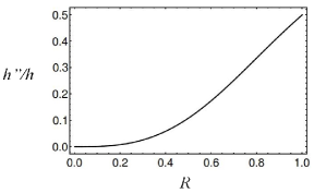
(a)

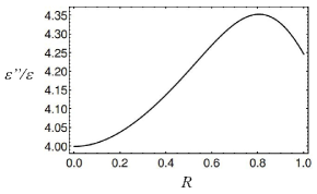
(b)

Figure F1: Changes of the parameters $h$ and $\varepsilon$ after $2$ iterations of block renormalization.

References

- (1) H. Okamoto, T. Latychevskaia, and H.-W. Fink, Appl. Phys. Lett. , 164103 (2006).
- (2) W. P. Putnam and M. F. Yanik, Phys. Rev. A , 040902(R) (2009).
- (3) P. Kruit, R. G. Hobbs, C.-S. Kim, Y. Yang, V. R. Manfrinato, J. Hammer, S. Thomas, P. Weber, B. Klopfer, C. Kohstall, T. Juffmann, M. A. Kasevich, P. Hommelhoff, and K. K. Berggren, Ultramicroscopy , 31 (2016).
- (4) H. Okamoto, Phys. Rev. A , 043810 (2012).
- (5) H. Okamoto and Y. Nagatani, Appl. Phys. Lett. , 062604 (2014).
- (6) H. Okamoto, Phys. Rev. A , 053805 (2015).
- (7) A. Widom, J. Low Temp. Phys. , 449 (1979); A. J. Leggett, Prog. Theor. Phys. Suppl. , 80 (1980); J. Clarke, A. N. Cleland, M. H. Devoret, D. Eeteve, J. M. Martinis, Science , 992 (1988).
- (8) For an alternative scheme aiming at approaching the Heisenberg limit, see T. Juffmann, S. A. Koppell, B. B. Klopfer, C. Ophus, R. M. Glaeser, M. A. Kasevich, Sci. Rep. , 1699 (2017). See also H. Okamoto, Phys. Rev. A , 043807 (2010).
- (9) W. Ehrenberg and R. E. Siday, Proc. Phys. Soc. Ser. B , 8 (1949); Y. Aharonov and D. Bohm, Phys. Rev. , 485 (1959).
- (10) A. Tonomura, A. Osakabe, T. Matsuda, T. Kawasaki, J. Endo, S. Yano, and H. Yamada, Phys. Rev. Lett. , 792 (1986).
- (11) J. R. Friedman, V. Patel, W. Chen, S. K. Tolpygo, and J. E. Lukens, Nature (London) , 43 (2000); R. Harris, M. W. Johnson, S. Han, A. J. Berkley, J. Johansson, P. Bunyk, E. Ladizinsky, S. Govorkov, M. C. Thom, S. Uchaikin, B. Bumble, A. Fung, A. Kaul, A. Kleinsasser, M. H. S. Amin, and D. V. Averin, Phys. Rev. Lett. , 117003 (2008). For early experiments, see e.g. W. den Boer and R. de Bruyn Ouboter, Physica , 185 (1980); R. J. Prance, A. P. Long, T. D. Clark, A. Widom, J. E. Mutton, J. Sacco, M. W. Potts, G. Megaloudis, and F. Goodall, Nature , 543 (1981).
- (12) A. Kovacs, Z.-A. Li, K. Shibata, R. E. Dunin-Borkowski, Resolution and Discovery , 2 (2016).
- (13) S. J. Weber, G. O. Samach, D. Hover, S. Gustavsson, D. K. Kim, A. Melville, D. Rosenberg, A. P. Sears, F. Yan, J. L. Yoder, W. D. Oliver, and A. J. Kerman, Phys. Rev. Applied , 014004 (2017).
- (14) R. Harris, F. Brito, A. J. Berkley, J. Johansson, M. W. Johnson, T. Lanting, P. Bunyk, E. Ladizinsky, B. Bumble, A. Fung, A. Kaul, A. Kleinsasser and S. Han, New J. Phys. , 123022 (2009).
- (15) R. Harris, M. W. Johnson, S. Han, A. J. Berkley, J. Johansson, P. Bunyk, E. Ladizinsky, S. Govorkov, M. C. Thom, S. Uchaikin, B. Bumble, A. Fung, A. Kaul, A. Kleinsasser, M. H. S. Amin and D. V. Averin, Phys. Rev. Lett. , 117003 (2008); T. Lanting, A. J. Berkley, B. Bumble, P. Bunyk, A. Fung, J. Johansson, A. Kaul, A. Kleinsasser, E. Ladizinsky, F. Maibaum, R. Harris, M. W. Johnson, E. Tolkacheva and M. H. S. Amin, Phys. Rev. B , 060509 (2009); T. Lanting, M. H. S. Amin, M. W. Johnson, F. Altomare, A. J. Berkley, S. Gildert, R. Harris, J. Johansson, P. Bunyk, E. Ladizinsky, E. Tolkacheva and D. V. Averin, Phys. Rev. B , 180502(R) (2011).
- (16) The parameter in the MRT studies MRT noise measurements (15) is noise in terms of energy and should give the rough magnitude of magnetic flux noise.
- (17) M. Schmelz, V. Zakosarenko, A. Chwala, T. Sch nau, R. Stolz, S. Anders, S. Linzen and H. G. Meyer, IEEE Trans. Appl. Supercond. , 1600804 1-5 (2016).
- (18) S. Han, J. Lapointe, and J. E. Lukens, Phys. Rev. Lett. , 1712 (1989); S. Han, J. Lapointe, and J. E. Lukens, Phys. Rev. Lett. , 810 (1991).
- (19) R. Harris, J. Johansson, A. J. Berkley, M. W. Johnson, T. Lanting, S. Han, P. Bunyk, E. Ladizinsky, T. Oh, I. Perminov, E. Tolkacheva, S. Uchaikin, E. Chapple, C. Enderud, C. Rich, M. Thom, J. Wang, B. Wilson and G. Rose, Phys. Rev. B , 134510 (2010).
- (20) A. Maassen van den Brink, A. J. Berkley, and M. Yalowsky, New J. Phys. , 230 (2005); J. B. Majer, F. G. Paauw, A. C. J. ter Haar, C. J. P. M. Harmans, and J. E. Mooij, Phys. Rev. Lett. , 090501 (2005); S. H. W. van der Ploeg, A. Izmalkov, A. Maassen van den Brink, U. Huebner, M. Grajcar, E. Il’ichev, H.-G. Meyer, and A. M. Zagoskin, Phys. Rev. Lett. , 057004 (2007); R. Harris, A. J. Berkley, M. W. Johnson, P. Bunyk, S. Govorkov, M. C. Thom, S. Uchaikin, A. B. Wilson, J. Chung, E. Holtham, J. D. Biamonte, A. Yu. Smirnov, M. H. S. Amin, and A. Maassen van den Brink, Phys. Rev. Lett. , 177001 (2007); R. Harris, T. Lanting, A. J. Berkley, J. Johansson, M. W. Johnson, P. Bunyk, E. Ladizinsky, N. Ladizinsky, T. Oh, and S. Han, Phys. Rev. B , 052506 (2009).
- (21) M. G. Castellano, F. Chiarello, G. Torrioli, and P. Carelli, Supercond. Sci. Technol. , 1158 (2006).
- (22) J. F. Ralph, T. D. Clark, M. J. Everitt, and P. Stiffell, Phys. Rev. B , 180504(R) (2001).
- (23) M. G. Castellano, F. Chiarello, R. Leoni, F. Mattioli, G. Torrioli, P. Carelli, M. Cirillo, C. Cosmelli, A. de Waard, G. Frossati, N. Gronbech-Jensen, and S. Poletto, Phys. Rev. Lett. , 177002 (2007).
- (24) A free version of InductEX is available at: “http://www0.sun.ac.za/ix/”. Also see: C. J. Fourie, IEEE Trans. Appl. Supercond., , 1300209 (2015); InductEX in turn is based on FastHenry described in: M. Kamon, M. J. Tsuk, and J. White, IEEE Trans. Microw. Theory Techn., , 1750 (1994). The calculation performed here was sensitive to the exact shape of the loop. We assumed wide and thick aluminum lines. The lengths of the lines were , , and to verify the linear dependence. We used two London penetration depth of and , which resulted in variation of the value of inductance per unit length. For the London penetration depth of aluminum, see: K. Steinberg, M. Scheffler, and M. Dressel, Phys. Rev. B , 214517 (2008).
- (25) S. Sachdev, Quantum Phase Transitions (Cambridge University Press, Cambridge UK, 1999).
- (26) M. W. Johnson, M. H. S. Amin, S. Gildert, T. Lanting, F. Hamze, N. Dickson, R. Harris, A. J. Berkley, J. Johansson, P. Bunyk, E. M. Chapple, C. Enderud, J. P. Hilton, K. Karimi, E. Ladizinsky, N. Ladizinsky, T. Oh, I. Perminov, C. Rich, M. C. Thom, E. Tolkacheva, C. J. S. Truncik, S. Uchaikin, J. Wang, B. Wilson, and G. Rose, Nature , 194 (2011).
- (27) T. Lanting, A. J. Przybysz, A. Yu. Smirnov, F. M. Spedalieri, M. H. S. Amin, A. J. Berkley, R. Harris, F. Altomare, S. Boixo, P. Bunyk, N. Dickson, C. Enderud, J. P. Hilton, E. Hoskinson, M. W. Johnson, E. Ladizinsky, N. Ladizinsky, R. Neufeld, T. Oh, I. Perminov, C. Rich, M. C. Thom, E. Tolkacheva, S. Uchaikin, A. B. Wilson and G. Rose, Phys. Rev. X , 021041 (2014).
- (28) A. Fernandez-Pacheco, Phys. Rev. D , 3173 (1979).
- (29) M. G. Castellano, F. Chiarello, P. Carelli, C. Cosmelli, F. Mattioli, and G. Torrioli, New J. Phys. , 043047 (2010).
- (30) P. Sonnentag and F. Hasselbach, Phys. Rev. Lett. , 200402 (2007).
- (31) R. J. Schoelkopf, A. A. Clerk, S. M. Girvin, K. W. Lehnert and M. H. Devoret, in Y. V. Nazarov (eds), Qubits as Spectrometers of Quantum Noise, in Quantum Noise in Mesoscopic Physics, NATO Science Series II, Springer, Dordrecht, 2003, vol. 97, p. 175.
- (32) C. Urbina, D. Esteve, J. M. Martinis, E. Turlota, M. H. Devoret, H. Grabert, and S. Linkwitzb, Measurement of the latency time of Macroscopic Quantum Tunneling, Physica B , 26-31 (1991).
- (33) See also C. Monthus, J. Stat. Mech. P01023 (2015).
- (34) See e.g. K. Uzelac, R. Jullien, and P. Pfeuty, Phys. Rev. B , 436 (1980).
- (35) H. Okamoto, Phys. Rev. A , 043807 (2010).