Understanding solar torsional oscillations from global dynamo models

Abstract

The phenomenon of solar “torsional oscillations” (TO) represents migratory zonal flows associated with the solar cycle. These flows are observed on the solar surface and, according to helioseismology, extend through the convection zone. We study the origin of the TO using results from a global MHD simulation of the solar interior that reproduces several of the observed characteristics of the mean-flows and magnetic fields. Our results indicate that the magnetic tension (MT) in the tachocline region is a key factor for the periodic changes in the angular momentum transport that causes the TO. The torque induced by the MT at the base of the convection zone is positive at the poles and negative at the equator. A rising MT torque at higher latitudes causes the poles to speed-up, whereas a declining negative MT torque at the lower latitudes causes the equator to slow-down. These changes in the zonal flows propagate through the convection zone up to the surface. Additionally, our results suggest that it is the magnetic field at the tachocline that modulates the amplitude of the surface meridional flow rather than the opposite as assumed by flux-transport dynamo models of the solar cycle.

1 Introduction

The Sun exhibits a periodic variation of its angular velocity that is about $\pm 0.5$% of the average rotation profile. These so-called torsional oscillations (TO) represent acceleration and deceleration of the zonal component of the plasma flow during the solar cycle (Howard & Labonte 1980; Kosovichev & Schou 1997; Toomre et al. 2000; Howe et al. 2000; Antia & Basu 2001; Howe et al. 2005; Vorontsov et al. 2002). Two branches of the oscillations have been observed. The first branch, migrating from  40^o latitude toward the equator, appears a few years prior to the start of a solar cycle and disappears by the end of the cycle. The second branch, at higher latitudes, migrates toward the polar regions. For the solar cycles 22 and 23, the amplitude of the polar branch was larger than that of the equatorial branch. For cycle 24, the polar branch is significantly weaker than it was in the previous cycles (Zhao et al. 2014; Komm et al. 2014; Kosovichev & Zhao 2016). Additionally, recent helioseismology observations showed that the TO correlate with the variations of the meridional flows (Zhao et al. 2014; Komm et al. 2015). The evident dependence of the TO on the solar activity cycle provides a unique opportunity to explore the interaction between large-scale magnetic field and flows. Furthermore, understanding the nature of TO could provide a way to infer the distribution of magnetic fields below the solar photosphere.

The origin of the TO is still unclear. It is puzzling that the equatorward branch starts before the beginning of the magnetic cycle. The magnetic feedback via the Lorentz force on the plasma flow is one possible explanation motivated by mean-field turbulent dynamo models (Yoshimura 1981; Kleeorin & Ruzmaikin 1981; Covas et al. 2000, 2004). In a flux-transport dynamo model, where the source of the poloidal field is non-local and depends on the buoyancy of magnetic flux tubes, Rempel (2007) explained the high latitude branch of the oscillations as a result of the magnetic forcing, while arguing that the equatorial branch has a thermal origin. Indeed, Spruit (2003) considered the proposition that oscillations are driven by temperature variations at the surface, which are due to the enhanced emission of small magnetic structures. In contrast, recent numerical simulations by Beaudoin et al. (2013) showed that the TO can be driven via the magnetic modulation of the angular momentum transport by the large-scale meridional flow.

In this work, we study the origin of TO using a similar numerical nonlinear global dynamo simulation that captures several important characteristics of the solar cycle (Guerrero et al. 2016, hereafter Paper I), and qualitatively reproduces the surface pattern of angular velocity variations. The results from Paper I that are relevant to this work are summarized in §2; the new analysis and results are presented in §3; and finally, we conclude in §4.

2 Solar global dynamo model

In Paper I, we have performed global MHD simulations of spherical turbulent rotating convection and dynamo using the EULAG-MHD code (Smolarkiewicz & Charbonneau 2013; Guerrero et al. 2013), a spin-off of the hydrodynamical code EULAG predominantly used in atmospheric and climate research (Prusa et al. 2008). The goal of Paper I was to compare dynamo models that consider only the convection zone (models CZ) with models that also include a radiative zone (models RC) and, thus, naturally develop a tachocline at the interface between the two layers. In particular, the simulation case RC02 rotating with the solar angular velocity, described in Paper I, results in a pattern of the differential rotation comparable with the solar observations (Fig. 1(a)). The meridional circulation exhibits two or more cells in the radial direction at lower latitudes. In a thin uppermost layer, the model shows a poleward flow for latitudes above $\sim 30^{o}$ latitude and an equatorward flow for latitudes $\lesssim 30^{o}$ (Fig. 1(a)). This pattern is the result of a negative axial torque due to the Reynolds stresses, which sustains the near-surface shear layer (NSSL) while driving meridional flows away from the rotation axis, and also of the impermeable boundary condition which enforces a counterclockwise (clockwise) circulation in the northern (southern) hemisphere. This poleward flow does not appear at equatorial regions because of the large convective “banana-shaped” cells. In the model, the dynamo mechanism results in oscillatory magnetic fields that are indicated by white contour lines in both panels of Fig. 1(b). The magnetic field in the convection zone evolves in a highly diffusive regime with $\eta_{\rm t}\sim 10^{9}{\rm m}^{2}{\rm s}^{-1}$ (in agreement with mixing-length theory). In spite of this large value, the dynamo full cycle period is $\sim 34$ year. The cycle period of a similar dynamo model without tachocline (model CZ02 in Paper I) has a cycle period of $\sim 2$ year. The reason for this difference is that, unlike model CZ02, where the turbulent diffusivity in the convection zone sets the period, in model RC02 the evolution of the large-scale magnetic field is governed by the magnetic field seated in the tachocline and the radiative zone. Magneto-shear instabilities occurring in this region develop non-axisymmetric modes that periodically exchange energy with the large-scale magnetic field. The time-scale at which this exchange occurs determines the dynamo cycle period (see the sections 3.3 and 3.4 and panel (b) of Figure 9 in Paper I).

3 Understanding torsional oscillations

The oscillatory dynamo model RC02 described above has a natural evolution of the angular velocity with faster and slower regions migrating as the magnetic cycle progresses, as shown in Fig. 1(b). These panels depict $\delta\Omega(r,\theta,t)=(2\pi\varpi)^{-1}(u_{\phi}(r,\theta,t)-\overline{u}_{\phi}(r,\theta))$, where $\varpi=r\sin\theta$ and $(2\pi\varpi)^{-1}\overline{u}_{\phi}$ is the zonal and temporal average shown in Fig. 1(a). In the Figure 1(b) the upper panel shows the oscillations in time and latitude at $r=0.95R_{\odot}$. The bottom panel shows the time-radius evolution of $\delta\Omega$ at $30^{o}$ latitude. Red (green) filled contours represent speed-up (slow-down) of the angular velocity. We notice, first, that at surface levels ($r=0.95R_{\odot}$) the model has a pattern with polar and equatorial branches that resemble quite well the solar observations (cf. Fig. 25 of Howe 2009). In the radial direction, the oscillations appear in the entire convection zone and the stable layer. The amplitude of the oscillations is up to 5% of the angular velocity, i.e., a few times larger than the observed ones. In a turbulent mean-field model, where the magnetic feedback is mediated solely by the Lorentz force, Covas et al. (2004) found that the amplitude of the oscillations depends on the amplitude of the $\alpha$-effect. It is possible to verify this finding in global simulations by varying the Rossby number. This changes the kinetic helicity of the simulations (the $\alpha$-effect) but also modifies the shear profile (i.e., the $\Omega$-effect) and occasionally results in different dynamo modes (see Paper I). We have performed three complementary simulations where we changed the polytropic index of the convection zone such that the Rossby numbers of the simulations are slightly smaller/larger than for the model RC02 ($\mbox{\rm Ro}=0.069$) but still resulting in oscillatory dynamos. All of the cases exhibit a pattern of TO similar to that in Fig. 1(b). The results indicate that the amplitude of the TO in the equatorial region has a local maximum for $\mbox{\rm Ro}=0.070$. For the polar regions, the amplitude of the TO is smaller for the smaller values of Ro, but remains approximately constant for the larger values.

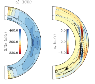
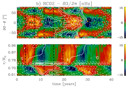
Figure 1: Left: (a) meridional distribution of the angular velocity and the meridional circulation for the model RC02. The profiles correspond to zonal and temporal averages over $\sim 10$ year during the steady phase of the simulation. Right: (b) time-latitude diagram for $r=0.95R_{\odot}$ (upper panel), and time-radius diagram for $30^{o}$ latitude (bottom panel) of $\delta\Omega(r,\theta,t)/2\pi=(2\pi\varpi)^{-1}(u_{\phi}(r,\theta,t)-\overline{u}_{\phi}(r,\theta))$. The continuous (dashed) white line contours depict the positive (negative) toroidal magnetic field strength also shown in Fig. 6b of Paper I.

In Fig. 1(b) a speed-up of the zonal flow at higher latitudes during the minimum of the toroidal field can be observed. This branch propagates toward the equator. When the magnetic field is strong at higher latitudes, there is a branch of less rapidly rotating plasma that also propagates toward the equator. At lower latitudes, the change between speed-up and slow-down occurs roughly when the toroidal field reverses polarity. In the tachocline, the field is stronger at the starting phase of the magnetic cycle. During this phase the zonal flow is accelerated (bottom panel of Fig. 1(b)). It decelerates during the declining and reversal stages of the cycle.

To look for a physical explanation for these features, we start by analyzing the angular momentum balance resulting from the different transport mechanisms. After multiplying the zonal component of the momentum equation (Eq. 3 in Paper 1) by $\varpi$, and then making a mean-field decomposition, we obtain the equation for the angular momentum evolution:

$$\frac{\partial({\rho}_{s}\overline{u}_{\phi})}{\partial t}=-\frac{1}{\varpi}\nabla\cdot\left(\varpi\left[\rho_{s}(\overline{u}_{\phi}+\varpi\Omega_{0})\overline{\bm{u}}_{\rm m}+\rho_{s}\overline{u_{\phi}^{\prime}{\bm{u}}^{\prime}_{\rm m}}-\frac{1}{\mu_{0}}\overline{B}_{\phi}\overline{{\bm{B}}}_{\rm p}-\frac{1}{\mu_{0}}\overline{b_{\phi}^{\prime}{\bm{b}}_{\rm p}^{\prime}}\right]\right),$$ (1)

where, $\overline{\bm{u}}_{\rm m}$, ${\bm{u}}^{\prime}_{\rm m}$, $\overline{\bm{B}}_{\rm p}$ and ${\bm{b}}^{\prime}_{\rm p}$ denote the mean and turbulent meridional ($r$ and $\theta$) components of the velocity and magnetic fields, respectively. Because the lhs of Eq. 1 is not in equilibrium but oscillates in time, the eight terms under the divergence in the rhs -

$${\cal F}_{r}^{\rm MC} = \rho_{s}\varpi(\overline{u}_{\phi}+\varpi\Omega_{0})\overline{u}_{r},$$ (2)

$${\cal F}_{\theta}^{\rm MC} = \rho_{s}\varpi(\overline{u}_{\phi}+\varpi\Omega_{0})\overline{u}_{\theta},$$

$${\cal F}_{r}^{\rm RS} = \rho_{s}\varpi\overline{{u}_{\phi}^{\prime}{u}_{r}^{\prime}},$$

$${\cal F}_{\theta}^{\rm RS} = \rho_{s}\varpi\overline{{u}_{\phi}^{\prime}{u}^{\prime}_{\theta}},$$

$${\cal F}_{r}^{\rm MT} = -\frac{\varpi}{\mu_{0}}\overline{B}_{\phi}\overline{B}_{r},$$

$${\cal F}_{\theta}^{\rm MT} = -\frac{\varpi}{\mu_{0}}\overline{B}_{\phi}\overline{B}_{\theta},$$

$${\cal F}_{r}^{\rm MS} = -\frac{\varpi}{\mu_{0}}\overline{{b}_{\phi}^{\prime}{b}_{r}^{\prime}},$$

$${\cal F}_{\theta}^{\rm MS} = -\frac{\varpi}{\mu_{0}}\overline{{b}_{\phi}^{\prime}{b}^{\prime}_{\theta}},$$

namely, the fluxes of angular momentum due to meridional circulation (MC), Reynold stresses (RS), the axisymmetric (or magnetic tension MT) and turbulent Maxwell stresses (MS) - should account for such variations. The net angular momentum transport is then computed (see Brun et al. 2004; Beaudoin et al. 2013) as

$$I_{r}(r)=\int_{0}^{\pi}{\cal F}_{r}(r,\theta)r^{2}\sin\theta d\theta$$ (3)

$$I_{\theta}(\theta)=\int_{r_{b}}^{r_{t}}{\cal F}_{\theta}(r,\theta)r\sin\theta dr,$$

where $r_{b}=0.61R_{\odot}$, $r_{t}=0.96R_{\odot}$ and:

$${\cal F}_{r}={\cal F}_{r}^{\rm MC}+{\cal F}_{r}^{\rm RS}+{\cal F}_{r}^{\rm MT}+{\cal F}_{r}^{\rm MS}$$ (4)

$${\cal F}_{\theta}={\cal F}_{\theta}^{\rm MC}+{\cal F}_{\theta}^{\rm RS}+{\cal F}_{\theta}^{\rm MT}+{\cal F}_{\theta}^{\rm MS}.$$

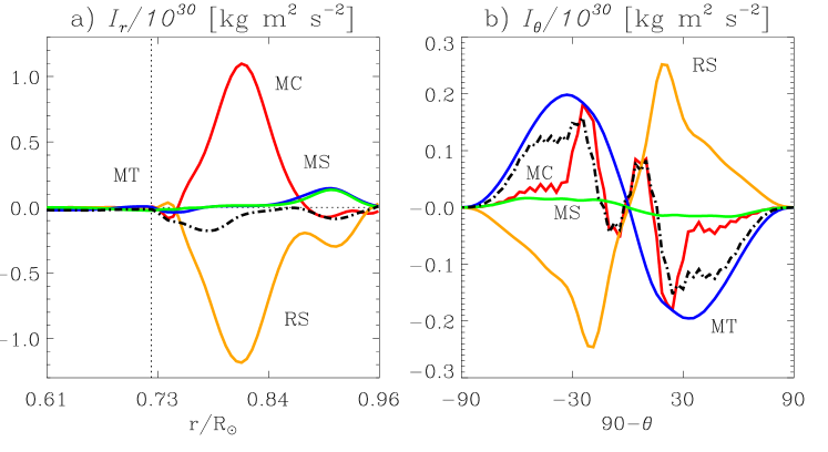
Figure 2: Integrated angular momentum fluxes for model RC02 as defined by Eqs. (2) to (4). The red, orange, blue, and green lines correspond to the MC (meridional circulation), RS (Reynolds stress), MT (magnetic tension), and MS (Maxwell stresses) fluxes, respectively. The black dot-dashed lines are the total contribution in each direction.

Fig. 2 shows the integrated radial (left) and latitudinal (right) profiles of the angular momentum fluxes of the rhs of Eq. 4. Red, orange, blue, and green lines correspond to the MC, RS, MT, and MS fluxes, respectively. Since the lhs of Eq. (1) is different from zero during the magnetic cycle, in order to investigate a steady state balance we average the integrated fluxes for two complete magnetic cycles. The black dotted-dashed lines correspond to the sum of all of the integrated magnetic fluxes in each direction. By interpreting the information in this figure, it is possible to disentangle the different contributions to the transport of angular momentum.

The radial transport shows a larger contribution from the Reynolds stress component, which is balanced by the MC term. It is evident from the black dotted-dashed line in Fig. 2(a) that the sum of the integrated fluxes balances well in the convection zone. The upper limit for the viscous contribution to the angular momentum transport, i.e., the residual of ${\cal F}_{r}$ (see Eq. 4), is less than 10% of the values of the RS or MC fluxes in this region.

Both magnetic contributions seem to be negligible in most of the domain except for the interface between the stable and the unstable layers and for the near-surface shear layer. In the stable region, the viscous angular momentum flux is significant and balances the magnetic fluxes. The amplitude of these components in the radiative zone is less than 2% of the value in the convection zone. However, it is sufficient for transporting angular momentum into the stable region, ultimately making this layer to rotate faster on average than the reference frame (Fig. 1(a)). Because periodic changes in the angular momentum transport in the radiative zone are solely due to the magnetic fluxes, it is clear that the TO in the radiative zone must have magnetic origin.

Figure 2(b) helps to explain the solar-like differential rotation pattern observed in Fig. 1(a). First of all, the dominant term is the Reynold stress flux, which is positive (negative) in the northern (southern) hemisphere. This means that the angular momentum transport is equatorward. The dominant RS is a robust feature of global models with solar-like differential rotation (e.g. Guerrero et al. 2013; Featherstone & Miesch 2015). Opposed to this transport are the meridional circulation, the magnetic tension and the Maxwell stress fluxes. The amplitude of the latitudinal integrated fluxes (Fig. 2(b)) is about 30% smaller than the radial fluxes, and the viscous contribution (which is of the same order as that in Fig. 2(a)) appears to be important for the latitudinal transport. Because at lower latitudes the RS and MT fluxes balance each other, the viscous flux clearly compensates the variation of the meridional circulation. At higher latitudes, the sum of the MC and MT fluxes should balance the RS flux. However, due to temporal variations of both quantities, they are not in balance. The sub-grid scale (SGS) viscous flux balances this difference. As shown later in Fig. 4, the variance of the RS flux over the cycle is minimal. This suggests that the TO are of magnetic origin. For instance, they may be driven directly through the large-scale magnetic torque, but also indirectly via the transport of angular momentum by meridional flow modulated by the magnetic cycle, as suggested by Beaudoin et al. (2013).

Next, we compare the meridional profiles of the torsional oscillations with those of the axial torques, $-\overline{\nabla\cdot\cal{F}}$, where $\cal{F}$ are the eight quantities of Eq. 2 (Fig 3). The columns, from left to right, correspond to the MC, RS, and MT torques, the total axial torque, and $\overline{\delta\Omega}$ as defined above, respectively. The rows correspond to four different time averages (of 4 years each) in four different phases of a full magnetic cycle. These phases starting at $t=3.5$ year are depicted by black dashed lines in Fig. 1(b). For the torques, the red and blue contours represent positive (entering into the page) and negative (out of the page) directions, respectively. We do not present $-\overline{\nabla\cdot\cal{F}_{\rm MS}}$, because its contribution is negligible in most of the domain. For the TO (rightmost panel), like in Fig. 1(b), the red (green) contour levels indicate a speed-up (slow-down) of the rotation. We notice that the meridional profiles of TO in different cycle phases also closely resemble the observations (see Fig. 8 of Howe et al. 2005, for comparison).

As discussed in the literature (e.g., Featherstone & Miesch 2015), the balance of these torques is responsible for the maintenance of the mean-flows. As expected from Fig. 2, $-\overline{\nabla\cdot\cal{F}_{\rm MC}}$ and $-\overline{\nabla\cdot\cal{F}_{\rm RS}}$ tend to balance each other in the bulk of the convection zone. Whenever the RS axial torque is negative (positive), it will induce a meridional flow away from (toward) the rotation axis. This explains well the two main MC cells at lower latitudes, the deeper cell being counterclockwise and the shallow one being clockwise (see e.g., Featherstone & Miesch 2015, for a complete analysis). Despite the fact that our simulation is MHD, the profiles of $-\overline{\nabla\cdot\cal{F}_{\rm MC}}$ and $-\overline{\nabla\cdot\cal{F}_{\rm RS}}$ compare well with those obtained by, e.g., Brun et al. (2011); Featherstone & Miesch (2015). Nevertheless, the profile of $-\overline{\nabla\cdot\cal{F}_{\rm RS}}$ presented here has negative values near the surface and at latitudes above $30^{o}$. As mentioned before, this negative torque is ultimately responsible for the formation of the NSSL (see also Miesch & Hindman 2011; Hotta et al. 2015).

The profile of $-\overline{\nabla\cdot\cal{F}_{\rm RS}}$ does not show significant changes during the magnetic cycle. On the other hand, $-\overline{\nabla\cdot\cal{F}_{\rm MC}}$ exhibits regions of strong periodically varying torque at the base of the convection zone and variations of its amplitude at the surface. These changes are a response to the magnetic torques, mainly to $-\overline{\nabla\cdot\cal{F}_{\rm MT}}$, which peaks at the rotational shear layers. The latitudinal distribution of $-\overline{\nabla\cdot\cal{F}_{\rm MT}}$ at the tachocline has positive values at higher latitudes and negative values at the equator. The change in amplitude of $-\overline{\nabla\cdot\cal{F}_{\rm MC}}$ and $-\overline{\nabla\cdot\cal{F}_{\rm MT}}$ seems to be associated with the TO presented in the rightmost column. This is reflected in the total axial torque (fourth column of Fig. 3) which in the first two phases, $\Delta t_{1}$ and $\Delta t_{2}$ shows bluish (negative torque) levels at higher latitudes, accounting for the slowed-down poles. During the two last phases, $\Delta t_{3}$ and $\Delta t_{4}$, $-\overline{\nabla\cdot\cal{F}_{\rm total}}$ has reddish (positive torque) levels at higher latitudes when the poles speed-up and the equator slows-down.

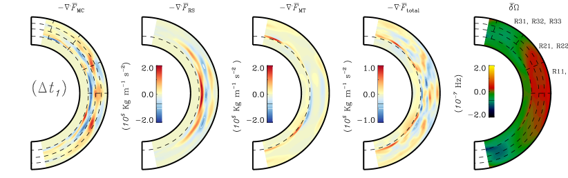
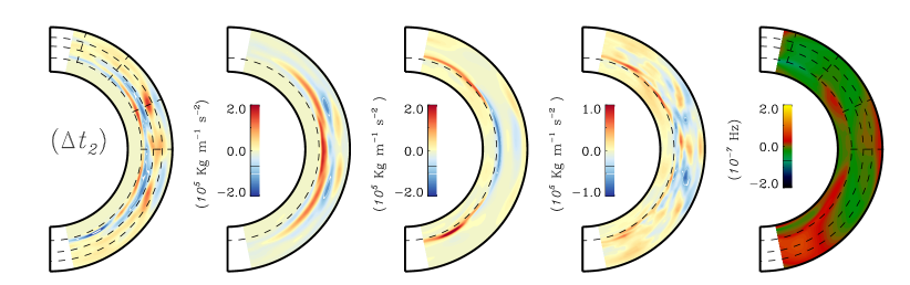
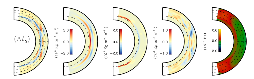
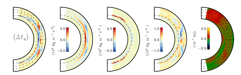
Figure 3: Meridional profiles of the total axial torques and $\overline{\delta\Omega}$ in four different time intervals corresponding to the different phases of the magnetic cycle depicted with black dashed lines in Fig. 1(b). For a better comparison with the available observational results, in the figure we present latitudes only up to $85^{o}$.

To explore the locality and causality issue more deeply, we have divided the first meridional quadrant of the domain into nine regions, which can be observed in the first panel of Fig. 3. The equatorial regions, R11, R12, and R13, span from $0^{o}\leq\theta<25^{o}$ latitude and $0.71\leq r/R_{\odot}<0.81$, $0.81\leq r/R_{\odot}<0.88$, and $0.88\leq r/R_{\odot}\leq 0.96$ in radius, respectively; intermediate latitude regions, R21, R22, and R23, span from $25^{o}\leq\theta<50^{o}$; and high latitude regions, R31, R32, and R33, span from $50^{o}\leq\theta<75^{o}$, all with the same radial extents. For each region we have computed the volume average of the axial torques but did not average in time, in order to study the time evolution of the four quantities and assess their relative importance. In the results, presented in Fig. 4, the time series lines follow the same color pattern as in Fig. 2, i.e., the red, orange, blue, and green lines correspond to the MC, RS, MT, and MS axial torques, respectively. These quantities are normalized to the maximum local value of $-\langle\nabla\cdot{\cal F}_{\rm MC}\rangle$ (the angular brackets indicate volume averages over each reagion). The black lines correspond to $\langle\delta\Omega\rangle$ normalized to $10^{-7}$ Hz. The gray shaded region indicates the four time intervals presented in Fig. 3. These time series explain the origin of the TO.

In region R31 (pole-bottom, Fig. 4(a)), there is a clear correlation between the MT torque and $\langle\delta\Omega\rangle$. At $\Delta t_{1}$ the positive MT torque is decreasing while the negative MC torque increases, balancing the angular momentum. The amplitude of the MT torque is higher, leading to a slow-down of the angular velocity. In $\Delta t_{2}$ the MT torque quickly increases and $\Omega$ speeds-up in spite of the decline of MC. The phases $\Delta t_{3}$ and $\Delta t_{4}$ correspond to the maximum (minimum) and to the decline (rise) of the MT (MC) torque, respectively, and are associated to the slow-down of $\Omega$. The phase relation between the blue and the black lines leaves no doubt that the MT causes the TO. It is remarkable that, in this latitude range, the TO pattern remains more or less the same in radius, with only minor changes of the amplitude. In region R32 (pole-bulk, panel (b)) the RS torque is negative and MC is positive. The latter shows variations that seem to follow the TO. In R33 (pole-top, panel (c)), the MC torque is mostly positive and clearly follows the TO, becoming negative in its minima. The MT torque in this zone is due to the magnetic field generated in the NSSL and anti-correlates with the TO which seems to conserve the imprints produced in it by the MT torque at the bottom layers, in R31.

In the intermediate regions R21, R22, and R23 (Fig. 4(d)-(f)), the torques exhibit less variation while $\langle\delta\Omega\rangle$ conserves roughly the same oscillation pattern but with some phase delay (of about $\pi/4$) and smaller amplitudes than that acquired at higher latitudes. In R22 and R23, the changes from positive to negative occur at the beginning of $\Delta t_{2}$, i.e., 4 years after the transitions in R32 and R33. This is a consequence of the migration of the positive (negative) MT toward the equator (poles) observed in Fig. 3. This migration explains the propagation of the TO.

Finally, in R11 (equator-bottom, panel (g)), the time series indicate a similar behavior to what is observed in the region R31, i.e., there is a clear correlation between the MT torque and the TO. Besides, we note that in this case the MT and MC torques are negative and, evidently, oscillate in anti-phase. The sign change of the MT torque from the poles to the equator reflects the fact that, in the dynamo, the mean toroidal and poloidal fields have certain phase difference. Opposite to region R31, in R11 $\langle\delta\Omega\rangle$ is positive during $\Delta t_{1}$ (see also the two upper rows of Fig. 3). It also has lower amplitude. The evolution of the TO curve follows that of the MT torque, i.e., it rises slowly and declines rapidly. The observed correlation suggests that this equatorial oscillation is driven by the MT. It also propagates upwards, conserving a similar shape in regions R12 and R13. In panel (i), region R13 (equator-top), the MC torque oscillates with a large amplitude which does not seem to be compensated by any other torque. This imbalance (actually seen also in R33 and R23) is expected, as this is the fraction of the domain where the numerical viscous contribution to the angular momentum transport is relevant (see Fig. 2a). Once again, the MC oscillations seem to be connected to the TO and unrelated to any other torque variation in the same region.

Besides the changes with the periodicity of the magnetic cycle, the MC torque also depicts erratic short term fluctuations. On the other hand, the evolution of $\langle\delta\Omega\rangle$ is less noisy, which is also the case for the magnetic torque $-\langle\nabla\cdot{\cal F}_{\rm MT}\rangle$. This supports the argument that the TO are induced by the MT at the base of the convection zone. Thus, the observed variation of the MC is a by-product of the periodic speed-up and slow-down of the zonal flows. Note that a complete study on the meridional flow changes across the cycle relies not only on the zonal Reynolds stresses (Eq. 2) but also on its meridional components (Passos et al. 2016, in preparation).

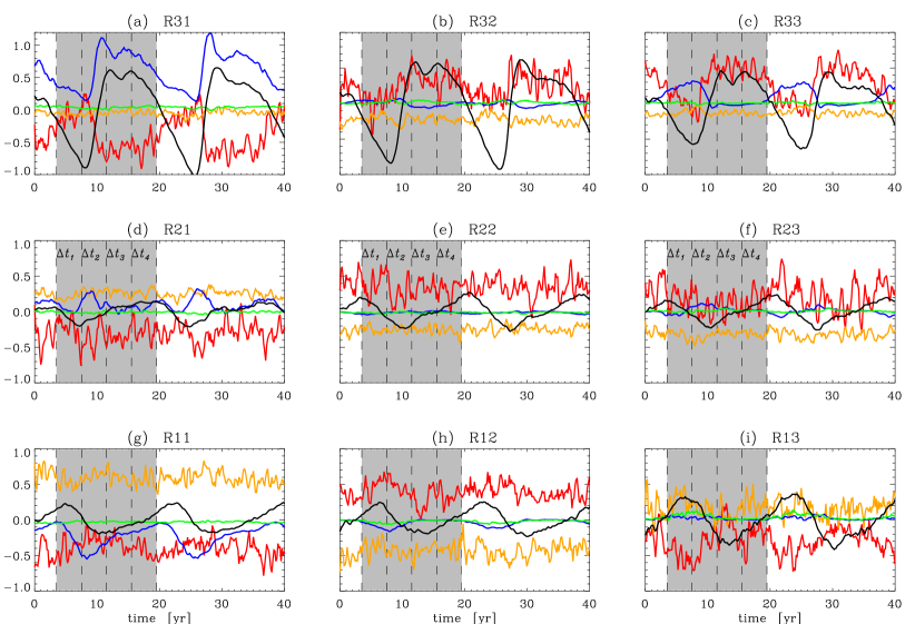
Figure 4: Time evolution of the axial torques computed for different latitudinal and radial regions labeled in the upper row of Fig. 3. Red, orange, blue and green lines correspond to the MC, RS, MT and MS axial torques normalized to the local maximum value of $\langle\nabla\cdot\cal{F}_{\rm MC}\rangle$. The black line shows the evolution of $\langle\delta\Omega\rangle$ normalized to $10^{-7}$. The angular brackets mean volume averages over each region.

4 Discussion and Conclusions

Besides affecting the average profile of the differential rotation, the magnetic feedback generates TO in a periodic convective dynamo model (model RC02). We have demonstrated that the origin of these oscillations in our simulation is due to the magnetic torque induced by the strong large-scale magnetic fields at the model’s tachocline. The temporal evolution of the axial torques in different regions of our simulation domain suggests that the two branches of TO are directly driven by the magnetic tension (MT) at the base of the convection zone. This perturbation propagates upwards up to the surface. The sign difference between the poles and the equator, as well as the latitudinal migration of the TO, is explained by the phase delay between the MT at higher and lower latitudes.

Despite the amplitude of the TO in our simulations being higher than the observed amplitude in the Sun, we notice morphological similarities with the observations for both the TO and the variation of the MC. Our results support the hypothesis that it is the magnetic field that modifies the meridional circulation during the solar cycle. This is in contrast to the idea that the meridional flow governs the solar cycle, as proposed by flux-transport dynamo models (e.g., Nandy et al. 2011). In our results, the variations of the MC appear correlated with variations of the angular velocity, which, in turn, are driven by the deep dynamo-generated magnetic field.

The distribution of the magnetic field below the photosphere is an open question and is relevant for the understanding of the solar dynamo. It should be addressed with the correct understanding of the TO (e.g., Antia et al. 2013). This work represents a step forward in that direction.

References

- Antia & Basu (2001) Antia, H. M., & Basu, S. 2001, ApJ, 559, L67
- Antia et al. (2013) Antia, H. M., Chitre, S. M., & Gough, D. O. 2013, MNRAS, 428, 470
- Beaudoin et al. (2013) Beaudoin, P., Charbonneau, P., Racine, E., & Smolarkiewicz, P. K. 2013, Sol. Phys., 282, 335
- Brun et al. (2004) Brun, A. S., Miesch, M. S., & Toomre, J. 2004, ApJ, 614, 1073
- Brun et al. (2011) —. 2011, ApJ, 742, 79
- Covas et al. (2004) Covas, E., Moss, D., & Tavakol, R. 2004, A&A, 416, 775
- Covas et al. (2000) Covas, E., Tavakol, R., Moss, D., & Tworkowski, A. 2000, A&A, 360, L21
- Featherstone & Miesch (2015) Featherstone, N. A., & Miesch, M. S. 2015, ApJ, 804, 67
- Guerrero et al. (2016) Guerrero, G., Smolarkiewicz, P. K., de Gouveia Dal Pino, E. M., Kosovichev, A. G., & Mansour, N. N. 2016, ApJ, 819, 104
- Guerrero et al. (2013) Guerrero, G., Smolarkiewicz, P. K., Kosovichev, A. G., & Mansour, N. N. 2013, ApJ, 779, 176
- Hotta et al. (2015) Hotta, H., Rempel, M., & Yokoyama, T. 2015, ApJ, 798, 51
- Howard & Labonte (1980) Howard, R., & Labonte, B. J. 1980, ApJ, 239, L33
- Howe (2009) Howe, R. 2009, Living Reviews in Solar Physics, 6, 1
- Howe et al. (2005) Howe, R., Christensen-Dalsgaard, J., Hill, F., et al. 2005, ApJ, 634, 1405
- Howe et al. (2000) Howe, R., Komm, R., & Hill, F. 2000, Sol. Phys., 192, 427
- Kleeorin & Ruzmaikin (1981) Kleeorin, N. I., & Ruzmaikin, A. A. 1981, Solar Physics, 131, 211
- Komm et al. (2015) Komm, R., González Hernández, I., Howe, R., & Hill, F. 2015, Sol. Phys., 290, 3113
- Komm et al. (2014) Komm, R., Howe, R., González Hernández, I., & Hill, F. 2014, Sol. Phys., 289, 3435
- Kosovichev & Schou (1997) Kosovichev, A. G., & Schou, J. 1997, ApJ, 482, L207
- Kosovichev & Zhao (2016) Kosovichev, A. G., & Zhao, J. 2016, Reconstruction of Solar Subsurfaces by Local Helioseismology, ed. J.-P. Rozelot & C. Neiner (Cham: Springer International Publishing), 25–41
- Margolin et al. (2006) Margolin, L. G., Rider, W. J., & Grinstein, F. F. 2006, Journal of Turbulence, 7, N15
- Miesch & Hindman (2011) Miesch, M. S., & Hindman, B. W. 2011, ApJ, 743, 79
- Nandy et al. (2011) Nandy, D., Muñoz-Jaramillo, A., & Martens, P. C. H. 2011, Nature, 471, 80
- Passos et al. (2016) Passos, D., Miesch, M., Charbonneau, P., & Guerrero, G. 2016, In preparation
- Piotrowski et al. (2009) Piotrowski, Z. P., Smolarkiewicz, P. K., Malinowski, S. P., & Wyszogrodzki, A. A. 2009, Journal of Computational Physics, 228, 6268
- Prusa et al. (2008) Prusa, J. M., Smolarkiewicz, P. K., & Wyszogrodzki, A. A. 2008, Comput. Fluids, 37, 1193
- Rempel (2007) Rempel, M. 2007, ApJ, 655, 651
- Smolarkiewicz & Charbonneau (2013) Smolarkiewicz, P. K., & Charbonneau, P. 2013, J. Comput. Phys., 236, 608
- Spruit (2003) Spruit, H. C. 2003, Sol. Phys., 213, 1
- Toomre et al. (2000) Toomre, J., Christensen-Dalsgaard, J., Howe, R., et al. 2000, Sol. Phys., 192, 437
- Vorontsov et al. (2002) Vorontsov, S. V., Christensen-Dalsgaard, J., Schou, J., Strakhov, V. N., & Thompson, M. J. 2002, Science, 296, 101
- Yoshimura (1981) Yoshimura, H. 1981, ApJ, 247, 1102
- Zhao et al. (2014) Zhao, J., Kosovichev, A. G., & Bogart, R. S. 2014, ApJ, 789, L7