Determination of magic wavelengths for the $7s~{}{{}^{2}}S_{1/2}-7p~{}{{}^{2}}P_{3/2,1/2}$ transitions in Fr atom

Abstract

Magic wavelengths ($\lambda_{\rm{magic}}$) for the $7S_{1/2}-7P_{1/2,3/2}$ transitions (D-lines) in Fr were reported by Dammalapati et al. in [Phys. Rev. A 93, 043407 (2016)]. These $\lambda_{\rm{magic}}$ were determined by plotting dynamic polarizabilities ($\alpha$) of the involved states with the above transitions against a desired range of wavelength. Electric dipole (E1) matrix elements listed in [J. Phys. Chem. Ref. Data 36, 497 (2007)], from the measured lifetimes of the $7P_{1/2,3/2}$ states and from the calculations considering core-polarization effects in the relativistic Hartree-Fock (HFR) method, were used to determine $\alpha$. However, contributions from core correlation effects and from the E1 matrix elements of the $7P-7S$, $7P-8S$ and $7P-6D$ transitions to $\alpha$ of the $7P$ states were ignored. In this work, we demonstrate importance of these contributions and improve accuracies of $\alpha$ further by replacing the E1 matrix elements taken from the HFR method by the values obtained employing relativistic coupled-cluster theory. Our static $\alpha$ are found to be in excellent agreement with the other available theoretical results; whereas substituting the E1 matrix elements used by Dammalapati et al. give very small $\alpha$ values for the $7P$ states. Owing to this, we find disagreement in $\lambda_{\rm{magic}}$ reported by Dammalapati et al. for linearly polarized light; especially at wavelengths close to the D-lines and in the infrared region. As a consequence, a $\lambda_{\rm{magic}}$ reported at 797.75 nm which was seen supporting a blue detuned trap in their work is now estimated at 771.03 nm and is supporting a red detuned trap. Also, none of our results match with the earlier results for circularly polarized light. Moreover, our static values of $\alpha$ will be very useful for guiding experiments to carry out their measurements.

I Introduction

Being the heaviest alkali atom, Fr atom is considered for measuring electric dipole moment (EDM) due to parity and time reversal symmetries Sakemi et al. (2011); Inoue et al. (2015); Mukherjee and Pal (1989), parity nonconservation (PNC) effect in the $7s\ ^{2}S_{1/2}\rightarrow 8s\ ^{2}S_{1/2}$ transition due to neutral weak interaction Stancari et al. (2007); Sahoo (2010) and PNC effect among the hyperfine transitions in the ground state Gomez et al. (2007) and in the $7s\ ^{2}S_{1/2}\rightarrow 6d\ ^{2}D_{5/2}$ transition due to the nuclear anapole moment Sahoo et al. (2016). Recent theoretical studies on hyperfine structures in ²¹⁰Fr and ²¹²Fr demonstrate inconsistencies between the theoretically evaluated and measured hyperfine structure constants of few excited states Sahoo et al. (2015). The hyperfine structure constants and lifetimes of the $6d\ ^{2}D_{3,5/2}$ states of Fr, which are important for PNC studies Sahoo et al. (2015); Sahoo and Das (2015), have not been measured yet. Also, suggestion to measure hyperfine splitting in the suitable transitions to observe nuclear octupole moment of its ²¹¹Fr isotope have been made Sahoo (2015). To carry out high precision measurements for all the above mentioned vital studies, it is indispensable to conduct experiments on Fr atoms in an environment where they are least affected by external perturbations. In such scenario, performing experiments by cooling and trapping Fr atoms using lasers can be advantageous. To estimate the induced Stark shifts in the energy levels due to the applied lasers, knowledge about precise values of polarizabilities is necessary. There are no experimental results on polarizabilities in Fr available yet, while only a few theoretical results are reported.

Techniques to produce Fr atoms and trapping them in a magneto-optic trap (MOT) have already been demonstrated Simsarian et al. (1998); Atutov et al. (2015). Similar to other alkali atoms D-lines in Fr atom are used for laser cooling and trapping experiments, which leads to the easy accessibility of this atom for its application in probing new physics of fundamental particles Dammalapati et al. (2016); Phillips (1998); Simsarian et al. (1996). Therefore, it is certainly attainable to develop cooling and trapping techniques for the Fr atoms in near future. It is worth mentioning here that recently there have been proposals suggesting to adopt these methodologies to measure PNC and EDM in the Fr atom Sahoo et al. (2016); Inoue et al. (2015). However, when lasers are applied to the atoms, the Stark shifts experienced by the energy levels cause large systematics to carry out high precision measurements of any spectroscopic properties. One of the most innovative ways to circumvent this problem is to trap the atoms at the magic wavelengths ($\rm\lambda_{magic}$) at which differential Stark shift of a transition is effectively nullified. The concept of $\rm\lambda_{magic}$ was first introduced by Katori et al. for its application in the optical atomic clocks Katori et al. (1999). In fact, $\rm\lambda_{magic}$ of the $6s~{}{{}^{2}}S_{1/2}$-$6p~{}{{}^{2}}P_{3/2}$ transition in Cs has been measured by Mckeever et al. at 935.6 nm McKeever et al. (2003) using linearly polarized light. In our previous works, we have also theoretically determined $\rm\lambda_{magic}$ of D-lines of the lighter alkali atoms for both linearly and circularly polarized light Arora et al. (2007); Arora and Sahoo (2012); Sahoo and Arora (2013); Singh et al. (2016a, b). With the same objective, Dammalapati et al. Dammalapati et al. (2016) have recently identified $\rm\lambda_{magic}$ for the $7S_{1/2}-7P_{1/2,3/2}$ and $7S_{1/2}-8S_{1/2}$ transitions in Fr considering both linearly and circularly polarized light. On this rationale, they have used transition rates compiled by Sansonetti in Ref. Sansonetti (2007) to calculate the required dynamic dipole polarizabilities. Few of these transition probabilities quoted by Sansonetti were extracted from the measurements of the lifetimes of the $7P_{1/2,3/2}$ states of Fr, while the remaining data were taken from the calculations, based on the relativistic Hartree-Fock (HFR) method accounting only the core-polarization effects, carried out by Biemont et al. Biemont et al. (1998). However, these calculations of polarizabilities completely ignore contributions coming from the correlations due to the core electrons (known as core correlation contribution), which are about 6% in the evaluation of the static values of polarizabilities as has been demonstrated later, and correlations among the core and valence electrons (referred in the literature as core-valence correlation contribution), and from the high-lying transitions (tail contribution) involving states above $n=20$, for the principal quantum number $n$. Most importantly, Dammalapati et al. have not considered the contributions from the $7P-7S$, $7P-8S$ and $7P-6D$ transitions in their calculations of the dynamic polarizabilities of the $7P_{1/2,3/2}$ states. As shown in this work subsequently, contributions from these states are more than 80% to the static polarizability values of the $7P_{1/2,3/2}$ states. Therefore, it is imperative to determine $\rm\lambda_{magic}$ of the important D-lines of the Fr atom more precisely by determining polarizabilities of the atomic states more accurately.

We pursue this work intending to improve evaluation of $\rm\lambda_{magic}$ over the previously reported values for both linearly and circularly polarized light by including the core, core-valence and tail contributions and also accounting contributions from the $7P-7S$, $7P-8S$ and $7P-6D$ transitions. In addition to this, we use more accurate values of the electric dipole (E1) matrix elements for the higher excited states from a relativistic coupled-cluster (RCC) theory as compared to the values used from a lower order many-body method in Dammalapati et al. (2016). In order to validate our results, we have also estimated static dipole polarizability values of the ground and $7P_{1/2,3/2}$ states and compare them against the other available high precision calculations. In order to demonstrate importance of inclusion of the appended contributions in the evaluation of the polarizabilities and also to find out possible reason for the discrepancies in the $\rm\lambda_{magic}$ from both the works, we present contributions to the static polarizabilities from various transitions, core correlations and core-valence correlations explicitly. We also estimate the static polarizability values of the above states obtained exclusively using the E1 matrix elements considered by Dammalapati et al. and compare them with the other theoretical results.

Table 1: Contributions from reduced E1 matrix elements (given as $d$), core correlation and core-valence correlation to the static polarizabilities of the $7S_{1/2}$, $7P_{1/2}$ and $7P_{3/2}$ states of Fr atom. The final results are compared with the previously estimated results. The results marked ‘*’ are calculated using the reduced E1 matrix elements (taken from Ref. Sansonetti (2007)) which are considered in Ref. Dammalapati et al. (2016) to determine $\rm\lambda_{magic}$. All the values are given in atomic units (a.u.).

$7S_{1/2}$ state			$7P_{1/2}$ state			$7P_{3/2}$ state
Transition	$d$	$\alpha_{n}^{(0)}$	Transition	$d$	$\alpha_{n}^{(0)}$	Transition	$d$	$\alpha_{n}^{(0)}$	$\alpha_{n}^{(2)}$
$7S_{1/2}-7P_{1/2}$	4.277	109.36	$7P_{1/2}-7S_{1/2}$	4.277	-109.36	$7P_{3/2}-7S_{1/2}$	5.898	-91.39	91.39
$7S_{1/2}-8P_{1/2}$	0.33	0.35	$7P_{1/2}-8S_{1/2}$	4.27	177.79	$7P_{3/2}-8S_{1/2}$	7.52	355.67	-355.67
$7S_{1/2}-9P_{1/2}$	0.11	0.03	$7P_{1/2}-9S_{1/2}$	1.02	5.67	$7P_{3/2}-9S_{1/2}$	1.39	6.02	-6.02
$7S_{1/2}-10P_{1/2}$	0.06	0.01	$7P_{1/2}-10S_{1/2}$	0.54	1.33	$7P_{3/2}-10S_{1/2}$	0.71	1.28	-1.28
$7S_{1/2}-11P_{1/2}$	0.04	$\sim$0	$7P_{1/2}-11S_{1/2}$	0.35	0.51	$7P_{3/2}-11S_{1/2}$	0.45	0.47	-0.47
$7S_{1/2}-7P_{3/2}$	5.898	182.77	$7P_{1/2}-6D_{3/2}$	7.45	1017.03	$7P_{3/2}-6D_{3/2}$	3.44	187.72	150.18
$7S_{1/2}-8P_{3/2}$	0.95	2.79	$7P_{1/2}-7D_{3/2}$	3.27	65.15	$7P_{3/2}-7D_{3/2}$	2.07	15.19	12.15
$7S_{1/2}-9P_{3/2}$	0.44	0.52	$7P_{1/2}-8D_{3/2}$	1.79	15.26	$7P_{3/2}-8D_{3/2}$	1.00	2.67	2.14
$7S_{1/2}-10P_{3/2}$	0.28	0.19	$7P_{1/2}-9D_{3/2}$	1.17	5.86	$7P_{3/2}-9D_{3/2}$	0.62	0.91	0.73
$7S_{1/2}-11P_{3/2}$	0.18	0.08	$7P_{1/2}-10D_{3/2}$	0.84	2.86	$7P_{3/2}-10D_{3/2}$	0.44	0.43	0.35
						$7P_{3/2}-6D_{5/2}$	10.53	1618.72	-323.74
						$7P_{3/2}-7D_{5/2}$	5.91	122.74	-24.55
						$7P_{3/2}-8D_{5/2}$	2.91	22.57	-4.51
						$7P_{3/2}-9D_{5/2}$	1.83	7.95	-1.59
						$7P_{3/2}-10D_{5/2}$	1.27	3.60	-0.72
Main($\rm\alpha_{n,v}$)		296.10	Main($\rm\alpha_{n,v}$)		1182.10	Main($\rm\alpha_{n,v}$)		2254.56	-461.62
Tail($\rm\alpha_{n,v}$)		1.26	Tail($\rm\alpha_{n,v}$)		22.89	Tail($\rm\alpha_{n,v}$)		29.15	-5.24
$\rm\alpha_{n,cv}$		-0.95	$\rm\alpha_{n,cv}$		$\sim$0	$\rm\alpha_{n,cv}$		$\sim$0	$\sim 0$
$\rm\alpha_{n,c}$		20.4	$\rm\alpha_{n,c}$		20.4	$\rm\alpha_{n,c}$		20.4
Total		316.81	Total		1225.39	Total		2304.10	-466.86
Others		317.8(2.4) Derevianko et al. (1999)	Others		1106 Wijngaarden and Xia (1999)	Others		2102.6 Wijngaarden and Xia (1999)	-402.76 Wijngaarden and Xia (1999)
		315.2 Lim et al. (2005)			57.23*			98.57*	63.23*
		289.8*

II Theory

The Stark shift in the energy level of an atom in state $|\gamma_{n}J_{n}M_{J_{n}}\rangle$ placed in an uniform oscillating electric field $\mbox{\boldmath${\cal E}$}(t)=\frac{1}{2}{\cal E}\hat{\mbox{\boldmath$\varepsilon$}}e^{-\iota\omega t}+c.c.$, with ${\cal E}$ being the amplitude, $\hat{\mbox{\boldmath$\varepsilon$}}$ is the polarization vector of the electric field and $c.c.$ referring to the complex conjugate of the former term, oscillating at frequency $\omega$ is given by Bonin and Kresin (1997); Manakov et al. (1986); Beloy (2009)

$$\Delta E_{n}=-\frac{1}{4}\alpha_{n}(\omega){\cal E}^{2},$$ (1)

where, $\alpha_{n}(\omega)$ is known as the frequency dependent dipole polarizability, and is expressed as

$$\alpha_{n}(\omega) = -[\langle\gamma_{n}J_{n}M_{J_{n}}|(\hat{\mbox{\boldmath$\varepsilon$}}^{*}\cdot{\bf D})R_{n}^{+}(\omega)(\hat{\mbox{\boldmath$\varepsilon$}}\cdot{\bf D})$$ (2)

$$+ (\hat{\mbox{\boldmath$\varepsilon$}}\cdot{\bf D})R_{n}^{-}(\omega)(\hat{\mbox{\boldmath$\varepsilon$}}^{*}\cdot{\bf D})|\gamma_{n}J_{n}M_{J_{n}}\rangle],$$

where ${\bf D}=D\hat{\bf r}=-e\sum_{j}{\bf r}_{j}$ is the electric dipole (E1) operator with position of an $j^{th}$ electron ${\bf r}_{j}$ and the projection operators $R_{n}^{\pm}(\omega)$ are given by

$$R_{n}^{\pm}(\omega)=\sum_{k}\frac{|\gamma_{k}J_{k}M_{J_{k}}\rangle\langle\gamma_{k}J_{k}M_{J_{k}}|}{E_{n}-E_{k}\pm\omega}.$$ (3)

In the above expressions, $E_{n}$ and $J_{n}$ is the energy and angular momentum of the state $|\Psi_{n}\rangle$( denoted by $|\gamma_{n}J_{n}M_{J_{n}}\rangle$ in above expression), respectively, and sum over $k$ represents all possible allowed intermediate states $|\Psi_{k}\rangle$( denoted by $|\gamma_{k}J_{k}M_{J_{k}}\rangle$ in above expression) with $E_{k}$ and $J_{k}$ being the corresponding energies and angular momenta. $M_{J_{n}}$ and $M_{J_{k}}$ are the magnetic components of corresponding angular momenta. $\gamma_{n}$ and $\gamma_{k}$ include all the remaining quantum numbers of the corresponding state. Since D is a vector operator, we obtain three terms resulting from the scalar, vector and tensor components, respectively. Thus, it can be given as

$$\alpha_{n}(\omega)=C_{0}\alpha_{n}^{(0)}(\omega)+C_{1}\alpha_{n}^{(1)}(\omega)+C_{2}\alpha_{n}^{(2)}(\omega),$$ (4)

where $\alpha_{n}^{(0)}$, $\alpha_{n}^{(1)}$ and $\alpha_{n}^{(2)}$ are known as scalar, vector and tensor polarizabilities. In a sum-over-states approach, it yields

$$\alpha_{n}^{(0)}(\omega)=\sum_{k\neq n}W_{n}^{(0)}\left[\frac{|\langle\gamma_{n}J_{n}||{\bf D}||\gamma_{k}J_{k}\rangle|^{2}}{E_{n}-E_{k}+\omega}+\frac{|\langle\gamma_{n}J_{n}||{\bf D}||\gamma_{k}J_{k}\rangle|^{2}}{E_{n}-E_{k}-\omega}\right],$$ (5)

$$\alpha_{n}^{(1)}(\omega)=\sum_{k\neq n}W_{n,k}^{(1)}\left[\frac{|\langle\gamma_{n}J_{n}||{\bf D}||\gamma_{k}J_{k}\rangle|^{2}}{E_{n}-E_{k}+\omega}-\frac{|\langle\gamma_{n}J_{n}||{\bf D}||\gamma_{k}J_{k}\rangle|^{2}}{E_{n}-E_{k}-\omega}\right],$$ (6)

and

$$\alpha_{n}^{(2)}(\omega)=\sum_{k\neq n}W_{n,k}^{(2)}\left[\frac{|\langle\gamma_{n}J_{n}||{\bf D}||\gamma_{k}J_{k}\rangle|^{2}}{E_{n}-E_{k}+\omega}+\frac{|\langle\gamma_{n}J_{n}||{\bf D}||\gamma_{k}J_{k}\rangle|^{2}}{E_{n}-E_{k}-\omega}\right]$$ (7)

with the coefficients

$$W_{n}^{(0)} = -\frac{1}{3(2J_{n}+1)},$$ (8)

$$W_{n,k}^{(1)} = -\sqrt{\frac{6J_{n}}{(J_{n}+1)(2J_{n}+1)}}$$ (12)

$$\times(-1)^{J_{n}+J_{k}+1}\left\{\begin{array}[]{ccc}J_{n}&1&J_{n}\\ 1&J_{k}&1\end{array}\right\},$$

and

$$W_{n,k}^{(2)} = 2\sqrt{\frac{5J_{n}(2J_{n}-1)}{6(J_{n}+1)(2J_{n}+3)(2J_{n}+1)}}$$ (15)

$$\times(-1)^{J_{n}+J_{k}+1}\left\{\begin{array}[]{ccc}J_{n}&2&J_{n}\\ 1&J_{k}&1\end{array}\right\},$$

for $\langle\gamma_{n}J_{n}||{\bf D}||\gamma_{k}J_{k}\rangle$ being the electric dipole (E1) reduced matrix elements. The values of $C_{0}$, $C_{1}$ and $C_{2}$ coefficients in the above expressions depends on polarization of the electric field. In a number of applications oscillating electric fields produced by lasers with different choice of polarization are used depending on the suitability of an experimental geometry, but most commonly linearly and circularly polarized electric fields are considered. For linearly polarized light, one gets Manakov et al. (1986)

$$C_{0}=1,\ \ \ C_{1}=0,\ \ \ \text{and}\ \ \ C_{2}=\frac{3M_{J}^{2}-J_{n}(J_{n}+1)}{J_{n}(2J_{n}-1)}$$ (16)

for the magnetic component $M_{J}$ of $J_{n}$. Here, it is assumed that the quantization axis is along the direction of polarization vector. Similarly, for circularly polarized light it corresponds to

$$C_{0}=1,\ \ C_{1}=\frac{AM_{J}}{2J_{n}},\ \ \text{and}\ \ C_{2}=-\frac{3M_{J}^{2}-J_{n}(J_{n}+1)}{2J_{n}(2J_{n}-1)},$$ (17)

where $A$ is known as the degree of circular polarization which possess the values $1$ and $-1$ for the right handed and left handed circularly polarized electric field, respectively and it is assumed in this case that the direction of quantization is along the wave vector.

The differential Stark shift of a transition $|\Psi_{i}\rangle\rightarrow|\Psi_{f}\rangle$ between an initial state $|\Psi_{i}\rangle$ to a final state $|\Psi_{f}\rangle$ is the difference between the Stark shifts of these states and is given by

$$\delta(\Delta E)_{if}(\omega) = \Delta E_{i}(\omega)-\Delta E_{f}(\omega)$$ (18)

$$= -\frac{1}{4}\left[\alpha_{i}(\omega)-\alpha_{f}(\omega)\right]{\cal E}^{2}.$$

Differential stark shift between two states for linearly polarized light can be expressed as

$$\delta(\Delta E)_{if}(\omega) = -\frac{1}{4}\big{[}\big{\{}\alpha_{i}^{(0)}(\omega)-\alpha_{f}^{(0)}(\omega)\big{\}}+$$ (19)

$$\big{\{}\frac{3M_{J_{i}}^{2}-J_{i}(J_{i}+1)}{J_{i}(2J_{i}-1)}\alpha_{i}^{(2)}(\omega)-$$

$$\frac{3M_{J_{f}}^{2}-J_{f}(J_{f}+1)}{J_{f}(2J_{f}-1)}\alpha_{f}^{(2)}(\omega)\big{\}}\big{]}{\cal E}^{2}$$

Similarly, differential stark shift between two states ($|\Psi_{i}\rangle$ and $|\Psi_{f}\rangle$) using circularly polarized light can be written as

$$\delta(\Delta E)_{if}(\omega) = -\frac{1}{4}\big{[}\big{\{}\alpha_{i}^{(0)}(\omega)-\alpha_{f}^{(0)}(\omega)\big{\}}+$$ (20)

$$A\big{\{}\frac{M_{J_{i}}}{2J_{i}}\alpha_{i}^{(1)}(\omega)-\frac{M_{J_{f}}}{2J_{f}}\alpha_{f}^{(1)}(\omega)\big{\}}-$$

$$\frac{1}{2}\big{\{}\frac{3M_{J_{i}}^{2}-J_{i}(J_{i}+1)}{J_{i}(2J_{i}-1)}\alpha_{i}^{(2)}(\omega)-$$

$$\frac{3M_{J_{f}}^{2}-J_{f}(J_{f}+1)}{J_{f}(2J_{f}-1)}\alpha_{f}^{(2)}(\omega)\big{\}}\big{]}{\cal E}^{2}$$

Here, $A=1$ when right circularly polarized light is used and $A=-1$ when left circularly polarized light is used. For a $\omega$ value at which $\delta(\Delta E)_{if}(\omega)$ is zero, the corresponding wavelength is a $\rm\lambda_{magic}$. Equivalently, it means finding out where the condition $\alpha_{i}(\omega)=\alpha_{f}(\omega)$ is satisfied for amplitude ${\cal E}$.

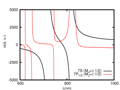
Figure 1: (Color online) Dynamic polarizabilities (in a.u.) for the $7S_{1/2}$ and $7P_{1/2}$ states of Fr in the wavelength range 600-1000 nm for linearly polarized light .

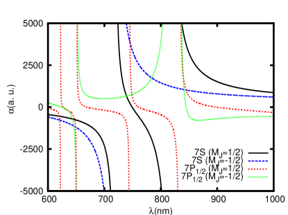
Figure 2: (Color online) Dynamic polarizabilities (in a.u.) for the $7S_{1/2}$ and $7P_{1/2}$ states of Fr in the wavelength range 600-1000 nm for left circularly polarized light(A=-1).

III Method of Evaluation for Polarizability

To evaluate atomic wave functions of the ground and many low-lying excited states having a common closed core configuration $[6p^{6}]$ and a valence orbital (say, $n$) in Fr in the RCC theory framework, we first calculate the Dirac-Fock (DF) wave function ($|\Phi_{0}\rangle$) for the closed core and then define a new working DF wave function of the entire state artificially as $|\Phi_{n}\rangle=a_{n}^{\dagger}|\Phi_{0}\rangle$, appending the corresponding valence orbital $n$. In this procedure, evaluation of the exact atomic wave functions of the respective states requires incorporating the correlations among the electrons within $|\Phi_{0}\rangle$ that is referred to as core correlation, correlations effectively seen by only the valence electron of $|\Phi_{n}\rangle$ which is termed as valence correlation, and the correlations between the core electrons with the valence electron $v$ giving rise to core-valence correlation contributions. Using the wave operator formalism, one can express these wave functions accounting the above mentioned correlations individually as Arora et al. (2012); Kaur et al. (2015)

$$|\Psi_{n}\rangle = a_{n}^{\dagger}\Omega_{c}|\Phi_{0}\rangle+\Omega_{cv}|\Phi_{n}\rangle+\Omega_{v}|\Phi_{n}\rangle,$$ (21)

where $\Omega_{c}$, $\Omega_{cv}$ and $\Omega_{v}$ are known as the wave operators for the core ($c$), core-valence ($cv$) and valence ($v$) correlations, respectively. As given in Eqs. (5) and (6), evaluation of $\alpha_{n}^{(i=0,1,2)}$ requires calculations of $|\langle\gamma_{n}J_{n}||{\bf D}||\gamma_{k}J_{k}\rangle|^{2}$. Following the above conviction to classify correlation contributions, we can express (see appendix of Ref. Arora et al. (2012))

$$\sum_{k}|\langle\gamma_{n}J_{n}||{\bf D}||\gamma_{k}J_{k}\rangle|^{2}=D^{2}_{c}+D^{2}_{cv}+D^{2}_{v},$$ (22)

where $D^{2}_{c}$, $D^{2}_{cv}$ and $D^{2}_{v}$ are the contributions from the respective core, core-valence and valence correlations, respectively. Therefore, we can write

$$\alpha_{n}^{(i)} = \alpha_{n,c}^{(i)}+\alpha_{n,cv}^{(i)}+\alpha_{n,v}^{(i)}$$ (23)

for each component $i=0,1,2$ of $\alpha_{n}^{(i)}$.

It can be later followed that $\alpha_{n,v}^{(i)}$ contribute the most in the evaluation of $\alpha_{n}$ in the considered states of Fr. This contribution can be effortlessly estimated to very high accuracy in the sum-over-states approach using the formula

$$\alpha_{n,v}^{(0)}(\omega) = 2\sum_{k>N_{c},k\neq n}^{I}W^{(0)}_{n}\frac{(E_{n}-E_{k})|\langle\gamma_{n}J_{n}||{\bf D}||\gamma_{k}J_{k}\rangle|^{2}}{(E_{n}-E_{k})^{2}-\omega^{2}},$$

$$\alpha_{n,v}^{(1)}(\omega) = -2\omega\sum_{k>N_{c},k\neq n}^{I}W^{(1)}_{n,k}\frac{|\langle\gamma_{n}J_{n}||{\bf D}||\gamma_{k}J_{k}\rangle|^{2}}{(E_{n}-E_{k})^{2}-\omega^{2}},\ \ \$$ (25)

and

$$\alpha_{n,v}^{(2)}(\omega) = 2\sum_{k>N_{c},k\neq n}^{I}W^{(2)}_{n,k}\frac{(E_{n}-E_{k})|\langle\gamma_{n}J_{n}||{\bf D}||\gamma_{k}J_{k}\rangle|^{2}}{(E_{n}-E_{k})^{2}-\omega^{2}},$$

by calculating E1 matrix elements between the state of interest $|\Psi_{n}\rangle$ and many singly excited states $|\Psi_{k}\rangle$s having common closed core with $|\Psi_{n}\rangle$. In the above equations, sum is restricted by involving states denoted by $k$ after $N_{c}$ and up to $I$, where $N_{c}$ represents for the core orbitals and $I$ represents for the bound states up to which we can determine the $\langle\gamma_{n}J_{n}||{\bf D}||\gamma_{k}J_{k}\rangle$ matrix elements explicitly in our calculation.

In the RCC ansatz, these states can be commonly expressed for $|\Psi_{n}\rangle$ as Mukherjee and Pal (1989); Sahoo (2010); Sahoo et al. (2016, 2015); Sahoo and Das (2015); Sahoo (2015)

$${}|\Psi_{n}\rangle = e^{T}\{1+S_{n}\}|\Phi_{n}\rangle,$$

where the operators $T$ and $S_{n}$ are responsible for accounting core and valence correlations by exciting electrons from the core orbitals and valence orbital along with from the core orbitals, respectively. It can be noted that the core-valence correlations are accounted together by the simultaneous operations of $a_{n}^{\dagger}$ and $T$ as well as $S_{n}$ and $T$ operators. Since amplitudes of the $T$ and $S_{n}$ RCC operators are solved using coupled equations, the core and valence correlation effects together finally revamp quality of the wave functions.

In our calculations we have considered, all possible singly and doubly excited configurations (CCSD method) in the calculations of the amplitudes of the wave operators $T$ and $S_{n}$. We have also included important triply excited configurations involving valence electron to elevate amplitudes of the RCC operators in the CCSD method wave operators (known as CCSD(T) method) in a perturbative approach as discussed in Ref. Sahoo et al. (2015).

After obtaining the wave functions in the CCSD(T) method, we calculate E1 matrix element for a transition between the states $|\Psi_{n}\rangle$ and $|\Psi_{k}\rangle$ by evaluating the expression

$$\langle\Psi_{n}|D|\Psi_{k}\rangle = \frac{\langle\Phi_{n}|\tilde{D}_{nk}|\Phi_{k}\rangle}{\sqrt{\langle\Phi_{n}|\{1+\tilde{N}_{n}\}|\Phi_{n}\rangle\langle\Phi_{k}|\{1+\tilde{N}_{k}\}|\Phi_{k}\rangle}},$$

where $\tilde{D}_{nk}=\{1+S_{n}^{\dagger}\}e^{T^{\dagger}}De^{T}\{1+S_{k}\}$ and $\tilde{N}_{i=n,k}=\{1+S_{i}^{\dagger}\}e^{T^{\dagger}}e^{T}\{1+S_{i}\}$.

In the above approach, it is only possible to take into account contributions only from the E1 matrix elements among the low-lying states to $\alpha_{n}^{(i)}(v)$ and refer to as “Main($\alpha_{n,v}^{(i)}$)”. Contributions from higher excited states including continuum to $\alpha_{n}^{(i)}(v)$, denoted as “Tail($\alpha_{n,v}^{(i)}$)”, are estimated approximately in the DF method using the expression

$$\alpha_{n,v}^{(0)}(\omega) = 2\sum_{k>I}W^{(0)}_{n}\frac{(\epsilon_{n}-\epsilon_{k})|\langle\gamma_{n}J_{n}||{\bf D}||\gamma_{k}J_{k}\rangle_{DF}|^{2}}{(\epsilon_{n}-\epsilon_{k})^{2}-\omega^{2}},\ \ \ \ \ \$$ (28)

$$\alpha_{n,v}^{(1)}(\omega) = -2\omega\sum_{k>I}W^{(1)}_{n,k}\frac{|\langle\gamma_{n}J_{n}||{\bf D}||\gamma_{k}J_{k}\rangle_{DF}|^{2}}{(\epsilon_{n}-\epsilon_{k})^{2}-\omega^{2}},\ \ \ \ \ \$$ (29)

and

$$\alpha_{n,v}^{(2)}(\omega) = 2\sum_{k>I}W^{(2)}_{n,k}\frac{(\epsilon_{n}-\epsilon_{k})|\langle\gamma_{n}J_{n}||{\bf D}||\gamma_{k}J_{k}\rangle_{DF}|^{2}}{(\epsilon_{n}-\epsilon_{k})^{2}-\omega^{2}},\ \ \ \ \ \$$ (30)

where $\langle\gamma_{n}J_{n}||{\bf D}||\gamma_{k}J_{k}\rangle_{DF}$ are obtained using the DF wave functions, $k>I$ corresponds to the excited states including continuum whose matrix elements are not accounted in the Main($\alpha_{n,v}^{(i)}$) contribution, and $\epsilon$s are the DF energies.

Similarly, the core-valence contributions $\alpha_{n,cv}^{(0)}$ is obtained at the DF method approximation using the expression

$$\alpha_{n,cv}^{(0)}(\omega) = 2\sum_{k}^{N_{c}}W_{n}^{(0)}\frac{(\epsilon_{n}-\epsilon_{k})|\langle\gamma_{n}J_{n}||{\bf D}||\gamma_{k}J_{k}\rangle_{DF}|^{2}}{(\epsilon_{n}-\epsilon_{k})^{2}-\omega^{2}},$$

$$\alpha_{n,cv}^{(1)}(\omega) = -2\omega\sum_{k}^{N_{c}}W_{n,k}^{(1)}\frac{|\langle\gamma_{n}J_{n}||{\bf D}||\gamma_{k}J_{k}\rangle_{DF}|^{2}}{(\epsilon_{n}-\epsilon_{k})^{2}-\omega^{2}}.\ \ \ \ \ \$$ (32)

and

$$\alpha_{n,cv}^{(2)}(\omega) = 2\sum_{k}^{N_{c}}W_{n,k}^{(2)}\frac{(\epsilon_{n}-\epsilon_{k})|\langle\gamma_{n}J_{n}||{\bf D}||\gamma_{k}J_{k}\rangle_{DF}|^{2}}{(\epsilon_{n}-\epsilon_{k})^{2}-\omega^{2}},$$

We adopt a relativistic random phase approximation (RPA method), as discussed in Ref. Kaur et al. (2015); Singh and Sahoo (2014), to evaluate $\alpha_{n,c}^{(0)}$ from the closed core of Fr.

‘

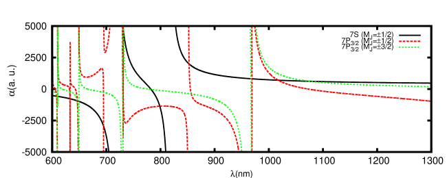
Figure 3: (Color online) Dynamic polarizabilities (in a.u.) for the $7S_{1/2}$ and $7P_{3/2}$ states of Fr in the wavelength range 600-1300 nm for linearly polarized light.

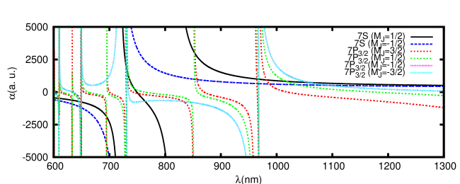
Figure 4: (Color online) Dynamic polarizabilities (in a.u.) for the $7S_{1/2}$ and $7P_{3/2}$ states of Fr in the wavelength range 600-1300 nm for left circularly polarized light(A=-1).

Table 2: Magic wavelengths ($\lambda_{\rm{magic}}$) (in nm) with corresponding polarizabilities ($\alpha_{n}(\omega)$) (in a.u.) for the $7S-7P_{1/2}$ transition in the Fr atom with linearly polarized light along with the resonant wavelengths ($\lambda_{\rm{res}}$) (in nm). Values that are found to be in discrepancy with $\lambda_{\rm{magic}}$ given in Ref. Dammalapati et al. (2016) are highlighted in bold fonts.

		Present		Ref. Dammalapati et al. (2016)
		$M_{j}$=$\pm 1/2$
Resonance	$\lambda_{\rm{res}}$	$\lambda_{\rm{magic}}$	$\alpha_{n}(\omega)$	$\lambda_{\rm{magic}}$
		621.48	-667	621.11
$7P_{1/2}-10S_{1/2}$	622.15
		646.05	-930	642.85
$7P_{1/2}-8D_{3/2}$	650.9
$7s_{1/2}-7P_{3/2}$	718.18
$7P_{1/2}-9S_{1/2}$	744.4
		745.6	2015	745.36
		771.03	520	797.75
$7S_{1/2}-7P_{1/2}$	817.17
$7P_{1/2}-7D_{3/2}$	832.87
		838.08	2933	871.62
$7P_{1/2}-8S_{1/2}$	1332.87
		1479.49	421

Table 3: Magic wavelengths ($\lambda_{\rm{magic}}$) (in nm) with corresponding polarizabilities ($\alpha_{n}(\omega)$) (in a.u.) for the $7S-7P_{1/2}$ transition in the Fr atom with circularly polarized light along with the resonant wavelengths ($\lambda_{\rm{res}}$) (in nm). Our values are compared with the corresponding $\lambda_{\rm{magic}}$ values given in Ref. Dammalapati et al. (2016).

		Transition: $7S(M_{J}=1/2)-7P_{1/2}$					Transition: $7S(M_{J}=-1/2)-7P_{1/2}$
		$M_{J}=1/2$			$M_{J}=-1/2$		$M_{J}=1/2$		$M_{J}=-1/2$
		Present		Ref. Dammalapati et al. (2016)
Resonance	$\lambda_{\rm{res}}$	$\lambda_{\rm{magic}}$	$\alpha_{n}(\omega)$	$\lambda_{\rm{magic}}$	$\lambda_{\rm{magic}}$	$\alpha_{n}(\omega)$	$\lambda_{\rm{magic}}$	$\alpha_{n}(\omega)$	$\lambda_{\rm{magic}}$	$\alpha_{n}(\omega)$
		620.10	-543				620.84	-774
$7P_{1/2}-10S_{1/2}$	622.15
		647.12	-741	640.25	643.24	-705	648.62	-1177	645.53	-1118
$7P_{1/2}-8D_{3/2}$	650.9
$7s_{1/2}-7P_{3/2}$	718.18
					739.24	662
$7P_{1/2}-9S_{1/2}$	744.4
									783.85	1741
$7S_{1/2}-7P_{1/2}$	817.17
$7P_{1/2}-7D_{3/2}$	832.87
		835.31	5459	1116.2	837.08	5017	844.72	1022	841.10	1045
$7P_{1/2}-8S_{1/2}$	1332.87

Table 4: Magic wavelengths ($\lambda_{\rm{magic}}$) (in nm) with corresponding polarizabilities ($\alpha_{n}(\omega)$) (in a.u.) for the $7S-7P_{3/2}$ transition in the Fr atom with linearly polarized light along with the resonant wavelengths ($\lambda_{\rm{res}}$) (in nm) and their comparison with the $\lambda_{\rm{magic}}$ values given in Ref. Dammalapati et al. (2016). Values showing large differences are shown in bold fonts.

Transition
$7S(M_{J}=\pm 1/2)-7P_{3/2}$		$M_{J}=\pm 1/2$			$M_{J}=\pm 3/2$
		Present		Ref. Dammalapati et al. (2016)	Present		Ref. Dammalapati et al. (2016)
Resonance	$\lambda_{\rm{res}}$	$\lambda_{\rm{magic}}$	$\alpha_{n}(\omega)$	$\lambda_{\rm{magic}}$	$\lambda_{\rm{magic}}$	$\alpha_{n}(\omega)$	$\lambda_{\rm{magic}}$
		600.89	-527	600.33
$7P_{3/2}-12S_{1/2}$	601.12
		608.15	-570	605.64	607.59	-566	606.66
$7P_{3/2}-10D_{5/2}$	609.70
		610.27	-584		610.18	-583	610.20
$7P_{3/2}-10D_{3/2}$	610.28
		632.83	-771	632.38
$7P_{3/2}-11S_{1/2}$	633.12
		646.49	-936	645.11	645.64	-924	645.95
$7P_{3/2}-9D_{5/2}$	648.60
		649.65	-983	649.65	649.50	-981	649.51
$7P_{3/2}-9D_{3/2}$	649.67
		694.92	-2943	694.67
$7P_{3/2}-10S_{1/2}$	695.09
$7S_{1/2}-7P_{3/2}$	718.18
$7P_{3/2}-8D_{5/2}$	728.79
		729.63	5469	730.51	729.77	5400	729.73
$7P_{3/2}-8D_{3/2}$	731.17
		731.21	4766	731.32	731.88	4512	731.77
		798.74	-1363	784.62	782.83	-39	783.35
$7S_{1/2}-7P_{1/2}$	817.17
$7P_{3/2}-9S_{1/2}$	851.28
		852.84	1990	853.93
$7P_{3/2}-7D_{5/2}$	960.71
		968.79	810	968.83	967.03	816	967.19
$7P_{3/2}-7D_{3/2}$	968.99
		1017.45	698	1266.3	1076.60	613	1117.7

Table 5: Magic wavelengths ($\lambda_{\rm{magic}}$) (in nm) with corresponding polarizabilities ($\alpha_{n}(\omega)$) (in a.u.) for the $7S(M_{J}=1/2)-7P_{3/2}$ transition in the Fr atom with left handed circularly polarized light ($A=-1$) along with the resonant wavelengths ($\lambda_{\rm{res}}$) (in nm). Our values are compared with the corresponding $\lambda_{\rm{magic}}$ values given in Ref. Dammalapati et al. (2016).

Transition: $7S(M_{J}=1/2)-7P_{3/2}$		$M_{J}=3/2$			$M_{J}=1/2$			$M_{J}=-1/2$		$M_{J}=-3/2$
		Present		Ref. Dammalapati et al. (2016)	Present		Ref. Dammalapati et al. (2016)
Resonance	$\lambda_{\rm{res}}$	$\lambda_{\rm{magic}}$	$\alpha_{n}(\omega)$	$\lambda_{\rm{magic}}$	$\lambda_{\rm{magic}}$	$\alpha_{n}(\omega)$	$\lambda_{\rm{magic}}$	$\lambda_{\rm{magic}}$	$\alpha_{n}(\omega)$	$\lambda_{\rm{magic}}$	$\alpha_{n}(\omega)$
		600.34	-446		600.87	-449
$7P_{3/2}-12S_{1/2}$	601.12
		608.86	-485	603.36	607.66	-479	605.99	607.32	-477	607.48	-478
$7P_{3/2}-10D_{5/2}$	609.70
		610.10	-491		610.16	-491		610.23	-491
$7P_{3/2}-10D_{3/2}$	610.28
		632.08	-619		632.76	-623
$7P_{3/2}-11S_{1/2}$	633.12
		647.41	-744	643.62	645.52	-726	645.60	645.11	-723	645.45	-726
$7P_{3/2}-9D_{5/2}$	648.60
		649.38	-763		649.47	-764	649.57	649.58	-765
$7P_{3/2}-9D_{3/2}$	649.67
		694.26	-1851		694.82	-1887
$7P_{3/2}-10S_{1/2}$	695.09
$7S_{1/2}-7P_{3/2}$	718.18
$7P_{3/2}-8D_{5/2}$	728.79
		729.34	2175	730.64	730.15	1960	729.76	730.36	1914	730.36	1914
$7P_{3/2}-8D_{3/2}$	731.17
		732.10	1557		734.63	1163	731.43	732.16	1547
		751.47	-124		744.27	282		763.69	-699	783.25	-1879
$7S_{1/2}-7P_{1/2}$	817.17
$7P_{3/2}-9S_{1/2}$	851.28
		853.60	2950		852.03	3063
$7P_{3/2}-7D_{5/2}$	960.71
		964.41	999		966.63	989		967.97	983
$7P_{3/2}-7D_{3/2}$	968.99
		982.05	925		1017.02	817	1395.3	1059.66	726	1062.67	721

Table 6: Magic wavelengths ($\lambda_{\rm{magic}}$) (in nm) with corresponding polarizabilities ($\alpha_{n}(\omega)$) (in a.u.) for the $7S(M_{J}=-1/2)-7P_{3/2}$ transition in the Fr atom with left handed circularly polarized light ($A=-1$) along with the resonant wavelengths ($\lambda_{\rm{res}}$) (in nm).

Transition: $7S(M_{J}=-1/2)-7P_{3/2}$		$M_{J}=3/2$		$M_{J}=1/2$		$M_{J}=-1/2$		$M_{J}=-3/2$
Resonance	$\lambda_{\rm{res}}$	$\lambda_{\rm{magic}}$	$\alpha_{n}(\omega)$	$\lambda_{\rm{magic}}$	$\alpha_{n}(\omega)$	$\lambda_{\rm{magic}}$	$\alpha_{n}(\omega)$	$\lambda_{\rm{magic}}$	$\alpha_{n}(\omega)$
		600.59	-602	600.95	-605
$7P_{3/2}-12S_{1/2}$	601.12
		609.16	-668	608.30	-661	607.86	-657	607.82	-657
$7P_{3/2}-10D_{5/2}$	609.70
		610.13	-676	610.17	-676	610.23	-677
$7P_{3/2}-10D_{3/2}$	610.28
		632.50	-913	632.91	-918
$7P_{3/2}-11S_{1/2}$	633.12
		647.96	-1165	646.81	-1143	646.17	-1131	646.08	-1129
$7P_{3/2}-9D_{5/2}$	648.60
		649.45	-1196	649.50	-1197	649.59	-1199
$7P_{3/2}-9D_{3/2}$	649.67
		694.73	-3959	694.97	-4002
$7P_{3/2}-10S_{1/2}$	695.09
$7S_{1/2}-7P_{3/2}$	718.18
$7P_{3/2}-8D_{5/2}$	728.79
		728.95	9382	729.28	9113	729.57	8890	729.72	8777
$7P_{3/2}-8D_{3/2}$	731.17
		731.33	7727	731.43	7669	731.35	7718
$7S_{1/2}-7P_{1/2}$	817.17
$7P_{3/2}-9S_{1/2}$	851.28
		857.06	954	853.19	974
$7P_{3/2}-7D_{5/2}$	960.71
		964.69	648	966.73	645	968.01	643
$7P_{3/2}-7D_{3/2}$	968.99
		987.2	616	1037.18	560	1092.01	517	1083.72	522

IV Results and Discussion

Accurate determination of $\alpha_{n}$ is very crucial in predicting $\rm\lambda_{magic}$ precisely. In order to reduce the uncertainties in estimation of “Main($\alpha_{n,v}^{(i)}$)” contributions of the ground and the first two excited $7P_{1/2,3/2}$ states of the considered Fr atom, we use the experimentally driven precise values of E1 matrix elements for the $7S-7P_{1/2}$ and $7S-7P_{3/2}$ transitions, which are extracted from the lifetime measurements of the $7P_{1/2,3/2}$ states Simsarian et al. (1998) and determine as many as E1 matrix elements of the transitions involving the low-lying states up to $11P$, $11S$ and $10D$ using the CCSD(T) method. Further, we improve the results by using excitation energies from the measurements as listed in the National Institute of Science and Technology (NIST) database Kramida et al. (2012). In order to demonstrate role of various contributions to $\alpha_{n}$, we give individual contributions from different E1 matrix elements to “Main($\alpha_{n,v}^{(i)}$)”, “Tail($\alpha_{n,v}^{(i)}$)”, $\alpha_{n,c}^{(i)}$ and $\alpha_{n,cv}^{(i)}$ (where $i=0,2$) explicitly along with the net results in the evaluation of static polarizabilities ($\omega=0$) in atomic unit (a.u.) in Table 1. Moreover, we verify validity of these results by comparing with the previously reported other precise calculations in Refs. Derevianko et al. (1999); Lim et al. (2005); Wijngaarden and Xia (1999) since the experimental data for these results is not available.

As seen in Table 1, our calculated $\alpha_{n}(0)$ value of 316.8 a.u. for the ground state of Fr atom is in agreement with the $\alpha_{n}(0)$ value of 317.8(2.4) a.u., which is calculated by Derevianko et al. using a relativistic all order method Derevianko et al. (1999). Lim et al. had also calculated the static polarizability for the ground state as 315.2 a.u. using another RCC method in finite gradient approach considering Douglas-Kroll Hamiltonian Lim et al. (2005). Our result matches well with this value as well, indicating validity of our calculation. The value of $\alpha_{n}(0)$ for the $7P_{1/2}$ state is estimated to be 1225 a.u., which agrees with the one given by Wijngaarden et al. as 1106 a.u. Wijngaarden and Xia (1999). Similarly, our calculated values for the static scalar and tensor polarizabilities of the $7P_{3/2}$ state in Fr are obtained as 2304 a.u. and $-467$ a.u., respectively. These results are again in reasonable agreement with the respective values given by Wijngaarden et al. as 2102 a.u. and $-402.7$ a.u. respectively Wijngaarden and Xia (1999). The reason for minor differences between our values and those obtained by Wijngaarden et al. could be because of the fact that the later calculations were carried out in a semi-empirical approach with the Coulomb approximation, while our calculations are more rigorous. Nevertheless, reasonable agreement between our calculations and the values reported by other theoretical calculations using a variety of many-body methods Derevianko et al. (1999); Lim et al. (2005); Wijngaarden and Xia (1999) ascertain that our static values of $\alpha_{n}$ are reliable enough; in fact, we estimate about 1% accuracy in our static polarizability values. Correspondingly, we expect that the dynamic polarizabilities evaluated in our calculations are also accurate enough to determine $\lambda_{\rm{magic}}$ for the $7S_{1/2}-7P_{1/2,3/2}$ transitions in Fr.

Now to fathom about the accuracies in the estimated $\alpha_{n}$’s of the considered states in Fr by Dammalapati et al. Dammalapati et al. (2016), we consider the E1 matrix elements referred in their paper and use the experimental energies to reproduce the corresponding static polarizability values. As discussed in Sec. II(A) and II(B) of Ref. Dammalapati et al. (2016), they take into account the E1 matrix elements of the $7S-nP$ transitions with $n=7-20$ from Ref. Sansonetti (2007) to evaluate dynamic $\alpha_{n}$ of the ground state. Similarly, they consider E1 matrix elements of the $7P-nS$ transitions for $n=9-20$ and $7P-nD$ transitions for $n=7-20$ states to evaluate $\alpha$ of the $7P_{1/2,3/2}$ states. Using the above referred data we were also able to reproduce plots given in Figs. 1-3 of Ref. Dammalapati et al. (2016). The $\alpha_{n}(0)$ values obtained from these quoted matrix elements are given in Table 1. These values are 289.8 a.u., 57.23 a.u. and 98.57 a.u. for the scalar polarizabilities of the ground, $7P_{1/2}$ and $7P_{3/2}$ states respectively, while it is equal to 63.23 a.u. for the tensor polarizability of the $7P_{3/2}$ state. Compared to other calculations and our results, the reproduced ground state values differ slightly and mainly due to the extra core correlation effect taken into account in our calculation. In contrast, we find huge differences in the $\alpha_{n}(0)$ values of the $7P$ excited states. In accordance with the explicit contributions given in Table 1, we observe that this discrepancy is mainly due to omission of the E1 matrix element contributions from the $7P_{1/2}-6D_{3/2}$ and $7P_{3/2}-6D_{5/2}$ transitions, which alone contribute more than 60% to the total polarizabilities of the $7P_{1/2}$ and $7P_{3/2}$ states. This obviously implies that $\alpha_{n}$ used by Dammalapati et al. are not reliable enough for determining $\lambda_{\rm{magic}}$ precisely.

In pursuance of demonstrating $\rm\lambda_{magic}$ for the $7S-7P_{1/2,3/2}$ transitions in Fr, we plot the dynamic $\alpha_{n}$ values of the $7S$, $7P_{1/2}$ and $7P_{3/2}$ states in Figs. 1, 2, 3 and 4 for both linearly and circularly polarized light separately. The wavelengths at which this intersection takes place are identified as $\lambda_{\rm{magic}}$ and are listed in Tables 2, 3, 4, 5 and 6. As discussed in Ref. Arora et al. (2007) the occurrence of $\lambda_{\rm{magic}}$ can be predicted between the resonant wavelengths $\lambda_{\rm{res}}$ which has also been listed in these tables along with the corresponding resonant transition. $\rm\lambda_{magic}$ are tabulated in rows lying between two resonances to identify the placements of $\lambda_{\rm{magic}}$ clearly between two $\lambda_{\rm{res}}$. Below we discuss these results for the $7S-7P_{1/2}$ and $7S-7P_{3/2}$ transitions separately for both linearly and circularly polarized light and highlight the discrepancies in our results from the results presented in Ref. (Dammalapati et al., 2016).

IV.1 $\rm\lambda_{magic}$ for the $7S-7P_{1/2}$ transition

A total of six $\rm\lambda_{magic}$ for the $7S-7P_{1/2}$ transition using linearly polarized light are listed in Table 2 in the wavelength range 600-1500 nm. Major differences found between our results from the values presented in Ref. Dammalapati et al. (2016) are marked in bold font. A $\rm\lambda_{magic}$ reported at 642.85 nm in Ref. (Dammalapati et al., 2016) is instead of found to be at 646.05 nm. Our analysis suggests this discrepancy is mainly due to different E1 amplitude of the $7P_{1/2}-8D_{3/2}$ transition obtained by the CCSD(T) method in the present work as compared to the one obtained using the HFR method in Ref. Dammalapati et al. (2016). In near infrared region (i.e. 700-1200 nm), two out of three $\rm\lambda_{magic}$ are identified at different wavelengths using our method as compared to $\rm\lambda_{magic}$ reported by Dammalapati et al.. This disagreement is mainly due to inclusion of the E1 amplitude of the $7S-7P_{1/2}$ transition in the present calculation of $7P_{1/2}$ polarizability which play crucial role in this region. As a consequence, we find a $\rm\lambda_{magic}$ at 771.03 nm supporting a red detuned trapping scheme, which is evident from the positive sign of the polarizability values at this wavelength as shown in Fig. 1 and quoted in Table 2. Instead this was reported at 797.75 by Dammalapati et al. and was seen supporting a blue detuned trap in Fig. 3(a) of Ref. Dammalapati et al. (2016), since the corresponding light shift value had positive sign at this wavelength. Similarly, the $\rm\lambda_{magic}$ for the $7S-7P_{1/2}$ transition using circularly polarized light are tabulated in Table 3 and graphically presented in Fig. 2. In the present work, we determine $\rm\lambda_{magic}$s for left circularly polarization using $A=-1$ considering all possible positive and negative $M_{J}$ sublevels of the states participating in the transition. Note that $\rm\lambda_{magic}$ for the right circularly polarized light of a transition with a given $M_{J}$ are equal to left circularly polarized light with opposite sign of $M_{J}$. From Table 3, we find large differences between $\rm\lambda_{magic}$ reported in Ref. Dammalapati et al. (2016) and those obtained by us.

IV.2 $\rm\lambda_{magic}$ for the $7S-7P_{3/2}$ transition

The $\rm\lambda_{magic}$ for the $7S-7P_{3/2}$ transition are identified from the crossings of the dynamic polarizabilities of the $7S$ and $7P_{3/2}$ states as shown from their plotting in Figs. 3 and 4 for both linearly and circularly polarized light respectively. These values are presented separately in Table 4 for the $7S-7P_{3/2}$ transition using linearly polarized light while they are given in Tables 5 and 6 for the $7S(M_{J}=1/2)-7P_{3/2}$ and $7S(M_{J}=-1/2)-7P_{3/2}$ transitions, respectively, using circularly polarized light. At least four discrepancies among $\rm\lambda_{magic}$ are found in comparison to the values reported in Ref. Dammalapati et al. (2016) and are highlighted in bold fonts in the above tables. The first disagreement is in the $\rm\lambda_{magic}$ value reported in this work at 608.15 nm in the vicinity of the $7P_{3/2}-10D_{5/2}$ transition, but was identified at 605.64 nm in Ref. Dammalapati et al. (2016). The reason for this disagreement is primarily due to the difference in the E1 matrix element for the $7P_{3/2}-10D_{5/2}$ transition used in both the works, which contributes significantly around this wavelength. As shown in Table 1, the E1 matrix element for the $7P_{3/2}-10D_{5/2}$ transition obtained by the CCSD(T) method is 1.27 a.u., whereas, the value used by Dammalapati et al. was 1.55 a.u.. From Table 4, it is also evident that we are able to identify one $\rm\lambda_{magic}$ for the $7S-7P_{3/2}(M_{J}=\pm 1/2)$ transition at 610.27 nm, there was no corresponding value was found in Ref. Dammalapati et al. (2016). Moreover, $\rm\lambda_{magic}$ for the above transition reported at 784.62 nm by Dammalapati et al. in Fig. 2 of Ref. Dammalapati et al. (2016) is close to the tune-out wavelength (wavelength at which the ac polarizability of the ground state becomes zero). As seen in Table 4, the value of ac polarizability at the corresponding $\rm\lambda_{magic}$ at 798.74 nm comes out to be a large negative value in this work. Hence, the trap at this $\rm\lambda_{magic}$ indicate to support a strong blue detuned trap as compared to a shallow blue detuned trap portrayed in Ref.  Dammalapati et al. (2016). Similarly, our calculated and their reported $\rm\lambda_{magic}$ after the resonant transition $7P_{3/2}-7D_{3/2}$ (beyond 968.99 nm) are completely different. This can be attributed to the fact that the resonant transitions which appear after 968.99 nm (i.e. $7P_{3/2}-8S_{1/2}$, $7P_{3/2}-6D_{5/2}$ and $7P_{3/2}-6D_{3/2}$ transitions) have not been taken into account by Dammalapati et al. in their calculation of the $7P_{3/2}$ state polarizabilities. Furthermore, we have listed $\rm\lambda_{magic}$ for the $7S(M_{J}=1/2)-7P_{3/2}$ and $7S(M_{J}=-1/2)-7P_{3/2}$ transitions using circularly polarized light in Tables 5 and 6. In this case too, we find more number of $\rm\lambda_{magic}$ and the ones reported by Dammalapati et al. do not agree with our values at most of the places.

V Conclusion

In summary, we present a list of recommended magic wavelengths for the $7S-7P_{1/2,3/2}$ transitions of the Fr atom considering both linearly and circularly polarized light, which will be very useful to trap Fr atoms at these wavelengths for high precision experiments. We have calculated dynamic electric dipole polarizabilities of the ground and $7P_{1/2,3/2}$ states of Fr by combining matrix elements calculated using the precisely measured lifetimes of the $7P_{1/2,3/2}$ states and performing calculations of higher excited states using a relativistic coupled-cluster method. Reliability of these results are verified by comparing the static dipole polarizability values with the other available theoretical results. Since experimental results of these quantities are not available, our calculations will serve as bench mark values for the future measurements. The magic wavelengths for these transitions were investigated earlier using electric dipole matrix elements from literature, but omitting many dominant contributions such as core correlation contribution and some very important E1 transitions. We present the revised values of the magic wavelengths of the above D-lines for both linearly and circularly polarized light in the optical region taking into account all the omitted contributions. We even highlight the discrepancy in the prediction of different kind of trap to be used at some magic wavelengths in the present work and as interpreted from the previous study. These magic wavelengths will be of immense interest to the experimentalists to carry out cold atom experiments and investigating many fundamental physics using Fr atoms.

References

- Sakemi et al. (2011) Y. Sakemi, K. Harada, T. Hayamizu, M. Itoh, H. Kawamura, S. Liu, H. S. Nataraj, A. Oikawa, M. Saito, T. Sato, et al., Journal of Physics: Conference Series 302, 012051 (2011).
- Inoue et al. (2015) T. Inoue et al., Hyperfine Interactions 231, 157 (2015).
- Mukherjee and Pal (1989) D. Mukherjee and S. Pal, Adv. Quant. Chem. 20, 281 (1989).
- Stancari et al. (2007) G. Stancari, S. N. Atutov, R. Calabrese, L. Corradi, A. Dainelli, C. de Mauro, A. Khanbekyan, E. Mariotti, P. Minguzzi, L. Moi, et al., Eur. Phys. J. Special Topics 150, 389 (2007).
- Sahoo (2010) B. K. Sahoo, J. Phys. B 43, 085005 (2010).
- Gomez et al. (2007) E. Gomez, S. Aubin, G. D. Sprouse, L. A. Orozco, and D. P. DeMille, Phys. Rev. A 75, 033418 (2007).
- Sahoo et al. (2016) B. K. Sahoo, T. Aoki, B. P. Das, and Y. Sakemi, Phys. Rev. A 93, 032520 (2016).
- Sahoo et al. (2015) B. K. Sahoo, D. K. Nandy, B. P. Das, and Y. Sakemi, Phys. Rev. A 91, 042507 (2015).
- Sahoo and Das (2015) B. K. Sahoo and B. P. Das, Phys.Rev. A 92, 052511 (2015).
- Sahoo (2015) B. K. Sahoo, Phys. Rev. A 92, 052506 (2015).
- Simsarian et al. (1998) J. E. Simsarian, L. A. Orozco, G. D. Sprouse, and W. Z. Zhao, Phys. Rev. A 57, 4 (1998).
- Atutov et al. (2015) S. N. Atutov, R. Calabrese, L. Corradi, and L. Tomasseti, Proceedings of SPIE - The International Society for Optical Engineering 92, 052506 (2015).
- Dammalapati et al. (2016) U. Dammalapati, K. Harada, and Y. Sakemi, Phys. Rev. A 93, 043407 (2016).
- Phillips (1998) W. D. Phillips, Rev. Mod. Phys. 70, 721 (1998).
- Simsarian et al. (1996) J. E. Simsarian, A. Ghosh, G. Gwinner, L. A. Orozco, G. D. Sprouse, and P. A. Voytas, Phys. Rev. Lett. 76, 19 (1996).
- Katori et al. (1999) H. Katori, T. Ido, and M. Kuwata-Gonokami, J. Phys. Soc. Jpn. 668 668, 2479 (1999).
- McKeever et al. (2003) J. McKeever, J. R. Buck, A. D. Boozer, A. Kuzmich, H.-C. Nagerl, D. M. Stamper-Kurn, and H. J. Kimble, Phys. Rev. Lett. 90, 133602 (2003).
- Arora et al. (2007) B. Arora, M. S. Safronova, and C. W. Clark, Phys. Rev. A 76, 052509 (2007).
- Arora and Sahoo (2012) B. Arora and B. K. Sahoo, Phys. Rev. A 86, 033416 (2012).
- Sahoo and Arora (2013) B. K. Sahoo and B. Arora, Phys. Rev. A 87, 023402 (2013).
- Singh et al. (2016a) S. Singh, K. Kaur, B. K. Sahoo, and B. Arora, J. Phys. B: At. Mol. Opt. Phys. 49, 145005 (2016a).
- Singh et al. (2016b) S. Singh, B. K. Sahoo, and B. Arora, Phys. Rev. A 93, 06342 (2016b).
- Sansonetti (2007) J. E. Sansonetti, J. Phys. Chem. Ref. Data 36, 497 (2007).
- Biemont et al. (1998) E. Biemont, P. Quinet, and V. V. Renterghem, J. Phys. B: At. Mol. Opt. Phys. 31, 5301 (1998).
- Derevianko et al. (1999) A. Derevianko, W. R. Johnson, M. S. Safronova, and J. F. Babb, Phys. Rev. Lett. 82, 3589 (1999).
- Wijngaarden and Xia (1999) W. A. V. Wijngaarden and J. Xia, J. Quant. Spectrosc. Radiat. Transfer 61, 557 (1999).
- Lim et al. (2005) I. Lim, P. Schwerdtfeger, B. Metz, and H. Stoll, J. Chem. Phys. 122, 104103 (2005).
- Bonin and Kresin (1997) K. D. Bonin and V. V. Kresin, Electric-dipole Polarizabilities of Atoms, Molecules and Clusters (World Scientific, Singapore, 1997).
- Manakov et al. (1986) N. L. Manakov, V. D. Ovsiannikov, and L. P. Rapoport, Phys. Rep. 141, 319 (1986).
- Beloy (2009) K. Beloy, Theory of the ac stark effect on the atomic hyperfine structure and applications to microwave atomic clocks (2009), ph.D. thesis, University of Nevada, Reno, USA.
- Arora et al. (2012) B. Arora, D. K. Nandy, and B. K. Sahoo, Phys. Rev. A 85, 012506 (2012).
- Kaur et al. (2015) J. Kaur, D. K. Nandy, B. Arora, and B. K. Sahoo, Phys. Rev. A 91, 012705 (2015).
- Singh and Sahoo (2014) Y. Singh and B. K. Sahoo, Phys. Rev. A 90, 022511 (2014).
- Kramida et al. (2012) A. Kramida, Y. Ralchenko, J. Reader, and N. A. T. (2012), Nist atomic spectra database (2012), (version 5). [Online]. Available: http://physics.nist.gov/asd [2012, December 12]. National Institute of Standards and Technology, Gaithersburg, MD.