Combined effect of horizontal magnetic field and vorticity on Rayleigh -Taylor instability

Abstract

In this research, the height, curvature and velocity of the bubble tip in Rayleigh-Taylor instability at arbitrary Atwood number with horizontal magnetic field are investigated. To support the earlier simulation and experimental results, the vorticity generation inside the bubble is introduced. It is found that, in early nonlinear stage, the temporal evolution of the bubble tip parameters depend essentially on the strength and initial perturbation of the magnetic field, although the asymptotic nature coincides with the non magnetic case. The model proposed here agrees with the previous linear, nonlinear and simulation observations.

I INTRODUCTION

The Rayleigh-Taylor Instability occurs when a lighter density fluid pushes the heavier one against the gravitational force field. This instability appears in many physical and astrophysical situations, such as Inertial Confinement Fusion, where the magnetic field provides a stabilizing effect of the two fluid instability[1], overturn of the outer portion of the collapsed core of massive stars, etc. In the linear regime, the perturbation grows exponentially with the growth rate $\sqrt{Akg}$, where $A=\frac{\rho_{h}-\rho_{l}}{\rho_{h}+\rho_{l}}$ is the Atwood number, $\rho_{h}$ and $\rho_{l}$ are the densities of heavier and lighter fluid, respectively, $k$ is the perturbation wave number and $g$ is the interfacial acceleration [2]. In the nonlinear stage, the interface can be divided into the bubble of the lighter fluid rising into the heavier fluid, and spike of the heavier fluid penetrating into the lighter fluid. There are several methods for describing the nonlinear effect on this instability. Among them, Layzer’s [3] describes a formulation where the interface near the tip of the bubble is approximated by a parabola and determined the position, curvature and velocity of the bubble tip. Extending this model, Goncharov [4] derived the asymptotic velocity of the bubble tip, which is $\sqrt{\frac{2A}{1+A}\frac{g}{3k}}$. However, the observed simulation and experimental results [5, 6, 7] indicate that nonlinear theory correctly captures the bubble behavior in the early nonlinear phase, but fails in the highly nonlinear stage. Betti and Sanz [6] shows that this occurs due to vorticity accretion inside the bubble and the velocity of the bubble tip is slightly higher than the classical value obtained by Goncharov [4].

In an Inertial Confinement Fusion situation or in the astrophysical situation the fluid may be ionized or may get ionized through laser irradiation in laboratory condition. In this case the study of magnetic field effect on Rayleigh-Taylor instability is needed. Under the linear theory, the influence of magnetic field on Rayleigh-Taylor instability has been studied in detail by Chandrasekhar [2]. He observed that, when the magnetic field is parallel to the interface separating of two fluids, the growth rate of the Rayleigh-Taylor instability is unaffected by magnetic field. However, using Layzer’s model, Gupta et. al[1] pointed that the parallel magnetic field becomes a stabilizing factor of the instability.

The asymptotic growth, curvature and growth rate of the bubble tip in Rayleigh-Taylor instability, which is one of the main factors in Inertial Confinement Fusion or in laboratory experiments, have been discussed by analytical and numerical approaches. In the presence of magnetic field, the dynamics of the bubble tip has been analyzed by considering the vorticity accumulation inside the bubble. The magnetic field is assumed to be parallel to the plane of the two fluid interface and acts in a direction perpendicular to the wave vector. The basic model is based on the Layzer’s theory.

The structure of the paper is as follows. Section II describes the kinematical and dynamical boundary conditions for the temporal evolution of the bubble tip in Rayleigh-Taylor instability for incompressible, inviscid fluids. Here the heavier fluid is assumed to be irrotational where the lower one is rotational. The results and discussions are presented in Section III.

II Basic Equations and Boundary Conditions

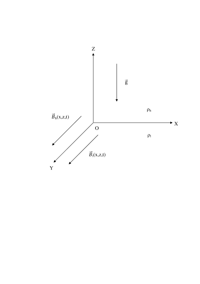
Figure 1: Schematic diagram of the model.

We suppose that a fluid of density $\rho_{h}$ lies in the region $z>0$ and that a second fluid of density $\rho_{l}$ lies in the region $z<0$. The system is subject to a uniform acceleration $g$ in the negative direction of $z$ axis (see Fig.1). The magnetic field is taken along the direction of $y$ axis, i.e, parallel to the surface of separation.

$$\vec{B}=\left\{\begin{array}[]{lr}\widehat{y}B_{h}(x,z,t)&:z>0\\ \widehat{y}B_{l}(x,z,t)&:z<0\end{array}\right.$$ (3)

According to the chosen magnetic field $\vec{\nabla}.\vec{B}=0$ everywhere.

Here we are considering two dimensional problem. Therefore we approximate the perturbed interface by a parabola, given by

$$z=\eta(x,t)=\eta_{0}(t)+\eta_{2}(t)x^{2}$$ (4)

where, for a bubble, $\eta_{0}(t)>0$ and $\eta_{2}(t)<0$.

The kinematical boundary conditions satisfied by the interfacial surface $z=\eta(x,t)$ are

$$\frac{\partial\eta}{\partial t}+v_{hx}\frac{\partial\eta}{\partial x}=v_{hy}$$ (5)

$$\frac{\partial\eta}{\partial x}(v_{hx}-v_{lx})=v_{hy}-v_{ly}$$ (6)

where $(v_{h,l})_{x,y}$ are the velocity components of the heavier and lighter fluids, respectively.

The fluid motion is governed by the ideal magnetohydrodynamic equations

$$\rho[\frac{\partial\vec{v}}{\partial t}+(\vec{v}\cdot\vec{\nabla})\vec{v}]+\vec{\nabla}(p+g\rho z)=\frac{1}{\mu}(\vec{\nabla}\times\vec{B})\times\vec{B}=\frac{1}{\mu}(\vec{B}\cdot\vec{\nabla})\vec{B}-\frac{1}{2\mu}\vec{\nabla}(B^{2})=-\frac{1}{2\mu}\vec{\nabla}(B^{2})$$ (7)

[$\frac{1}{\mu}(\vec{B}\cdot\vec{\nabla})\vec{B}=0$, as $\vec{B}(x,z,t)$ is taken along the $y$ axis]

$$\frac{\partial\vec{B}}{\partial t}=\vec{\nabla}\times(\vec{v}\times\vec{B})$$ (8)

According to Layzer’s model [3, 8], the velocity potential describing the irrotational motion for the heavier fluid is assumed to be given by

$$\phi_{h}(x,z,t)=a(t)\cos(kx)e^{-k(z-\eta_{0}(t))}$$ (9)

with $\vec{v_{h}}=-\vec{\nabla}\phi_{h}$.

Since $\vec{\nabla}\cdot\vec{v_{h}}=0$, the equation of motion of the upper incompressible fluid leads to the following integral [7]:

$$\rho_{h}[-\frac{\partial\phi_{h}}{\partial t}+\frac{1}{2}(\vec{\nabla}\phi_{h})^{2}+gz]+p_{h}+\frac{1}{2\mu_{h}}B_{h}^{2}=f_{h}(t)$$ (10)

For the lighter fluid the motion inside the bubble is assumed rotational [6] with vorticity $\vec{\omega}=(\frac{\partial v_{lz}}{\partial x}-\frac{\partial v_{lx}}{\partial z}){\hat{y}}$. The motion is described by the stream function $\Psi(x,y,t)$, given by

$$\Psi(x,z,t)=b_{0}(t)x+[b_{1}(t)e^{k(z-\eta_{0})}+\omega_{0}(t)/k^{2}]\sin{(kx)}$$ (11)

with $v_{lx}=-\frac{\partial\Psi}{\partial z}$ and $v_{lz}=\frac{\partial\Psi}{\partial x}$.

Hence

$$\nabla^{2}\Psi=-\omega$$ (12)

Let $\chi(x,z,t)$ be a function such that

$$\nabla^{2}\chi=-\omega$$ (13)

Hence $(\Psi-\chi)$ is a harmonic function as $\nabla^{2}(\Psi-\chi)=0$. Let $\Phi(x,z,t)$ be its conjugate function

$$\frac{\partial\Phi}{\partial x}=\frac{\partial\Psi}{\partial z}-\frac{\partial\chi}{\partial z}$$

$$\frac{\partial\Phi}{\partial z}=-\frac{\partial\Psi}{\partial x}+\frac{\partial\chi}{\partial x}$$ (14)

Thus the velocity components of the lighter fluid are

$$v_{lx}=-\frac{\partial\Psi}{\partial z}=-\frac{\partial\Phi}{\partial x}-\frac{\partial\chi}{\partial z}$$

$$v_{lz}=\frac{\partial\Psi}{\partial x}=-\frac{\partial\Phi}{\partial z}+\frac{\partial\chi}{\partial x}$$ (15)

Using Eqs.(10)-(13), the first integral of the equation of motion of the lighter fluid is given by

$$\rho_{l}[-\frac{\partial\Phi}{\partial t}+\frac{1}{2}(\vec{v}_{l}){{}^{2}}-\omega\Psi+gz]+\int\rho_{l}[(\Psi\frac{\partial\omega}{\partial z}-\frac{\partial\dot{\chi}}{\partial z})dx+(\Psi\frac{\partial\omega}{\partial x}+\frac{\partial\dot{\chi}}{\partial x})dz]+p_{l}+\frac{1}{2\mu_{l}}B_{l}^{2}=f_{l}(t)$$ (16)

Here we set

$$\chi(x,z,t)=\omega_{0}(t)\sin{(kx)}/k^{2}$$ (17)

Therefore Eq.(13) gives

$$\Phi(x,z,t)=-b_{0}(t)y+b_{1}(t)\cos{(kx)}e^{k(z-\eta_{0})}$$ (18)

From Eqs.(8) and (14), we obtain our dynamical boundary condition:

$$\rho_{h}[-\frac{\partial\phi_{h}}{\partial t}+\frac{1}{2}(\vec{\nabla}\phi_{h})^{2}+gz]-\rho_{l}[-\frac{\partial\Phi}{\partial t}+\frac{1}{2}(\vec{\nabla}\Phi){{}^{2}}-\omega\Psi+gz]-\int\rho_{l}[(\Psi\frac{\partial\omega}{\partial z}-\frac{\partial\dot{\chi}}{\partial z})dx$$

$$+(\Psi\frac{\partial\omega}{\partial x}+\frac{\partial\dot{\chi}}{\partial x})dz]+(p_{h}-p_{l})+(\frac{1}{2\mu_{h}}B_{h}^{2}-\frac{1}{2\mu_{l}}B_{l}^{2})=f_{h}(t)-f_{l}(t)$$ (19)

satisfied at the interface $z=\eta(x,t)$.

Now we turn to our magnetic field equations. In virtue of Eqs. (1) and (6) the magnetic fields are assumed to be

$$B_{h}(x,z,t)=\beta_{h0}(t)+\beta_{h1}(t)e^{-k(z-\eta_{0})}\cos{(kx)}$$ (20)

$$B_{l}(x,z,t)=\beta_{l0}(t)+\beta_{l1}(t)e^{k(z-\eta_{0})}\cos{(kx)}$$ (21)

Substituting $\eta(x,t)$, $v_{hx}$, $v_{hz}$, $v_{lx}$ and $v_{lz}$ in Eqs. (3) and (4), and expanding in powers of the transverse coordinate $x$ and neglecting terms $O(x^{i})$ ($i\geq 3$), we obtain the following equations [8]

$$\frac{d\xi_{1}}{d\tau}=\xi_{3}$$ (22)

$$\frac{d\xi_{2}}{d\tau}=-\frac{1}{2}(6\xi_{2}+1)\xi_{3}$$ (23)

$$\frac{kb_{0}}{\sqrt{kg}}=\frac{6\xi_{2}(2\xi_{3}-\Omega)}{(6\xi_{2}-1)}$$ (24)

$$\frac{k^{2}b_{1}}{\sqrt{kg}}=-\frac{(6\xi_{2}+1)\xi_{3}-\Omega}{(6\xi_{2}-1)}$$ (25)

where $\xi_{1}=k\eta_{0}$, $\xi_{2}=\frac{\eta_{2}}{k}$ and $\xi_{3}=\frac{k^{2}a}{\sqrt{kg}}$ are the nondimensionalized bubble height, curvature and velocity respectively, $\tau=t\sqrt{kg}$ is the nondimensionalized time and $\Omega=\frac{\omega_{0}}{\sqrt{kg}}$ is the nondimensionalized vorticity.

Next substituting for the velocity components $v_{hx}$, $v_{hz}$, $v_{lx}$, $v_{lz}$ and $B_{h}(x,z,t)$, $B_{l}(x,z,t)$ in the Eq.(6) and equating coefficients of $x^{i}$ for $i=0$ and $2$ we obtain the following four equations

$$\dot{\beta}_{h0}+\dot{\beta}_{h1}=0\hskip 5.0pt\mbox{i.e, }\beta_{h0}+\beta_{h1}=B_{h0}\hskip 5.0pt\mbox{(say)}$$ (26)

$$\frac{d\xi_{4}}{d\tau}=\xi_{3}\xi_{4}\frac{2\xi_{2}-1}{2\xi_{2}+1}$$ (27)

and

$$\dot{\beta}_{l0}+\dot{\beta}_{l1}=0\hskip 5.0pt\mbox{i.e, }\beta_{l0}+\beta_{l1}=B_{l0}\hskip 5.0pt\mbox{(say)}$$ (28)

$$\frac{d\xi_{5}}{d\tau}=\xi_{5}\frac{\xi_{3}(2\xi_{2}+1)(6\xi_{2}+1)+2\Omega(2\xi_{2}-1)}{(2\xi_{2}-1)(6\xi_{2}-1)}$$ (29)

where $\xi_{4}=\frac{\beta_{h1}}{B_{h0}}$ and $\xi_{5}=\frac{\beta_{l1}}{B_{l0}}$.

Again the fluid pressures together with the magnetic pressures on both sides of the interface are equal [1], i.e.,

$$p_{h}+\frac{B_{h0}^{2}}{2\mu_{h}}=p_{l}+\frac{B_{l0}^{2}}{2\mu_{l}}$$ (30)

Using Eq.(28) in Eq.(17), the coefficient of $x^{2}$ of Eq .(17) gives the following equation for $\xi_{3}$.

$$\frac{d\xi_{3}}{d\tau}=\frac{1}{D(\xi_{2},r)}[-N(\xi_{2},r)\frac{\xi_{3}^{2}}{(6\xi_{2}-1)}+2(r-1)(6\xi_{2}-1)\xi_{2}+\frac{\Omega^{2}-5(6\xi_{2}+1)\Omega\xi_{3}}{(1-6\xi_{2})}+\dot{\Omega}]$$

$$-\frac{6\xi_{2}-1}{D(\xi_{2},r)}[rV_{h}^{2}\xi_{4}(2\xi_{2}+1)+V_{l}^{2}\xi_{5}(2\xi_{2}-1)]$$ (31)

where

$$N(\xi_{2},r)=36(1-r)\xi_{2}^{2}+12(4+r)\xi_{2}+(7-r)$$ (32)

$$D(\xi_{2},r)=12(1-r)\xi_{2}^{2}+4(1-r)\xi_{2}+(r+1)$$ (33)

$r=\frac{\rho_{h}}{\rho_{l}}$ and $V_{h(l)}=\frac{kB_{h0(l0)}^{2}}{\rho_{h(l)}\mu_{h(l)}g}$ is the normalized Alfven velocity.

Thus the magnetic field affected Rayleigh - Taylor instability induced growth of the bubble tip is determined by the parameters $\xi_{1}(t)$, $\xi_{2}(t)$, $\xi_{3}(t)$ as also the magnetic induction perturbation $\xi_{4}(t)$ and $\xi_{5}(t)$ given by Eqs. (20), (21), (29), (25) and (27).

III Results and Discussions

The system of equations given by Eqs. (20), (21), (29), (25) and (27) for the fluid parameters show that the complete understanding of the Rayleigh-Taylor instability is not possible without knowing the dependence of the vorticity $\Omega(\tau)$ on $\tau$. According to the simulation results obtained by Snaz and Betti [6], we chose the $\Omega(\tau)$ in the following form so that the time dependence of $\Omega(\tau)$ has approximate qualitative agrement with the simulation results.

$$\Omega(\tau)=\frac{\Omega_{c}}{1+2\tanh(\tau_{0})}[\tanh(\tau_{0})(1+\tanh(\tau))+\tanh(\tau-\tau_{0})]$$ (34)

Clearly $\Omega(\tau)$ increases from $0$ and tends to an asymptotic value $\Omega_{c}$ as $\tau\rightarrow\infty$. The constants $\tau_{0}$ and $\Omega_{c}$ are adjusted accordingly to Ref.[6]. The plot for $\Omega(\tau)$ is shown in Fig.2. It is clear from the figure that the $\tau_{0}=8$ and $\Omega_{c}=2$ give a good approximation of the simulation results.

To integrate the system of equations numerically, it is necessary to know the initial value of the parameters. The initial interface is assumed to be $z=\eta_{0}(t=0)\cos(kx)$. The expansion of the interfacial function gives $(\xi_{2})_{initial}$ $=-\frac{1}{2}(\xi_{1})_{initial}$ where $(\xi_{1})_{initial}$ is the arbitrary perturbation amplitude. As the perturbation starts from rest, we may consider $(\xi_{3})_{initial}=0$. The initial value of $(\xi_{4})_{initial}$ and $(\xi_{5})_{initial}$ depend upon the initial magnetic induction perturbation.

To describe the steady flow in Rayleigh-Taylor instability, we first consider $B_{h0}\neq 0$, $B_{l0}=0$. This situation may happen when the heavier fluid is magnetized and the lighter is non magnetic. In this case $\xi_{5}=0$ and $V_{l}=0$. The numerical results of the bubble dynamics are presented in Fig.3. Fig.3 demonstrates that, in early nonlinear stage the growth ($\xi_{1}$), curvature ($\xi_{2}$) and velocity ($\xi_{3}$) depend on the magnetic field and initial magnetic induction perturbation. More precisely, the growth of the bubble tip reduces for large $B_{h0}$ and $\xi_{4}<0$. This observations are supported by blue ($V_{h}=1$, $(\xi_{4})_{initial}=-0.1$) and dot-dash ($V_{h}=1.5$, $(\xi_{4})_{initial}=-0.1$) lines in Fig.3. This happens as the instability driving pressure differences term $2(r-1)(6\xi_{2}-1)\xi_{2}$ together with the vorticity term $\frac{\Omega^{2}-5(6\xi_{2}+1)\Omega\xi_{3}}{(1-6\xi_{2})}+\dot{\Omega}$ is lowered or enhanced by $rV_{h}^{2}\xi_{4}(2\xi_{2}+1)(6\xi_{2}-1)$ according as $\xi_{4}<$ or $>0$. However, the asymptotic values of the growth rate and curvature are unaffected by the magnetic field as $\xi_{4}\rightarrow 0$ as $\tau\rightarrow\infty$. The asymptotic values are given by setting $\frac{d\xi_{2}}{d\tau}=0$ and $\frac{d\xi_{3}}{d\tau}=0$.

$$\xi_{2}|_{asymptotic}=-\frac{1}{6}$$ (35)

$$\xi_{3}|_{asymptotic}=\sqrt{\frac{2}{3}\frac{A}{1+A}+\frac{\Omega_{c}^{2}}{4}\frac{1-A}{1+A}}$$ (36)

Thus the asymptotic growth rate and curvature become the same as in the nonmagnetic case[6, 7]. This result agrees the nonlinear result obtained by Gupta et. al. [1].

Next we consider the reverse situation of the above case, i.e $B_{h0}=0$, $B_{l0}\neq 0$. This circumstance may happen when the heavier fluid is nonmagnetic and the lighter is ionized. It is clear from the Eq.(29) that the instability driving pressure difference term $2(r-1)(6\xi_{2}-1)\xi_{2}$ together with the vorticity term $\frac{\Omega^{2}-5(6\xi_{2}+1)\Omega\xi_{3}}{(1-6\xi_{2})}+\dot{\Omega}$ is now lowered or enhanced by $V_{l}^{2}\xi_{5}(2\xi_{2}-1)(6\xi_{2}-1)$ (note that $-\frac{1}{6}\leq\xi_{2}<0$) according as $\xi_{4}>$ or $<0$. This conclusion is supported by the Fig.4, where the growth of the bubble tip reduces for large $V_{l}$ with $(\xi_{5})_{initial}>0$. In asymptotic stage, $\xi_{5}\rightarrow 0$ as $\tau\rightarrow\infty$. This has the consequence that the asymptotic growth rate of the bubble tip becomes the same as in the nonmagnetic case.

Thus, in presence of horizontal magnetic field, which is perpendicular to the plane of motion, the parameters of the bubble tip such as growth, curvature and growth rate depend on the strength of the magnetic filed and the initial magnetic perturbation at the early nonlinear stage. However the asymptotic values are coincided with the non magnetic case. Previously [1] nonlinear results show that the asymptotic growth rate depends upon Alfven velocity of the lower fluid only by considering irrotational motion in both fluids. However, due to vorticity accretion inside the bubble, here we observed that the asymptotic growth rate does not depend upon the Alfven velocity of the both fluids.

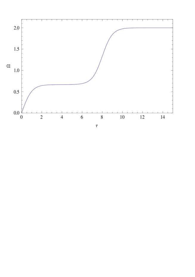
Figure 2: Vorticity $\Omega(\tau)$ plotted against $\tau$ with asymptotic value $\Omega_{c}$=2 and parameter $\tau_{0}$=8.

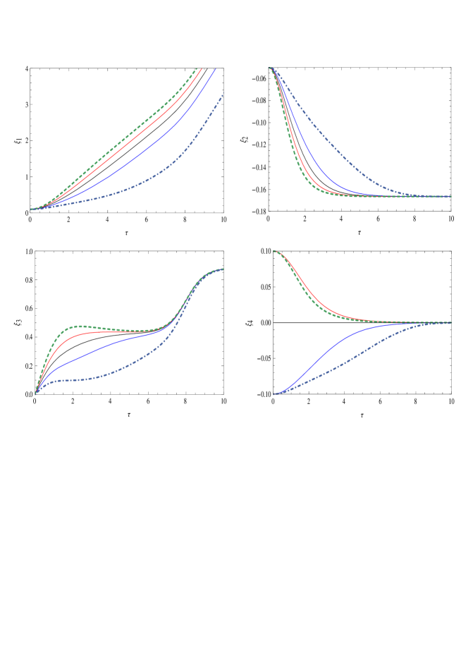
Figure 3: Variation of $\xi_{1}$, $\xi_{2}$, $\xi_{3}$, $\xi_{4}$ with $\tau$ for $r=1.5$, $V_{l}=0$, $\Omega_{c}=2$, $(\xi_{1})_{initial}=0.1$, $(\xi_{2})_{initial}=-0.05$ and $(\xi_{3})_{initial}=0$; ($V_{h}=0$, $(\xi_{4})_{initial}=0$( Black line), ($V_{h}=1$, $(\xi_{4})_{initial}=0.1$( Red line),($V_{h}=1$, $(\xi_{4})_{initial}=-0.1$( Blue line),($V_{h}=1.5$, $(\xi_{4})_{initial}=0.1$( Dash line),($V_{h}=1.5$, $(\xi_{4})_{initial}=-0.1$( Dot-dash line).

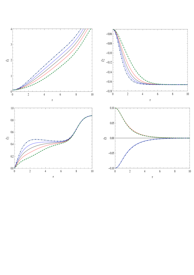
Figure 4: Variation of $\xi_{1}$, $\xi_{2}$, $\xi_{3}$, $\xi_{5}$ with $\tau$ for $r=1.5$, $V_{h}=0$, $\Omega_{c}=2$, $(\xi_{1})_{initial}=0.1$, $(\xi_{2})_{initial}=-0.05$ and $(\xi_{3})_{initial}=0$; ($V_{h}=l$, $(\xi_{5})_{initial}=0$( Black line), ($V_{l}=1$, $(\xi_{5})_{initial}=0.1$( Red line),($V_{l}=1$, $(\xi_{5})_{initial}=-0.1$( Blue line),($V_{l}=1.5$, $(\xi_{5})_{initial}=0.1$( Dash line),($V_{l}=1.5$, $(\xi_{5})_{initial}=-0.1$( Dot-dash line).

References

• [1] M.R.Gupta, L.Mandal, S.Roy, M.Khan, ”Effect of magnetic field on temporal development of Rayleigh Taylor instability induced interfacial nonlinear structure,” Phys. Plasmas 17, 012306 (2010).
• [2] S Chandrasekhar, ”Hydrodynamic and Hydromagnetic Stability,” (Dover,Newyork,1961).
• [3] D. Layzer,”On the instability of superposed fluids in a gravitational field,” Astrophys. J.122, 1 (1955).
• [4] V.N.Goncharov, ”Analytical Model of Nonlinear, Single-Mode, Classical Rayleigh-Taylor Instability at Arbitrary Atwood Numbers,” Phys. Rev. Lett.88, 134502 (2002).
• [5] P. Ramaprabhu, G. Dimonte, Yuan-Nan Young, A.C. Calder, B. Fryxell,”Limits of the potential flow approach to the single-mode Rayleigh-Taylor problem,” Phys. Rev. E 74, 066308 (2006).
• [6] R.Betti, J.Sanz, ”Bubble Acceleration in the Ablative Rayleigh-Taylor Instability,” Phys. Rev. Lett.97, 205002 (2006).
• [7] R. Banerjee, L.Mandal, S.Roy, M.Khan, M.R.Gupta,”Combined effect of viscosity and vorticity on single mode Rayleigh Taylor instability bubble growth,” Phys. Plasmas 18, 022109 (2011).
• [8] R. Banerjee, L.Mandal, M.Khan, M.R.Gupta, ”Effect of viscosity and shear flow on the nonlinear two fluid interfacial structures,” Phys. Plasmas19, 122105 (2012).
Refer to caption