UnitBox: An Advanced Object Detection Network

Abstract

In present object detection systems, the deep convolutional neural networks (CNNs) are utilized to predict bounding boxes of object candidates, and have gained performance advantages over the traditional region proposal methods. However, existing deep CNN methods assume the object bounds to be four independent variables, which could be regressed by the $\ell_{2}$ loss separately. Such an oversimplified assumption is contrary to the well-received observation, that those variables are correlated, resulting to less accurate localization. To address the issue, we firstly introduce a novel Intersection over Union ($IoU$) loss function for bounding box prediction, which regresses the four bounds of a predicted box as a whole unit. By taking the advantages of $IoU$ loss and deep fully convolutional networks, the UnitBox is introduced, which performs accurate and efficient localization, shows robust to objects of varied shapes and scales, and converges fast. We apply UnitBox on face detection task and achieve the best performance among all published methods on the FDDB benchmark.

1 Introduction

Visual object detection could be viewed as the combination of two tasks: object localization (where the object is) and visual recognition (what the object looks like). While the deep convolutional neural networks (CNNs) has witnessed major breakthroughs in visual object recognition [3] [11] [13], the CNN-based object detectors have also achieved the state-of-the-arts results on a wide range of applications, such as face detection [8] [5], pedestrian detection [9] [4] and etc [2] [1] [10].

Currently, most of the CNN-based object detection methods [2] [4] [8] could be summarized as a three-step pipeline: firstly, region proposals are extracted as object candidates from a given image. The popular region proposal methods include Selective Search [12], EdgeBoxes [15], or the early stages of cascade detectors [8]; secondly, the extracted proposals are fed into a deep CNN for recognition and categorization; finally, the bounding box regression technique is employed to refine the coarse proposals into more accurate object bounds. In this pipeline, the region proposal algorithm constitutes a major bottleneck in terms of localization effectiveness, as well as efficiency. On one hand, with only low-level features, the traditional region proposal algorithms are sensitive to the local appearance changes, e.g., partial occlusion, where those algorithms are very likely to fail. On the other hand, a majority of those methods are typically based on image over-segmentation [12] or dense sliding windows [15], which are computationally expensive and have hamper their deployments in the real-time detection systems.

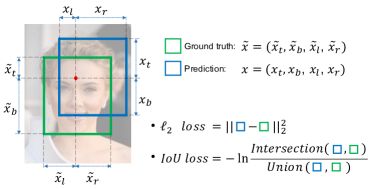
Figure 1: Illustration of $IoU$ loss and $\ell_{2}$ loss for pixel-wise bounding box prediction.

To overcome these disadvantages, more recently the deep CNNs are also applied to generate object proposals. In the well-known Faster R-CNN scheme [10], a region proposal network (RPN) is trained to predict the bounding boxes of object candidates from the anchor boxes. However, since the scales and aspect ratios of anchor boxes are pre-designed and fixed, the RPN shows difficult to handle the object candidates with large shape variations, especially for small objects.

Another successful detection framework, DenseBox [5], utilizes every pixel of the feature map to regress a 4-D distance vector (the distances between the current pixel and the four bounds of object candidate containing it). However, DenseBox optimizes the four-side distances as four independent variables, under the simplistic $\ell_{2}$ loss, as shown in Figure 1. It goes against the intuition that those variables are correlated and should be regressed jointly.

Besides, to balance the bounding boxes with varied scales, DenseBox requires the training image patches to be resized to a fixed scale. As a consequence, DenseBox has to perform detection on image pyramids, which unavoidably affects the efficiency of the framework.

The paper proposes a highly effective and efficient CNN-based object detection network, called UnitBox. It adopts a fully convolutional network architecture, to predict the object bounds as well as the pixel-wise classification scores on the feature maps directly. Particularly, UnitBox takes advantage of a novel Intersection over Union ($IoU$) loss function for bounding box prediction. The $IoU$ loss directly enforces the maximal overlap between the predicted bounding box and the ground truth, and jointly regress all the bound variables as a whole unit (see Figure 1). The UnitBox demonstrates not only more accurate box prediction, but also faster training convergence. It is also notable that thanks to the $IoU$ loss, UnitBox is enabled with variable-scale training. It implies the capability to localize objects in arbitrary shapes and scales, and to perform more efficient testing by just one pass on singe scale. We apply UnitBox on face detection task, and achieve the best performance on FDDB [6] among all published methods.

2 IoU Loss Layer

Before introducing UnitBox, we firstly present the proposed $IoU$ loss layer and compare it with the widely-used $\ell_{2}$ loss in this section. Some important denotations are claimed here: for each pixel $(i,j)$ in an image, the bounding box of ground truth could be defined as a 4-dimensional vector:

$$\boldsymbol{\widetilde{x}_{i,j}}=(\widetilde{x}_{t_{i,j}},\widetilde{x}_{b_{i,j}},\widetilde{x}_{l_{i,j}},\widetilde{x}_{r_{i,j}}),$$ (1)

where $\widetilde{x}_{t}$, $\widetilde{x}_{b}$, $\widetilde{x}_{l}$, $\widetilde{x}_{r}$ represent the distances between current pixel location $(i,j)$ and the top, bottom, left and right bounds of ground truth, respectively. For simplicity, we omit footnote $i,j$ in the rest of this paper. Accordingly, a predicted bounding box is defined as $\boldsymbol{x}=(x_{t},x_{b},x_{l},x_{r})$, as shown in Figure 1.

2.1 L2 Loss Layer

$\ell_{2}$ loss is widely used in optimization. In [5] [7], $\ell_{2}$ loss is also employed to regress the object bounding box via CNNs, which could be defined as:

$$\mathcal{L}(x,\widetilde{x})=\sum_{i\in\{t,b,l,r\}}{(x_{i}-\widetilde{x}_{i})^{2}},$$ (2)

where $\mathcal{L}$ is the localization error.

However, there are two major drawbacks of $\ell_{2}$ loss for bounding box prediction. The first is that in the $\ell_{2}$ loss, the coordinates of a bounding box (in the form of $x_{t}$, $x_{b}$, $x_{l}$, $x_{r}$) are optimized as four independent variables. This assumption violates the fact that the bounds of an object are highly correlated. It results in a number of failure cases in which one or two bounds of a predicted box are very close to the ground truth but the entire bounding box is unacceptable; furthermore, from Eqn. 2 we can see that, given two pixels, one falls in a larger bounding box while the other falls in a smaller one, the former will have a larger effect on the penalty than the latter, since the $\ell_{2}$ loss is unnormalized. This unbalance results in that the CNNs focus more on larger objects while ignore smaller ones. To handle this, in previous work [5] the CNNs are fed with the fixed-scale image patches in training phase, while applied on image pyramids in testing phase. In this way, the $\ell_{2}$ loss is normalized but the detection efficiency is also affected negatively.

2.2 IoU Loss Layer: Forward

In the following, we present a new loss function, named the $IoU$ loss, which perfectly addresses above drawbacks. Given a predicted bounding box $\boldsymbol{x}$ (after ReLU layer, we have $x_{t},x_{b},x_{l},x_{r}\geq 0$) and the corresponding ground truth $\boldsymbol{\widetilde{x}}$, we calculate the $IoU$ loss as follows:

Input: $\boldsymbol{\widetilde{x}}$ as bounding box ground truth

Input: $\boldsymbol{x}$ as bounding box prediction

Output: $\mathcal{L}$ as localization error

for each pixel $(i,j)$ do

      if $\boldsymbol{\widetilde{x}}\neq\boldsymbol{0}$ then

           $X=(x_{t}+x_{b})*(x_{l}+x_{r})$

           $\widetilde{X}=(\widetilde{x}_{t}+\widetilde{x}_{b})*(\widetilde{x}_{l}+\widetilde{x}_{r})$

           $I_{h}=min(x_{t},\widetilde{x}_{t})+min(x_{b},\widetilde{x}_{b})$

           $I_{w}=min(x_{l},\widetilde{x}_{l})+min(x_{r},\widetilde{x}_{r})$

           $I=I_{h}*I_{w}$

           $U=X+\widetilde{X}-I$

           $IoU=\dfrac{I}{U}$

           $\mathcal{L}=-ln(IoU)$

          

           else

                $\mathcal{L}=0$

                end if

               

                end for

Algorithm 1 $IoU$ loss Forward

In Algorithm 1, $\boldsymbol{\widetilde{x}}\neq\boldsymbol{0}$ represents that the pixel $(i,j)$ falls inside a valid object bounding box; $X$ is area of the predicted box; $\widetilde{X}$ is area of the ground truth box; $I_{h}$, $I_{w}$ are the height and width of the intersection area $I$, respectively, and $U$ is the union area.

Note that with $0\leq IoU\leq 1$, $\mathcal{L}=-ln(IoU)$ is essentially a cross-entropy loss with input of $IoU$: we can view $IoU$ as a kind of random variable sampled from Bernoulli distribution, with $p(IoU=1)=1$, and the cross-entropy loss of the variable $IoU$ is $\mathcal{L}=-pln(IoU)-(1-p)ln(1-IoU)=-ln(IoU)$. Compared to the $\ell_{2}$ loss, we can see that instead of optimizing four coordinates independently, the $IoU$ loss considers the bounding box as a unit. Thus the $IoU$ loss could provide more accurate bounding box prediction than the $\ell_{2}$ loss. Moreover, the definition naturally norms the $IoU$ to $[0,1]$ regardless of the scales of bounding boxes. The advantage enables UnitBox to be trained with multi-scale objects and tested only on single-scale image.

2.3 IoU Loss Layer: Backward

To deduce the backward algorithm of $IoU$ loss, firstly we need to compute the partial derivative of $X$ w.r.t. $x$, marked as $\nabla_{x}X$ (for simplicity, we notate $x$ for any of $x_{t}$, $x_{b}$, $x_{l}$, $x_{r}$ if missing):

$$\frac{\partial X}{\partial x_{t}(\textbf{or}\ \partial x_{b})}=x_{l}+x_{r},$$ (3)

$$\frac{\partial X}{\partial x_{l}(\textbf{or}\ \partial x_{r})}=x_{t}+x_{b}.$$ (4)

To compute the partial derivative of $I$ w.r.t $x$, marked as $\nabla_{x}I$:

$$\frac{\partial I}{\partial x_{t}(\textbf{or}\ \partial x_{b})}=\begin{cases}I_{w},&\text{if}\ x_{t}<\widetilde{x}_{t}(\textbf{or}\ x_{b}<\widetilde{x}_{b})\\ 0,&\text{otherwise},\end{cases}$$ (5)

$$\frac{\partial I}{\partial x_{l}(\textbf{or}\ \partial x_{r})}=\begin{cases}I_{h},&\text{if}\ x_{l}<\widetilde{x}_{l}(\textbf{or}\ x_{r}<\widetilde{x}_{r})\\ 0,&\text{otherwise}.\end{cases}$$ (6)

Finally we can compute the gradient of localization loss $\mathcal{L}$ w.r.t. $x$:

$$\begin{split}\frac{\partial{\mathcal{L}}}{\partial x}&=\frac{I(\nabla_{x}X-\nabla_{x}I)-U\nabla_{x}I}{U^{2}IoU}\\ &=\frac{1}{U}\nabla_{x}X-\frac{U+I}{UI}\nabla_{x}I.\end{split}$$ (7)

From Eqn. 7, we can have a better understanding of the $IoU$ loss layer: the $\nabla_{x}X$ is the penalty for the predict bounding box, which is in a positive proportion to the gradient of loss; and the $\nabla_{x}I$ is the penalty for the intersection area, which is in a negative proportion to the gradient of loss. So overall to minimize the $IoU$ loss, the Eqn. 7 favors the intersection area as large as possible while the predicted box as small as possible. The limiting case is the intersection area equals to the predicted box, meaning a perfect match.

3 UnitBox Network

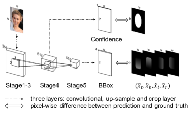
Figure 2: The Architecture of UnitBox Network.

Based on the $IoU$ loss layer, we propose a pixel-wise object detection network, named UnitBox. As illustrated in Figure 2, the architecture of UnitBox is derived from VGG-16 model [11], in which we remove the fully connected layers and add two branches of fully convolutional layers to predict the pixel-wise bounding boxes and classification scores, respectively. In training, UnitBox is fed with three inputs in the same size: the original image, the confidence heatmap inferring a pixel falls in a target object (positive) or not (negative), and the bounding box heatmaps inferring the ground truth boxes at all positive pixels.

To predict the confidence, three layers are added layer-by-layer at the end of VGG stage-4: a convolutional layer with stride $1$, kernel size $512\times 3\times 3\times 1$; an up-sample layer which directly performs linear interpolation to resize the feature map to original image size; a crop layer to align the feature map with the input image. After that, we obtain a 1-channel feature map with the same size of input image, on which we use the sigmoid cross-entropy loss to regress the generated confidence heatmap; in the other branch, to predict the bounding box heatmaps we use the similar three stacked layers at the end of VGG stage-5 with convolutional kernel size 512 x 3 x 3 x 4. Additionally, we insert a ReLU layer to make bounding box prediction non-negative. The predicted bounds are jointly optimized with $IoU$ loss proposed in Section 2. The final loss is calculated as the weighted average over the losses of the two branches.

Some explanations about the architecture design of UnitBox are listed as follows: 1) in UnitBox, we concatenate the confidence branch at the end of VGG stage-4 while the bounding box branch is inserted at the end of stage-5. The reason is that to regress the bounding box as a unit, the bounding box branch needs a larger receptive field than the confidence branch. And intuitively, the bounding boxes of objects could be predicted from the confidence heatmap. In this way, the bounding box branch could be regarded as a bottom-up strategy, abstracting the bounding boxes from the confidence heatmap; 2) to keep UnitBox efficient, we add as few extra layers as possible. Compared to DenseBox [5] in which three convolutional layers are inserted for bounding box prediction, the UnitBox only uses one convolutional layer. As a result, the UnitBox could process more than 10 images per second, while DenseBox needs several seconds to process one image; 3) though in Figure 2 the bounding box branch and the confidence branch share some earlier layers, they could be trained separately with unshared weights to further improve the effectiveness.

With the heatmaps of confidence and bounding box, we can now accurately localize the objects. Taking the face detection for example, to generate bounding boxes of faces, firstly we fit the faces by ellipses on the thresholded confidence heatmaps. Since the face ellipses are too coarse to localize objects, we further select the center pixels of these coarse face ellipses and extract the corresponding bounding boxes from these selected pixels. Despite its simplicity, the localization strategy shows the ability to provide bounding boxes of faces with high accuracy, as shown in Figure 3.

4 Experiments

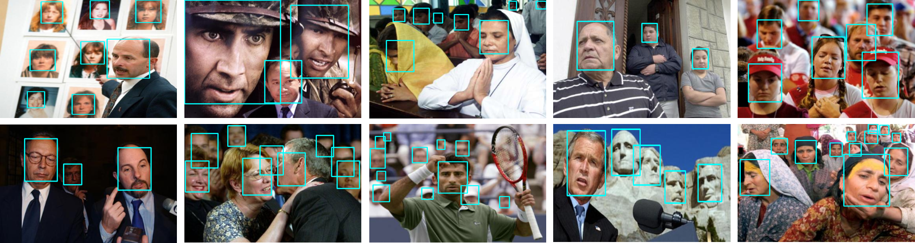
Figure 3: Examples of detection results of UnitBox on FDDB.

In this section, we apply the proposed $IoU$ loss as well as the UnitBox on face detection task, and report our experimental results on the FDDB benchmark [6]. The weights of UnitBox are initialized from a VGG-16 model pre-trained on ImageNet, and then fine-tuned on the public face dataset WiderFace [14]. We use mini-batch SGD in fine-tuning and set the batch size to 10. Following the settings in [5], the momentum and the weight decay factor are set to 0.9 and 0.0002, respectively. The learning rate is set to $10^{-8}$ which is the maximum trainable value. No data augmentation is used during fine-tuning.

4.1 Effectiveness of IoU Loss

First of all we study the effectiveness of the proposed $IoU$ loss. To train a UnitBox with $\ell_{2}$ loss, we simply replace the $IoU$ loss layer with the $\ell_{2}$ loss layer in Figure 2, and reduce the learning rate to $10^{-13}$ (since $\ell_{2}$ loss is generally much larger, $10^{-13}$ is the maximum trainable value), keeping the other parameters and network architecture unchanged. Figure 4(a) compares the convergences of the two losses, in which the X-axis represents the number of iterations and the Y-axis represents the detection miss rate. As we can see, the model with $IoU$ loss converges more quickly and steadily than the one with $\ell_{2}$ loss. Besides, the UnitBox has a much lower miss rate than the UnitBox-$\ell_{2}$ throughout the fine-tuning process.

In Figure 4(b), we pick the best models of UnitBox ($\sim$ 16k iterations) and UnitBox-$\ell_{2}$ ($\sim$ 29k iterations), and compare their ROC curves. Though with fewer iterations, the UnitBox with $IoU$ loss still significantly outperforms the one with $\ell_{2}$ loss.

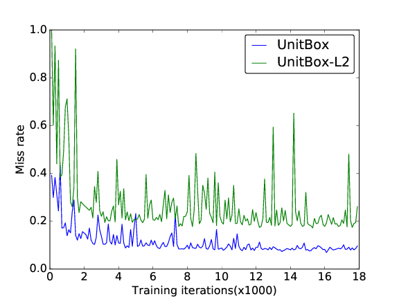
(a) Convergence

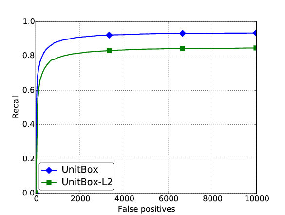
(b) ROC Curves

Figure 4: Comparison: $IoU$ vs. $\ell_{2}$.

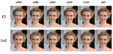
Figure 5: Compared to $\ell_{2}$ loss, the $IoU$ loss is much more robust to scale variations for bounding box prediction.

Moreover, we study the robustness of $IoU$ loss and $\ell_{2}$ loss to the scale variation. As shown in Figure 5, we resize the testing images from 60 to 960 pixels, and apply UnitBox and UnitBox-$\ell_{2}$ on the image pyramids. Given a pixel at the same position (denoted as the red dot), the bounding boxes predicted at this pixel are drawn. From the result we can see that 1) as discussed in Section  2.1, the $\ell_{2}$ loss could hardly handle the objects in varied scales while the $IoU$ loss works well; 2) without joint optimization, the $\ell_{2}$ loss may regress one or two bounds accurately, e.g., the up bound in this case, but could not provide satisfied entire bounding box prediction; 3) in the x960 testing image, the face size is even larger than the receptive fields of the neurons in UnitBox (around 200 pixels). Surprisingly, the UnitBox can still give a reasonable bounding box in the extreme cases while the UnitBox-$\ell_{2}$ totally fails.

4.2 Performance of UnitBox

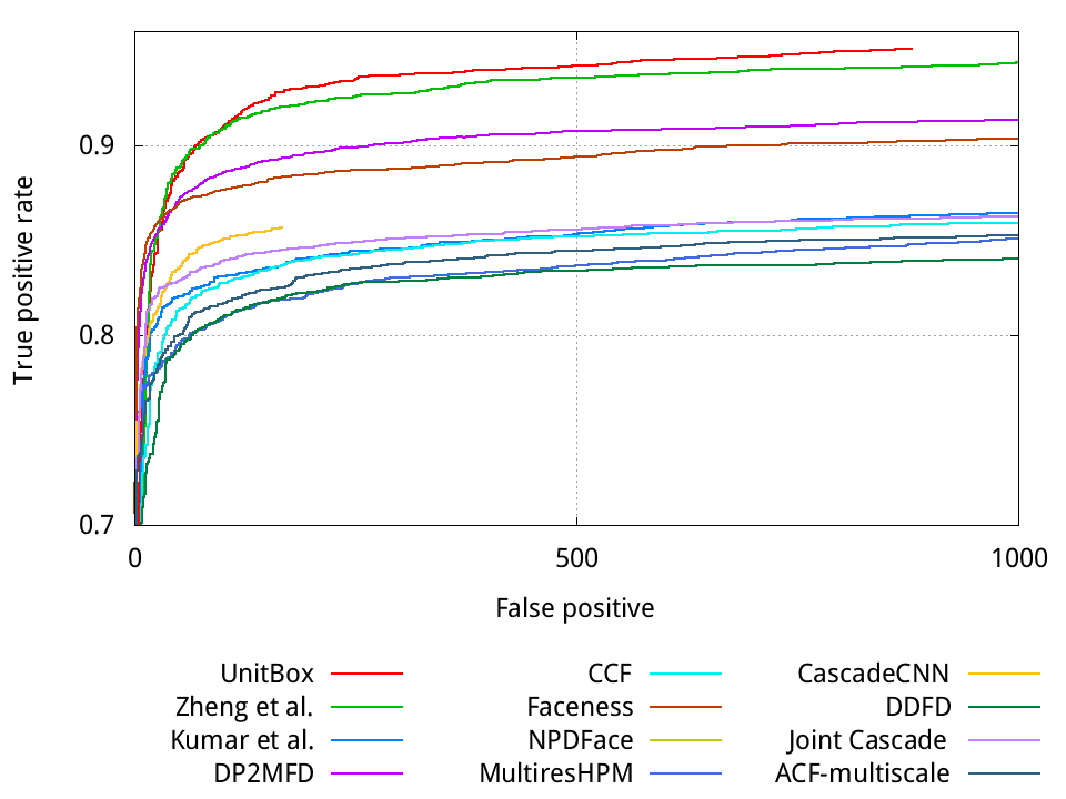
Figure 6: The Performance of UnitBox comparing with state-of-the-arts Methods on FDDB.

To demonstrate the effectiveness of the proposed method, we compare the UnitBox with the state-of-the-arts methods on FDDB. As illustrated in Section 3, here we train an unshared UnitBox detector to further improve the detection performance. The ROC curves are shown in Figure 6. As a result, the proposed UnitBox has achieved the best detection result on FDDB among all published methods.

Except that, the efficiency of UnitBox is also remarkable. Compared to the DenseBox [5] which needs seconds to process one image, the UnitBox could run at about 12 fps on images in VGA size. The advantage in efficiency makes UnitBox potential to be deployed in real-time detection systems.

5 Conclusions

The paper presents a novel loss, i.e., the $IoU$ loss, for bounding box prediction. Compared to the $\ell_{2}$ loss used in previous work, the $IoU$ loss layer regresses the bounding box of an object candidate as a whole unit, rather than four independent variables, leading to not only faster convergence but also more accurate object localization. Based on the $IoU$ loss, we further propose an advanced object detection network, i.e., the UnitBox, which is applied on the face detection task and achieves the state-of-the-art performance. We believe that the $IoU$ loss layer as well as the UnitBox will be of great value to other object localization and detection tasks.

References

- [1] V. Belagiannis, X. Wang, H. Beny Ben Shitrit, K. Hashimoto, R. Stauder, Y. Aoki, M. Kranzfelder, A. Schneider, P. Fua, S. Ilic, H. Feussner, and N. Navab. Parsing human skeletons in an operating room. Machine Vision and Applications, 2016.
- [2] R. Girshick, J. Donahue, T. Darrell, and J. Malik. Rich feature hierarchies for accurate object detection and semantic segmentation. In Computer Vision and Pattern Recognition, 2014.
- [3] K. He, X. Zhang, S. Ren, and J. Sun. Deep Residual Learning for Image Recognition. ArXiv e-prints, Dec. 2015.
- [4] J. Hosang, M. Omran, R. Benenson, and B. Schiele. Taking a deeper look at pedestrians. In Proceedings of the IEEE Conference on Computer Vision and Pattern Recognition, pages 4073–4082, 2015.
- [5] L. Huang, Y. Yang, Y. Deng, and Y. Yu. DenseBox: Unifying Landmark Localization with End to End Object Detection. ArXiv e-prints, Sept. 2015.
- [6] V. Jain and E. Learned-Miller. Fddb: A benchmark for face detection in unconstrained settings. Technical Report UM-CS-2010-009, University of Massachusetts, Amherst, 2010.
- [7] Z. Jie, X. Liang, J. Feng, W. F. Lu, E. H. F. Tay, and S. Yan. Scale-aware Pixel-wise Object Proposal Networks. ArXiv e-prints, Jan. 2016.
- [8] H. Li, Z. Lin, X. Shen, J. Brandt, and G. Hua. A convolutional neural network cascade for face detection. In Proceedings of the IEEE Conference on Computer Vision and Pattern Recognition, pages 5325–5334, 2015.
- [9] J. Li, X. Liang, S. Shen, T. Xu, and S. Yan. Scale-aware Fast R-CNN for Pedestrian Detection. ArXiv e-prints, Oct. 2015.
- [10] S. Ren, K. He, R. Girshick, and J. Sun. Faster R-CNN: Towards real-time object detection with region proposal networks. In Advances in Neural Information Processing Systems (NIPS), 2015.
- [11] K. Simonyan and A. Zisserman. Very Deep Convolutional Networks for Large-Scale Image Recognition. ArXiv e-prints, Sept. 2014.
- [12] J. R. R. Uijlings, K. E. A. van de Sande, T. Gevers, and A. W. M. Smeulders. Selective search for object recognition. International Journal of Computer Vision, 104(2):154–171, 2013.
- [13] Z. Wang, S. Chang, Y. Yang, D. Liu, and T. S. Huang. Studying very low resolution recognition using deep networks. CoRR, abs/1601.04153, 2016.
- [14] S. Yang, P. Luo, C. C. Loy, and X. Tang. Wider face: A face detection benchmark. In IEEE Conference on Computer Vision and Pattern Recognition (CVPR), 2016.
- [15] C. L. Zitnick and P. Dollár. Edge boxes: Locating object proposals from edges. In ECCV. European Conference on Computer Vision, September 2014.