Temperature of a single chaotic eigenstate

Abstract

The onset of thermalization in a closed system of randomly interacting bosons, at the level of a single eigenstate, is discussed. We focus on the emergence of Bose-Einstein distribution of single-particle occupation numbers, and we give a local criterion for thermalization dependent on the eigenstate energy. We show how to define the temperature of an eigenstate, provided that it has a chaotic structure in the basis defined by the single-particle states. The analytical expression for the eigenstate temperature as a function of both inter-particle interaction and energy is complemented by numerical data.

I Introduction

The subject of thermalization occurring in isolated quantum systems of interacting particles has been developed the last decades due to various applications in nuclear and atomic physics zele ; flam , as well as in view of basic problems of statistical mechanics rep ; basic ; basic1 . Recently the interest to this subject has increased due to experiments with cold atoms and molecules in optical lattices exp and trapped ions exp1 . Correspondingly, many theoretical and numerical studies have been performed in order to understand the mechanism of thermalization in the absence of a heat bath (see  rep and Refs therein). Nevertheless, despite some studies about the onset of thermalization as a function of various physical parameters such as the number of particlesmanan , the strength of inter-particle interactionour2012 , the choice of initially excited states leajon , the role of these items still remains open.

The mechanism driving thermalization in isolated systems of interacting particles is associated with quantum chaos our2016 . Differently from the well developed one-body chaos theory, many problems related to many-body chaos, such as the thermalization of Fermi and Bose particles, are currently under intensive studies. Unlike classical chaos which is intrinsically related to the instability of motion with respect to a change of initial conditions, quantum chaos manifests itself in specific fluctuations of the energy spectra and in the chaotic structure of eigenstates. As shown in our2012 , the properties of the energy spectra are less important to the statistical relaxation toward a steady-state distribution than the structure of the eigenstates in the physically chosen many-particle basis. Therefore, the main interest in the study of many-body chaos was shifted, since long, to the properties of many-body eigenstates.

Chaotic eigenstates play a key role in the statistical description of isolated quantum systems. As stressed long ago Landau , conventional statistical mechanics can be established on the level of individual quantum states and not only by averaging over many states. This has been confirmed numerically decades ago, see for instance our2016 and discussion in jen . However, this fact has no practical consequences unless the conditions for such a situation are developed. One of the open problems in this field is to establish these conditions for systems with a finite number of particles.

To date, many problems have been addressed concerning the problem of thermalization in isolated systems. Here we raise a new one, which is directly related to this issue. It is already agreed that one can speak of thermalization on the level of an individual state, and various characteristics of thermalization have been under extensive studies, such as the relaxation of a system to steady state distributions after various quenches, decay of correlations in time for observables and their fluctuations after relaxation, etc. exp ; exp1 ; BBIS04 ; manan ; leajon ; our2012 .

Now, in view of the basic concepts of statistical mechanics and recent experiments with cold atoms and moleculesexp it is natural to ask the question about the onset of the Bose-Einstein distribution (BED) emerging on the level of a single many-body eigenstate, due to the interaction between bosons and not to an external field or a thermostat. Below we specifically initiate the study of the onset of BED in a finite system of interacting bosons, that is expected to occur when the inter-particle interaction is strong enough. We suggest a semi-analytical approach able to reveal the conditions under which an isolated many-body eigenstate can be considered thermal and introduce its temperature in relation to the model parameters.

II The model and basic concepts

At variance with eigenvalues, many-particle eigenstates are defined by means of a suitable single-particle basis. The latter, from its side has a direct relevance to the physical reality, specifically, to the choice of the mean field to which quantum observables such as occupation numbers are referred to. Correspondingly, we assume that the total Hamiltonian $H$ can be presented as the sum of the mean field $H_{0}$ describing non-interacting (quasi) particles, and a residual interaction $V$, modeled as a two-body random interaction. Such a setup, based on a random interaction, also serves as a good model for a deterministic interaction between bosonsBBIS04 where the complexity in many-body matrix elements emerges due to the complicated nature of the interaction itself.

In this paper we consider $N$ identical bosons occupying $M$ single-particle levels specified by random energies $\epsilon_{s}$ with mean spacing, $\langle\epsilon_{s}-\epsilon_{s-1}\rangle=1$. Let us notice that the randomness in the single particle spectrum is not strictly necessary for the results obtained: it has been introduced only in order to avoid the degeneracies in the unperturbed many-body spectrum.

The Hamiltonian reads

$$H=H_{0}+V=\sum_{s}\epsilon_{s}\,a^{\dagger}_{s}a_{s}+\sum_{s_{1}s_{2}s_{3}s_{4}}V_{s_{1}s_{2}s_{3}s_{4}}\,a^{\dagger}_{s_{1}}a^{\dagger}_{s_{2}}a_{s_{3}}a_{s_{4}}$$ (1)

where the two-body matrix elements $V_{s_{1}s_{2}s_{3}s_{4}}$ are random Gaussian entries with zero mean and variance $V^{2}$. The dimension of the Hilbert space generated by the many-particle basis states is ${N_{H}}=(N+M-1)!/N!(M-1)!$. Here we consider $N=6$ particles in $M=11$ levels (dilute limit, $N\leq M$) for which $N_{H}=8008$.

Two-body random interaction (TBRI) matrices (1) have a quite long history. They were introduced in TBRI and extensively studied for fermions fermi . On the other hand the case of Bose particles has been less investigated and only few results are known and typically for the dense limit, $N\gg M$ bosons ; kota-bose .

The eigenstates of $H$ can be generically represented in terms of the basis states $|k\rangle=a^{\dagger}_{k_{1}}...a^{\dagger}_{k_{N}}|0\rangle$ which are eigenstates of $H_{0}$,

$$\left|\alpha\,\right\rangle=\sum_{k}C_{k}^{\alpha}\left|k\,\right\rangle,$$ (2)

where it has been implicitly assumed that

$$H|\alpha\rangle=E^{\alpha}|\alpha\rangle,$$ (3)

and

$$H_{0}|k\rangle=E^{0}_{k}|k\rangle.$$ (4)

A characterization of the number of principal components $C_{k}^{\alpha}$ in an eigenstate $\left|\alpha\,\right\rangle$ can be obtained by the study of the participation ratio,

$$N_{pc}=1/\sum_{k}|C_{k}^{\alpha}|^{4}.$$ (5)

If the number $N_{pc}$ of the principal components $C_{k}^{\alpha}$ is sufficiently large (we will specify later how much large it should be) and $C_{k}^{\alpha}$ can be considered as random and non-correlated ones, this is the case of chaotic eigenstates. This notion is quite different from full delocalization in the unperturbed basis since for isolated systems the eigenstates typically fill only a part of the unperturbed basis our2016 .

To characterize the structure of the eigenstates, we use the $F-$function,

$$F^{\alpha}(E)=\sum_{k}|C_{k}^{\alpha}|^{2}\delta(E-E^{0}_{k}),$$ (6)

which is the energy representation of an eigenstate. From the components $C_{k}^{\alpha}$ one can also construct the strength function (SF) of a basis state $\left|k\,\right\rangle$,

$$F_{k}(E)=\sum_{\alpha}|C^{\alpha}_{k}|^{2}\delta(E-E^{\alpha})$$ (7)

widely used in nuclear physics SF and known in solid state physics as local density of states. The SF shows how the basis state $\left|k\,\right\rangle$ decomposes into the exact eigenstates $\left|\alpha\,\right\rangle$ due to the interaction $V$. It can be measured experimentally and it is of great importance since its Fourier transform gives the time evolution of an excitation initially concentrated in the basis state $\left|k\,\right\rangle$. Specifically, it defines the survival probability to find the system at time $t$ in the initial state $\left|k\,\right\rangle$.

On increasing the interaction strength, the SF in isolated systems undergoes a crossover from a delta-like function (perturbative regime) to a Breit-Wigner (BW), with a width well described by the Fermi golden rule. With a further increase of the interaction, the form of the SF tends to a Gaussianbasic ; our2012 ; ljnjp , a scenario that has also been observed experimentally horacio .

One of the basic concepts in our approach is the so-called energy shell which is the energy region defined by the projection of $V$ onto the basis of $H_{0}$ chirikov . This region is the largest one that can be occupied by an eigenstate. The partial filling of the energy shell by an eigenstate can be associated with the many-body localization in the energy representation, a subject that is nowadays under intensive investigation (see, for example, MBL and references therein). When this happens, of course, the eigenstates cannot be treated as thermal, in the sense that a good definition of temperature cannot be done. Contrary to this, if a chaotic eigenstate fills completely the energy shell, this corresponds to maximal quantum chaos, and a proper temperature can be defined.

In the past a parameter driving the global crossover from non-chaotic to chaotic eigenstates has been proposed based essentially on the ratio between the interaction strength and the mean energy range spanned by the basis states effectively coupled by the interaction $V$basic ; basic1 ; our2016 . This criterion is independent of the energy of the eigenstate. Since we are dealing here with single eigenstates we will generalize this idea in order to obtain a local criterion (i.e. depending on the eigenenergy) for such a crossover.

Each many–body eigenstate $\left|\alpha\,\right\rangle$ is not only characterized by an “effective number” of occupied basis states, $N_{pc}$ i.e. a number of principal components in the unperturbed basis, but also by an unperturbed energy width,

$$\delta_{0}=\left(\left\langle\alpha\,\right|H_{0}^{2}\left|\alpha\,\right\rangle-\left\langle\alpha\,\right|H_{0}\left|\alpha\,\right\rangle^{2}\right)^{1/2}.$$ (8)

These two parameters allow to define, for each single eigenstate, an effective mean energy spacing, $d_{loc}=\delta_{0}/N_{pc}$, that the perturbation strength $V$ must overcome in order to go beyond the perturbative regime. Accordingly, in order to have chaotic eigenstates we require $V>d_{loc}$, while for $V<d_{loc}$ we can speak of perturbative regime. In the following we will see that the region characterized by $V>d_{loc}$ is the “thermal ” one, where an effective temperature, dependent on the inter-particle interaction, can be defined via the Bose-Einstein distribution.

III The Bose-Einstein distribution for an interacting eigenstate

In order to define the temperature for each selected eigenstate $|\alpha\rangle$ let us consider its occupation number distribution (OND),

$$n_{s}^{\alpha}=\langle\alpha|\hat{n}_{s}|\alpha\rangle=\sum_{k}|C_{k}^{\alpha}|^{2}\langle k|\hat{n}_{s}|k\rangle.$$ (9)

As one can see, the OND (9) consists of two ingredients: the probabilities $|C_{k}^{\alpha}|^{2}$ and the occupation numbers $\langle k|\hat{n}_{s}|k\rangle$ related to the basis states of $H_{0}$. The latter are just integer numbers $0,1,2,...N$ depending on how many bosons occupy the single-particle level $s$ with respect to the many-body state $|k\rangle$. If the eigenstate $|\alpha\rangle$ of $H$ consists of many uncorrelated components one can substitute $|C_{k}^{\alpha}|^{2}$ by the corresponding SF obtained either by an average over a number of eigenstates with close energies, or inside an individual eigenstate, for example, with the use of the “moving window” average our2016 . Thus, from the knowledge of the SF it is possible to obtain the OND without the diagonalization of huge Hamiltonian matrices.

Having in mind to define the temperature of a single eigenstate by means of its corresponding OND, few relevant questions come out. First of all, since we are dealing with bosons, the common reference OND is the Bose-Einstein distribution (BED) that is derived for non-interacting particles in the thermodynamic limit. The situation here is clearly different since our system has a finite number of interacting particles. To address properly this question we start with the basic relations,

$$\sum_{s}n_{s}=N\qquad\sum_{s}\epsilon_{s}n_{s}=E,$$ (10)

where $N$ is the total number of bosons and $E$ is the energy of a system for which the inter-particle interaction is neglected. As is known, the solution of these equations for $N\rightarrow\infty$ leads to the BED,

$$n_{s}^{BE}=(e^{\beta(\epsilon_{s}-\mu)}-1)^{-1}.$$ (11)

The derivation can be obtained due to the combinatorics only, with the constants $\beta$ and $\mu$ as the Lagrange multipliers RR80 (see, also, discussion in Ref.TYW16 ). The meaning of $\beta$ and $\mu$ as the inverse temperature and chemical potential respectively, emerges when the system is connected with a heat bath. However, we will show that one can speak of BED even if the system is isolated; moreover, this distribution emerges on the level of a single eigenstate of the total Hamiltonian. Inserting (11) into (10), one can obtain both $\beta$ and $z=e^{\beta\mu}$ as a function of $N$ and $E$. If we further fix the number of particles $N$ we obtain two functions $z(E)$ and $\beta(E)$, as shown in Fig. 1. The values of $z$ and $\beta$ correspondent to the energy $E^{\alpha}$ are indicated in Fig. 1 by empty circles that are obtained by the intersection of the vertical line $E=E^{\alpha}$ with the curves $z(E)$ and $\beta(E)$. Let us note that the BED indicated by a dashed line in Fig. 2 d) has been obtained using exactly these values of $z$ and $\beta$.

Now the key question is: what energy in the r.h.s. of Eq. (10) should be used for interacting bosons in order to have, if any, the correspondence to the numerically obtained OND fausto ?

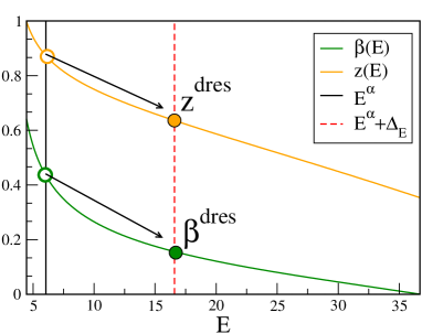
Figure 1: (Color online) Pictorial description of the increase of temperature for the eigenstate d) in Fig. 2.

First, we start with the global correspondence between the actual OND numerically obtained from individual eigenstates (9) and the BED expression (11). For this we consider the OND averaged over a number of close eigenstates in a narrow energy window. We considered the average over a small energy window with the only purpose to study fluctuations in the next section. In any case the OND’s for single eigenstates are shown in Fig.6 in Appendix.

We choose the eigenenergy $E^{\alpha}$ in two different regions: close to the center and to the edges of the spectrum, and, for each of them, two different values of the interaction strength $V$, see Fig. 2. In each panel of this figure the average values for the OND are shown with the error bars representing one standard deviation (fluctuations here are due to different eigentates in a close energy window, alternatively one can choose one single eigenstate and change the random inter-particle potential) and two curves, dashed and full. The dashed curves are those obtained by choosing as $E_{\alpha}$ the unperturbed energy while the full ones are obtained by “dressing” the energy, as shown here below.

As one can see in Fig. 2, while for weak interaction (top panels) dashed lines match perfectly numerical data, this does not happen for strong interaction (bottom panels). While such a failure in case of strong interaction is not unexpected, the good agreement in the case of weak interaction is far from trivial, since, it is worth noting that the Bose-Einstein distribution is obtained in the limit $N\to\infty$ while here we have only $N=6$ particles!

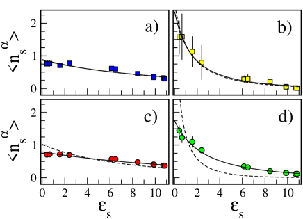
Figure 2: (Color online) Average occupation numbers $\langle n_{s}^{\alpha}\rangle$ for weak ($V=0.1$, top panels) and strong ($V=0.4$, bottom panels) perturbation and different energies: middle of the energy spectrum : a) $E^{\alpha}=28.51$, c) $E^{\alpha}=25.93$; edges : b) $E^{\alpha}=11.27$ and d) $E^{\alpha}=6.05$. Error bars indicate one standard deviation and are obtained by averaging over 20 close eigenstates. Dashed curves are obtained from the BED with $E=E^{\alpha}$ in Eq. (10). Full curves correspond to the BED with the energy $E^{dres}$ in Eq. (12).

To take into account the inter-particle interaction we use the approach suggested in Refs basic ; basic1 . Specifically, we substitute the energy $E=E^{\alpha}$ in (10) with the ”dressed” energy,

$$E^{dres}=\langle\alpha|H_{0}|\alpha\rangle\equiv E^{\alpha}+\Delta_{\alpha}.$$ (12)

Note that this energy is higher (in the region in which the density of states (DOS) increases with energy) than the eigenvalue $E^{\alpha}$ corresponding to the eigenstate $\left|\alpha\,\right\rangle$. This corresponds to a temperature $T^{dres}$ higher than that obtained with the substitution $E\to E^{\alpha}$. The dressed energy $E^{dres}=E^{\alpha}+\Delta_{\alpha}$ has been indicated as a vertical dashed line in Fig. 1. Since the energy shift $\Delta_{\alpha}$ is always positive in the energy region where the density of states increases with the energy, this produces a lowering of both $z$ and $\beta$ indicated in Fig. 1 as full circles ($z^{dres}$ and $\beta^{dres}$).

Plugging the BED , Eq. (11), in Eq. (10) with the substitution $E^{dres}\to E$ returns the values of $\mu$ and $\beta$ from which we can write down the corresponding BED indicated by full curves in Fig. 2. Even if, in the case of weak interaction (top column), the BED is hardly distinguishable from the “unperturbed one”, for strong interaction (bottom panels) they are very different, nevertheless, they match the numerical data extremely well, without any fit!

The energy shifts $\Delta_{\alpha}$ can be easily calculated numerically for each eigenstate. In Fig. 3 we plot such values, averaged over close eigenstates for the two different perturbation strengths $V$ considered in Fig. 2.

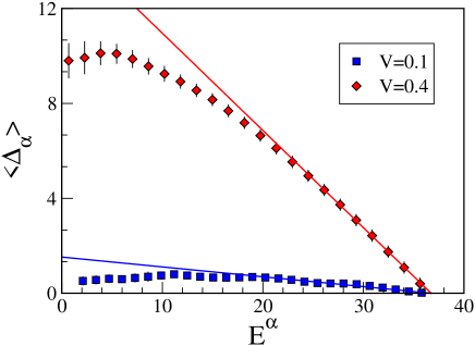
Figure 3: (Color online) Average energy shift $\langle\Delta_{\alpha}\rangle$ as a function of the energy $E^{\alpha}$ for two different values of the interaction $V$. Symbols stand for numerical results while full lines represent the Gaussian approximation. (error bars indicate one standard deviation). Average has been done over $20$ close eigenstates. Due to the symmetry only half of the energy spectrum (where the density of states is an increasing function of the energy) is shown.

It is also possible to derive an analytical expression for the energy shift $\Delta_{\alpha}$ in Eq. (12) under not too strong assumptions. For weak TBRI and a large number of particles, the form of the density of states (DOS) is a Gaussian gauss . Moreover, due to the trace conservation of $H$, the position of the center $E_{c}$ of the perturbed spectrum is the same of the unperturbed one. In this situation the variance $\sigma_{E}$ of the “perturbed” DOS $\rho$ is related to the variance $\sigma_{0}$ of the “unperturbed” DOS $\rho_{0}$ according to the simple relation (see Appendix for details)

$$\sigma_{E}^{2}=\sigma_{0}^{2}+\mkern 1.5mu\overline{\mkern-1.5mu(\Delta E)\mkern-1.5mu}\mkern 1.5mu^{2}$$ (13)

where

$$\mkern 1.5mu\overline{\mkern-1.5mu(\Delta E)^{2}\mkern-1.5mu}\mkern 1.5mu=(1/N_{H})\sum_{n}\sum_{k\neq n}H^{2}_{nk}$$ (14)

is the average width of the SF and it can be obtained without any diagonalization. Inserting in Eq. (12), the spectral decomposition of $H_{0}$,

$$H_{0}=\sum_{k}E^{0}_{k}|k\rangle\langle k|$$ (15)

one has,

$$\Delta_{\alpha}=\sum_{k}E^{0}_{k}|C_{k}^{\alpha}|^{2}-E^{\alpha}\simeq\int dE(E-E^{\alpha})\rho_{0}(E)\langle|C_{k}^{\alpha}|^{2}\rangle.$$ (16)

Assuming a Gaussian form also for $\langle|C_{k}^{\alpha}|^{2}\rangle$ peaked around $E^{\alpha}$,

$$\langle|C_{k}^{\alpha}|^{2}\rangle\simeq\exp[-(E-E^{\alpha})^{2}/2\mkern 1.5mu\overline{\mkern-1.5mu(\Delta E)^{2}\mkern-1.5mu}\mkern 1.5mu]$$ (17)

and for $\rho_{0}(E)$,

$$\rho_{0}(E)\simeq\exp[-(E-E_{c})^{2}/2\sigma_{0}^{2}]$$ (18)

and inserting in Eq. (16) with the correct normalizations, one gets the analytical estimate for the energy shift:

$$\Delta_{\alpha}=\displaystyle\frac{\mkern 1.5mu\overline{\mkern-1.5mu(\Delta E)\mkern-1.5mu}\mkern 1.5mu^{2}}{\mkern 1.5mu\overline{\mkern-1.5mu(\Delta E)\mkern-1.5mu}\mkern 1.5mu^{2}+\sigma_{0}^{2}}\left(E_{c}-E^{\alpha}\right)$$ (19)

These analytical values have been shown in Fig. 3 as solid lines. As one can see they work very well in the center of the energy spectrum (where the hypothesis of Gaussian LDOS and DOS can be applied without appreciable errors) while significant deviations appear at the low edge of the spectrum, where, due to the finite number of particles and levels it is well known that both DOS and LDOS cannot be described by Gaussians.

The increase of temperature, $\Delta T$, emerging due to the inter-particle interaction, can be obtained from the definition of thermodynamic temperature, by means of the unperturbed density of states $\rho_{0}$,

$$\beta=\frac{1}{T}=\frac{d\ln\rho_{0}}{dE}$$

so that

$$T^{dres}\equiv T+\Delta T=\left(\frac{d\ln\rho}{dE}\right)^{-1}=\frac{\sigma_{E}^{2}}{E_{c}-E}$$ (20)

and finally, from Eq. (13)

$$\frac{\Delta T}{T}=\frac{\mkern 1.5mu\overline{\mkern-1.5mu(\Delta E)^{2}\mkern-1.5mu}\mkern 1.5mu}{\sigma_{0}^{2}}.$$ (21)

As one can see, the relative shift of temperature turns out to be independent of the eigenenergy $E^{\alpha}$ and dependent only on the ratio between the variance $\sigma_{0}^{2}$ of the unperturbed DOS and the average variance $\mkern 1.5mu\overline{\mkern-1.5mu(\Delta E)^{2}\mkern-1.5mu}\mkern 1.5mu$ of the SF. Again, both can be found without the diagonalization of $H$. The analytical values of the temperature shift for the eigenstates in Fig. 2 agree fairly well with those obtained with the use of the energy shifts from Eq. (12) when the eigenenergy is far from the edges of the spectrum (top panels in Fig. 2). All numerical values of the shifts are reported for the reader convenience in Table I.

Table 1: Parameters for Fig. 2 of the main text. $E^{\alpha}$ is the eigenenergy, $\beta,z$ are the corresponding parameters of the BED with $E=E^{\alpha}$. $E^{dres}$ is the corresponding dressed energy computed from the numerical value of $\Delta_{\alpha}$. $\beta^{dres},z^{dres}$ the corresponding parameters of the BED with $E=E^{dres}$. $\Delta T/T$ is the relative temperature shift obtained from the dressed values, $\mkern 1.5mu\overline{\mkern-1.5mu(\Delta E)^{2}\mkern-1.5mu}\mkern 1.5mu/\sigma_{0}^{2}$ is the analytical value obtained from Gaussian approximation.

$V=0.1$	$E^{\alpha}$	$\beta=1/T$	$T$	$z$	$E^{dres}=E^{\alpha}+\Delta_{\alpha}$	$\beta^{dres}=1/T^{dres}$	$T^{dres}$	$z^{dres}$	$\Delta T/T$	$\mkern 1.5mu\overline{\mkern-1.5mu(\Delta E)^{2}\mkern-1.5mu}\mkern 1.5mu/\sigma_{0}^{2}$
a)	28.51	0.055	18.18	0.471	28.87	0.0525	19.05	0.464	0.048	0.031
b)	11.27	0.2365	4.23	0.724	12.38	0.215	4.65	0.704	0.099	-
$V=0.4$
c)	25.93	0.0735	13.60	0.505	30.504	0.0417	23.98	0.446	0.763	0.51
d)	6.05	0.434	2.30	0.873	16.59	0.156	6.41	0.637	1.787	-

Let us remark that even when the assumption of a Gaussian form of the DOS is not correct (for example, close to the edges of the energy spectrum) the BED obtained with the dressed energy in Eq. (12) works very well as clearly shown by a comparison between full curves and symbols in the bottom panels of Fig. 2).

IV Fluctuations in the Bose-Einstein distribution

Above we have shown that, on average, the numerical data for $n_{s}$ are in good correspondence with the BED using a suitable dressed energy. However, in order to claim that statistical mechanics works on the level of individual states one has also to check whether fluctuations are statistically acceptable. Fluctuations can emerge by varying the eigenstates in a small energy window, or by different realizations of the disordered inter-particle potential. We have checked that the distributions of these fluctuations are similar and can be be considered statistically equivalent.

A study of fluctuations around average values is fundamental. Indeed, looking at the error bars in Fig. 2b) it is clear that they can be very large and one can wonder whether they can be considered statistically acceptable. Large fluctuations typically occur for eigenstates with energies close to the edges of the spectrum or for very weak inter-particle interaction.

To face the question of how relevant the fluctuations are, we studied the distribution of the relative fluctuations

$$\frac{\Delta n_{s}}{n_{s}}\equiv\frac{n_{s}-\langle n_{s}\rangle}{\langle n_{s}\rangle}$$

of the occupation numbers for close (in energy) eigenstates. Results are shown in Fig. 4 for different $s$-values, $s=1,..,M$ and for the four eigenstates of Fig. 2.

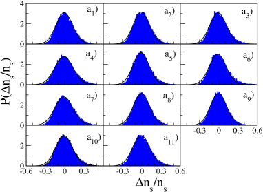
(a)

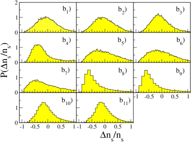
(b)

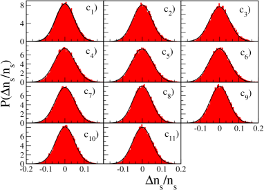
(c)

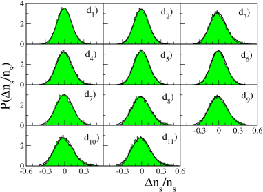
(d)

Figure 4: (Color online) Distributions of relative fluctuations $\Delta n_{s}/n_{s}$, $s=1,...,M=11$: in Fig. 2a, weak perturbation $V=0.1$, high energy, left top panels (blue); in Fig. 2b, weak perturbation $V=0.1$, low energy, right top panels (yellow); in Fig. 2c, strong perturbation $V=0.4$, high energy, left bottom panels (red); in Fig. 2d, strong perturbation $V=0.4$, low energy, right bottom panels (green). Statistics have been obtained by $10^{3}$ different realizations of the random potential and choosing different eigenstates in a small energy window in order to have approximately 20 eigenstates for each realization of the random potential. In all of them, where it is significant (all but the yellow distributions) we superimposed a Gaussian fit (black curve)

These data clearly indicate that for all eigenstates but those in panel b), whose distributions are in the top right panels of Fig. 4, we have that:

• fluctuations are independent of $s$ and therefore statistically independent,

• they are approximately described by Gaussians which is a strong result, in view of the requirement of standard statistical mechanics.

Concerning the eigenstates used in panel b) one can observe that for them one has $d_{loc}\approx 0.2>V=0.1$. Therefore, applying our local criterion for thermal chaotic eigenstates discussed above, we cannot treat them as chaotic eigenstates (in all other cases of course $V>d_{loc}$).

For a more quantitative analysis, for each eigenstate we have computed the corresponding value of $d_{loc}$ as a function of the number of its principal components $N_{pc}$, for the two values of $V$ considered in Fig. 2. The intersections of these points with the horizontal lines $d_{loc}=V$, shown in Fig. 5a) define the critical values $N_{cr}$ indicated by arrows. Then, we expect the fluctuations in the OND to be not statistically acceptable when $N_{pc}<N_{cr}(V)$.

To test such a conjecture we group the eigenstates in small energy windows and calculating in each of them the average fluctuations in OND, $\langle\Delta n_{s}/n_{s}\rangle$. In Fig. 5b) we plot such a quantity vs the renormalized number of principal components $N_{pc}/N_{cr}$. As one can see, for $N_{pc}<N_{cr}$, the average fluctuations $\langle\Delta n_{s}/n_{s}\rangle$ are almost independent of $N_{pc}$, while for $N_{pc}>N_{cr}$ they decay as $1/\sqrt{N_{pc}}$ (dashed line in Fig. 5b ). This gives a strong numerical evidence that for small systems and far from the thermodynamic limit, the value of $N_{pc}$ plays the role of an “effective” number of particles.

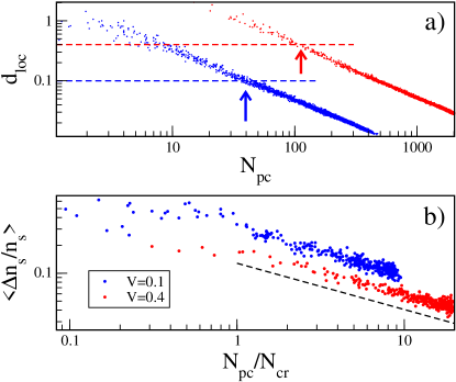
Figure 5: (Color online) Top: $d_{loc}$ as a function of the number of principal components $N_{pc}$ for each eigenstate $\left|\alpha\,\right\rangle$ and two different values of $V$: 0.1 (lower blue points), 0.4 (upper red points). Dashed horizontal lines represent $d_{loc}=V$. Arrows define the critical values $N_{cr}$. Bottom : average relative fluctuations in OND, $\langle\Delta n_{s}/n_{s}\rangle$ vs $N_{pc}/N_{cr}$ for two different $V$ values as indicated in the legend. Dashed line is drawn to guide the eye and stands for for $2/\sqrt{N_{pc}}$. Average fluctuations in OND have been obtained by averaging over 20 close eigenenergies.

V Conclusions

We have shown that the standard Bose-Einstein distribution, known to appear for an ideal gas in the thermodynamic limit, emerges on the level of an individual eigenstate in an isolated system with a finite number of particles. This happens when the inter-particle interaction is strong enough to lead to the onset of chaotic many-body eigenstates in the basis defined by the chosen single-particle spectrum. In our approach we gave an analytical threshold dependent on the eigenstates energy in order to have chaotic eigenstates. For those “thermal eigenstates” we computed the correspondent occupation number distribution and verified that they can be successfully described by a Bose-Einstein distribution with a suitable “dressed“ energy dependent on the inter-particle interaction. We also gave an analytical estimate for the dressed energy well confirmed by direct numerical data.

Special attention has been paid to the fluctuations of occupation numbers. We stress that in order to have the correspondence with the conventional statistical mechanics, fluctuations should be small, independent and Gaussian. Specifically, they decrease as the square root of the number of principal components in chaotic eigenstates. Therefore, for finite isolated systems that are far from the thermodynamic limit, the control parameter for the onset of thermalization is not the number of particles but the number $N_{pc}$ of principal components in chaotic eigenstates. Our analytical findings are complemented by numerical data.

Appendix A Occupation number distribution for a single eigenstate

It is important to observe that the occupation number distribution can be obtained for a single eigenstate, as claimed in the title. The use of averaging over disorder or over close eigenstates, made in the main text, had the only purpose to introduce and analyze statistical errors. Examples of OND for four different eigenstates, for the same parameters and energy regions of those in Fig. 2, are shown in Fig. 6.

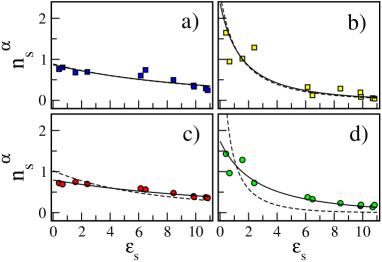
Figure 6: (Color online) Occupation numbers for a single eigenstate $n_{s}^{\alpha}$ for weak ($V=0.1$, top panels) and strong ($V=0.4$, bottom panels) perturbation and different energies: middle of the energy spectrum : a) $E^{\alpha}=28.51$, c) $E^{\alpha}=25.93$; edges : b) $E^{\alpha}=11.27$ and d) $E^{\alpha}=6.05$. Dashed curves are obtained from the BED with $E=E^{\alpha}$ in Eq. (10). Full curves correspond to the BED with the energy $E^{dres}$ in Eq. (12).

Appendix B Properties of F-functions and density of states

Let us start with the conventions used in the definitions of unperturbed ($H_{0}$) and perturbed $(H=H_{0}+V)$ Hamiltonian

$$\begin{array}[]{lll}H_{0}|k\rangle&=E^{0}_{k}|k\rangle\\ &\\ H|\alpha\rangle&=E^{\alpha}|\alpha\rangle,\end{array}$$ (22)

and the change of representation,

$$\left|\alpha\,\right\rangle=\sum_{k}C_{k}^{\alpha}\left|k\,\right\rangle.$$ (23)

The F-function, and the strength function , defined as

$$F^{\alpha}(E)=\sum_{k}|C_{k}^{\alpha}|^{2}\delta(E-E^{0}_{k}),$$ (24)

and

$$F_{k}(E)=\sum_{\alpha}|C^{\alpha}_{k}|^{2}\delta(E-E^{\alpha}),$$ (25)

satisfy many relations, well known in literature (see for instance Ref.our2016 ) and reported here for the reader convenience. First of all they are both normalized,

$$\int\ dE\ F^{\alpha}(E)=\int\ dE\ F_{k}(E)=1.$$ (26)

Introducing the total density of states (DOS):

$$\rho(E)=\sum_{\alpha}\delta(E-E^{\alpha})$$ (27)

and the unperturbed one

$$\rho_{0}(E)=\sum_{k}\delta(E-E^{0}_{k}),$$ (28)

both normalized to the dimension of the Hilbert space $N_{H}$

$$\int\ dE\ \rho_{0}(E)=\int\ dE\ \rho_{0}(E)=N_{H},$$ (29)

it is possible to write :

$$F^{\alpha}(E)\simeq\rho_{0}(E)\langle|C_{k}^{\alpha}|^{2}\rangle_{E^{0}_{k}=E}$$ (30)

where the average is performed over a number of unperturbed eigenstates with energy close to $E$. In the same way, we have

$$F_{k}(E)\simeq\rho(E)\langle|C_{k}^{\alpha}|^{2}\rangle_{E^{\alpha}=E}$$ (31)

where the average is performed over a number of eigenstates with energy close to $E$. Note that instead of averaging over a number of eigenstates, one can use the average inside an individual eigenstate with the ”window moving” method, provided this eigenstate has many uncorrelated components.

The two-body random interaction potential $V$ is assumed to be non-effective on the diagonal, i.e.

$$\langle k|V|k\rangle=0.$$

From these simple relations we can get various results concerning the moments of the distributions.

B.1 First moment of the SF

The following equalities holds,

$$\begin{array}[]{lll}\langle E\rangle_{k}&=\sum_{\alpha}E^{\alpha}|C_{k}^{\alpha}|^{2}=\sum_{\alpha}E^{\alpha}\langle k|\alpha\rangle\langle\alpha|k\rangle&\\ &\\ &=\langle k|H|k\rangle=H_{kk}=\langle k|H_{0}|k\rangle=E^{0}_{k}\\ \end{array}$$ (32)

B.2 Second moment of the SF

$$\begin{array}[]{lll}(\Delta E_{k})^{2}&=\sum_{\alpha}(E^{\alpha}-\langle E\rangle_{k})^{2}|C_{k}^{\alpha}|^{2}\\ &\\ &=\sum_{\alpha}(E^{\alpha})^{2}\langle k|\alpha\rangle\langle\alpha|k\rangle-\langle E\rangle_{k}^{2}\\ &\\ &=\langle k|H^{2}|k\rangle-(H_{kk})^{2}\\ &\\ &=\sum_{j}\langle k|H|j\rangle\langle j|H|k\rangle-(H_{kk})^{2}\\ &\\ &=\sum_{j\neq k}H_{kj}^{2}\end{array}$$ (33)

B.3 First moment (center) of the perturbed and unperturbed spectrum (DOS)

Let us define $E_{c}$ the center of the perturbed spectrum and $E_{c}^{0}$ the center of the unperturbed one. It is easy to see that in our model they coincide. Indeed,

$$\begin{array}[]{lll}\mkern 1.5mu\overline{\mkern-1.5muE\mkern-1.5mu}&=E_{c}=\frac{1}{N_{H}}\sum_{\alpha}E^{\alpha}=\frac{1}{N_{H}}Tr[H]=\frac{1}{N_{H}}\sum_{k}\langle k|H|k\rangle\\ &\\ &=\frac{1}{N_{H}}\sum_{k}\langle k|H_{0}|k\rangle=\frac{1}{N_{H}}\sum_{k}E^{0}_{k}=E_{c}^{0}\\ \end{array}$$ (34)

B.4 Second moment of the DOS

$$\begin{array}[]{lll}\mkern 1.5mu\overline{\mkern-1.5muE^{2}\mkern-1.5mu}&=\frac{1}{N_{H}}\sum_{\alpha}E_{\alpha}^{2}=\frac{1}{N_{H}}Tr[H^{2}]=\frac{1}{N_{H}}\sum_{k}\langle k|H^{2}|k\rangle\\ &\\ &=\frac{1}{N_{H}}\sum_{k}\sum_{j}\langle k|H|j\rangle\langle j|H|k\rangle\\ &\\ &=\frac{1}{N_{H}}\sum_{k}H_{kk}^{2}+\frac{1}{N_{H}}\sum_{k}\sum_{j\neq k}H_{kj}^{2}\end{array}$$ (35)

B.5 Relation between second moments of the DOS

Let us define $\sigma_{E}^{2}$ and $\sigma_{0}^{2}$ the variances of the perturbed and unperturbed DOS. Then, the following relation hold,

$$\begin{array}[]{lll}\sigma_{E}^{2}&=\mkern 1.5mu\overline{\mkern-1.5muE^{2}\mkern-1.5mu}\mkern 1.5mu-\mkern 1.5mu\overline{\mkern-1.5muE\mkern-1.5mu}\mkern 1.5mu^{2}=\frac{1}{N_{H}}\sum_{k}H_{kk}^{2}+\frac{1}{N_{H}}\sum_{k}\sum_{j\neq k}H_{kj}^{2}\\ &\\ &-(E_{c}^{0})^{2}=\frac{1}{N_{H}}\sum_{k}(E^{0}_{k})^{2}-\left(\frac{1}{N_{H}}\sum_{k}E^{0}_{k}\right)^{2}+\\ &\\ &\frac{1}{N_{H}}\sum_{j\neq k}(\Delta E_{k})^{2}\equiv\sigma_{0}^{2}+\mkern 1.5mu\overline{\mkern-1.5mu(\Delta E)^{2}\mkern-1.5mu}\end{array}$$ (36)

where in the latter equality we have defined $\mkern 1.5mu\overline{\mkern-1.5mu(\Delta E)^{2}\mkern-1.5mu}\mkern 1.5mu$ as the average of the variances of all SF (each SF is defined for any given basis state $|k\rangle$).

References

- (1) V. Zelevinsky, M. Horoi, and B.A. Brown, Phys. Lett. B 350, (1995) 141; M. Horoi, V. Zelevinsky, and B.A. Brown, Phys. Rev. Lett. 74, (1995) 5194; V. Zelevinsky, B.A. Brown, M. Horoi and N. Frazier, Phys. Rep. 276, (1996) 85; V. Zelevinsky, Ann. Rev. Nucl. Part. Sci. 46, (1996) 237.
- (2) V. V. Flambaum, A. A. Gribakina, G. F. Gribakin, M. G. Kozlov, Phys. Rev. A 50 (1994) 267; G. F. Gribakin, A. A. Gribakina, and V. V. Flambaum, Aust. J. Phys. 52 (1999) 443.
- (3) V.V. Flambaum, F.M. Izrailev, and G. Casati, Phys. Rev. E 54, (1996) 2136; V.V. Flambaum, F.M. Izrailev, Phys. Rev. E 55 (1997) R13.
- (4) V.V. Flambaum and F.M. Izrailev, Phys. Rev. E 56, (1997) 5144.
- (5) J.M. Deutsch, Phys. Rev. A 43, (1991) 2046; M. Srednicki, Phys. Rev. E 50, (1994) 888; M. Rigol, V. Dunjko, and M. Olshanii, Nature 452, (2008) 854; A. Polkovnikov, K. Sengupta, A. Silva, and M. Vengalattore, Rev. Mod. Phys. 83, (2011) 863; L. D’Alessio, Y. Kafri, A. Polkovnikov, and M. Rigol, Advances in Physics, 65, (2016) 239-362.
- (6) M. Greiner, O. Mandel, T.W. Hansch, and I. Bloch, Nature 419, (2002) 51; T. Kinoshita, T. Wenger, and D.S. Weiss, Nature 440, (2006) 900; S. Trotzky et. al., Nature Phys. 8, (2012) 325; M. Gring, et al. Science 337, (2012) 1318; A.M. Kaufman et al. Science, 353 (2016), 794-800.
- (7) J. Smith et al., Nature Phys. 12, (2016) 907–911.
- (8) V. K. B. Kota, A. Relano, J. Retamosa, and M. Vyas, Jour. of Stat. Mech.: Theory and Experiment 2011, (2011) P10028.
- (9) L.F. Santos, F. Borgonovi, and F.M. Izrailev, Phys. Rev. Lett. 108, (2012) 094102; Phys. Rev. E. 85, (2012) 036209 .
- (10) E. J. Torres-Herrera and Lea F. Santos, Phys. Rev E, 88, (2013) 042121
- (11) F. Borgonovi, F.M. Izrailev, L.F. Santos, and V.G. Zelevinsky, Phys. Rep. 626 (2016) 1.
- (12) J. B. French and S. S. M. Wong, Phys. Lett. B 35 , 5 (1970); O. Bohigas and J. Flores, Phys. Lett. B 34, 261 (1971)
- (13) L.D. Landau and E.M. Lifshitz, Statistical Physics, Pergamon Press, Oxford, 1958.
- (14) R. V. Jensen and R. Shankar, Phys. Rev. Lett. 54, 1879 (1985).
- (15) G.P. Berman, F. Borgonovi, F.M. Izrailev, A. Smerzi, Phys. Rev. Lett. 92, (2004) 030404.
- (16) O. Bohigas and J. Flores, Phys. Lett. B 34, (1971) 261; 35 (1971) 383; J.B. French and S.S.M. Wong, Phys. Lett. B 33 (1970) 449; 35 (1971) 5.
- (17) T.A. Brody, et al. Rev. Mod. Phys 53, (1981) 385; V.K.B. Kota, Phys. Rep. 347 (2001) 223; H.A. Weidenmuller and G.E. Mitchell, Rev. Mod. Phys. 81 (2009) 539; B.L. Altshuler, Y. Gefen, A. Kamenev, L.S. Levitov, Phys. Rev. Lett. 78 (1997) 2803, V. K. B. Kota, Embedded Random Matrix Ensembles in Quantum Physics, Lecture Notes in Physics, Vol. 884, Springer (2014).
- (18) L. Benet and H.A. Weidenmuller, J. of Phys. A: Math. and Gen., 36, (2003) 3569.
- (19) N.D. Chavda, V.K.B. Kota, V. Potbhare, Phys. Lett. A, 376, (2012) 2972, N. D. Chavda, V. K. B. Kota, ANNALEN DER PHYSIK (2017), 1600287.
- (20) A. Bohr and B. R. Mottelson, Nuclear Structure, Benjamin, New York, 1969.
- (21) E. J. Torres-Herrera and Lea F. Santos, New J. Phys. 16, 063010 (2014)
- (22) P.R. Levstein, G. Usaj, H.M. Pastawski, The Jour. of Chem. Phys. 108, (1998) 2718; G. Usaj, H.M. Pastawski, P.R. Levstein, Molecular Physics, 95, (1998) 1229.
- (23) G. Casati, B.V. Chirikov, I. Guarneri, F.M. Izrailev, Phys. Rev. E 48 (1993) R1613; Phys. Lett. A 223 (1996) 430.
- (24) R. Nandkishore and D.A. Huse, Annual Review of Condensed Matter Physics 6 (2015) 15.
- (25) Y.B.Rumer and M.S.Ryvkin, Thermodynamics, Statistical Physics, and Kinetics (Mir, Moskow, 1980).
- (26) C.Tian, K.Yang, and J.Wang, ArXiv 1606.08371v1 (2016).
- (27) F. Borgonovi, I. Guarneri, and F.M. Izrailev, Phys. Rev. E. 57, (1998) 5291; F. Borgonovi, I. Guarneri, F.M. Izrailev, and G. Casati, Phys. Lett. A 247, (1998) 140.