Enumerations, Forbidden Subgraph Characterizations,
and the Split-Decomposition

Abstract

Forbidden characterizations may sometimes be the most natural way to describe families of graphs, and yet these characterizations are usually very hard to exploit for enumerative purposes.

By building on the work of Gioan and Paul (2012) and Chauve et al. (2014), we show a methodology by which we constrain a split-decomposition tree to avoid certain patterns, thereby avoiding the corresponding induced subgraphs in the original graph.

We thus provide the grammars and full enumeration for a wide set of graph classes: ptolemaic, block, and variants of cactus graphs (2,3-cacti, 3-cacti and 4-cacti). In certain cases, no enumeration was known (ptolemaic, 4-cacti); in other cases, although the enumerations were known, an abundant potential is unlocked by the grammars we provide (in terms of asymptotic analysis, random generation, and parameter analyses, etc.).

We believe this methodology here shows its potential; the natural next step to develop its reach would be to study split-decomposition trees which contain certain prime nodes. This will be the object of future work.

Introduction

Many important families of graphs can be defined (sometimes exclusively) through a forbidden graph characterization. These characterizations exist in several flavors:

1. Forbidden minors, in which we try to avoid certain subgraphs from appearing after arbitrary edge contractions and vertex deletion.

2. Forbidden subgraphs, in which we try to avoid certain subgraphs from appearing as subsets of the vertices and edges of a graph.

3. Forbidden induced subgraphs, in which we try to avoid certain induced subgraphs from appearing (that is we pick a subset of vertices, and use all edges with both endpoints in that subset).

As far as we know, while these notions are part and parcel of the work of graph theorists, they are usually not exploited by analytic combinatorists. For forbidden minors, there is the penetrating article of Bousquet-Mélou and Weller [BoWe14]. For forbidden subgraphs or forbidden induced subgraphs, we know of few papers, except because of the simple nature of graphs [RaTh01], or because some other, alternate property is used instead [CaWo03], or only asymptotics are determined [RaTh04].

We are concerned, in this paper, with forbidden induced subgraphs.

Split-decomposition and forbidden induced subgraphs.

Chauve et al. [ChFuLu14] observed that relatively well-known graph decomposition, called the split-decomposition, could be a fruitful means to enumerate a certain class called distance-hereditary graphs, of which the enumeration had until then not been known (since the best known result was the bound from Nakano et al. [NaUeUn09], which stated that there are at most $\cramped{2^{\lfloor 3.59n\rfloor}}$ unlabeled distance-hereditary graphs on $n$ vertices).

In addition, the reformulated version of this split-decomposition introduced by Paul and Gioan, with internal graph labels, considerably improved the legibility of the split-decomposition tree.

We have discovered, and we try to showcase in this paper, that the split-decomposition is a very convenient tool by which to find induced subpatterns: although various connected portions of the graphs may be broken down into far apart blocks in the split-decomposition tree, the property that there is an alternated path between any two vertices that are connected in the original graph is very powerful, and as we show in Section 2 of this paper, allows to deduce constraints following the appearance of an induced pattern or subgraph.

Outline of paper.

In Section 1, we introduce all the definitions and preliminary notions that we need for this paper to be relatively self-contained (although it is based heavily in work introduced by Chauve et al. [ChFuLu14]).

In Section 2, we introduced a collection of bijective lemmas, which translate several forbidden patterns (a cycle with 4 vertices, a diamond, cliques, a pendant vertex and a bridge, all illustrated in Figure 4) into constraints on the split-decomposition tree of a graph. In each of the subsequent setions, we show how these constraints can be used to express a formal symbolic grammar that describes the constrained tree—and by so doing, we obtain grammar for the associated class of graphs.

We start by studying block graphs in Section 3, because their structure is sufficiently constrained as to yield a relatively simple grammar. We then study ptolemaic graphs in Section 4 (which allows us to showcase how to use the symbolic grammar to save “state” information, since we have to remember the provenance of the hierarchy of each node to determine whether it has a center as a starting point). And we finally look at some varieties of cactus graphs in Section 5.

Finally, in Section 6, we conclude and introduce possible future directions in which to continue this work.

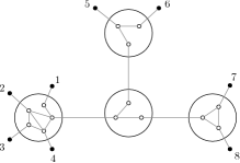
(a) A graph-labeled tree.

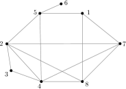
(b) Original graph for (or accessibility graph of) the graph-labeled tree in Figure 1.

Figure 1: Two leaves of the split-decomposition graph-labeled tree (left) correspond to adjacent vertices in the original graph that was decomposed (right) if there exists an alternated path: a path between those leaves, which uses at most one interior edge of any given graph label. For example, vertex 5 is adjacent to vertex 4 in the original graph, because there is an alternated path between the two corresponding leaves in the split-decomposition tree; vertex 5 is not adjacent to vertex 3 however, because that would require the path to take two interior edges of the (prime) leftmost graph-label.

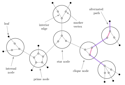
Figure 2: In this figure, we present a few terms that we use a lot in this article.

(a) Example of a star-join.

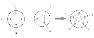
(b) Example of a clique-join.

Figure 3: The star-join and clique-join operations result in the merging of two internal nodes of a split-decomposition tree. A split-decomposition tree in which neither one of these operations may be applied (and in which all non-clique and non-star nodes are prime nodes) is said to be reduced.

1 Definitions and Preliminaries

In this rather large section, we introduce standard definitions from graph theory (1.1 to 1.3) and analytic combinatorics (1.4), and then present a summary of the work of Chauve et al. [ChFuLu14] (1.5), as well as summary of how they used the dissymmetry theorem, introduced by Bergeron et al. [BeLaLe98] (1.6).

1.1 Graph definitions.

For a graph $G$, we denote by $V(G)$ its vertex set and $E(G)$ its edge set. Moreover, for a vertex $x$ of a graph $G$, we denote by $N(x)$ the neighbourhood of $x$, that is the set of vertices $y$ such that $\{x,y\}\in E(G)$; this notion extends naturally to vertex sets: if $\cramped{V_{1}}\subseteq V(G)$, then $N(\cramped{V_{1}})$ is the set of vertices defined by the (non-disjoint) union of the neighbourhoods of the vertices in $\cramped{V_{1}}$. Finally, the subgraph of $G$ induced by a subset $\cramped{V_{1}}$ of vertices is denoted by $G[\cramped{V_{1}}]$.

Given a graph $G$ and vertices $(u,v)\in\cramped{V(G)^{2}}$ in the same connected component of $G$, the distance between $u$ and $v$ denoted by $\cramped{d_{G}}(u,v)$ is defined as the length of the shortest path between $u$ and $v$.

A graph on $n$ vertices is labeled if its vertices are identified with the set $\{1,\dots,$ $n\}$, with no two vertices having the same label. A graph is unlabeled if its vertices are indistinguishable.

A clique on $k$ vertices, denoted $\cramped{K_{k}}$ is the complete graph on $k$ vertices (i.e., there exists an edge between every pair of vertices). A star on $k$ vertices, denoted $\cramped{S_{k}}$, is the graph with one vertex of degree $k-1$ (the center of the star) and $k-1$ vertices of degree $1$ (the extremities of the star).

1.2 Special graph classes.

The following two graph classes are important because they are supersets of the classes we study in this paper.

Definition 1.1.

A connected graph $G$ is distance-hereditary if for every induced subgraph $H$ and every $(u,v)\in\cramped{V(H)^{2}}$, $\cramped{d_{G}}(u,v)=\cramped{d_{H}}(u,v)$.

Definition 1.2.

A connected graph is chordal, or triangulated, or $\cramped{C_{\geqslant 4}}$-free, if every cycle of length at least 4 has a chord.

1.3 Split-decomposition.

We first introduce the notion of graph-labeled tree, due to Gioan and Paul [GiPa12], then define the split-decomposition and finally give the characterization of a reduced split-decomposition tree, described as a graph-labeled tree.

Definition 1.3.

A graph-labeled tree $(T,\cls{F})$ is a tree $T$ in which every internal node $v$ of degree $k$ is labeled by a graph $\cramped{G_{v}}\in\cls{F}$ on $k$ vertices, called marker vertices, such that there is a bijection $\cramped{\rho_{v}}$ from the edges of $T$ incident to $v$ to the vertices of $\cramped{G_{v}}$.

For example, in Figure 1 the internal nodes of $T$ are denoted with large circles, the marker vertices are denoted with small hollow circles, the leaves of $T$ are denoted with small solid circles, and the bijection $\cramped{\rho_{v}}$ is denoted by each edge that crosses the boundary of an internal node and ends at a marker vertex.

Importantly, the graph labels of these internal nodes are for convenience alone—indeed the split-decomposition tree itself is unlabeled. However as we will see in this paper, these graph-labeled trees are a powerful tool by which to look at the structure of the original graph they describe. Some elements of terminology have been summarized in Figure 2, as these are frequently referenced in the proofs of Section 2.

Definition 1.4.

Let $(T,\cls{F})$ be a graph-labeled tree and let $\ell,\ell^{\prime}\in V(T)$ be leaves of $T$. We say that there is an alternated path between $\ell$ and $\ell^{\prime}$, if there exists a path from $\ell$ to $\ell^{\prime}$ in $T$ such that for any adjacent edges $e=(u,v,$) and $e^{\prime}=(v,w,$) on the path, $(\cramped{\rho_{v}}(e),\cramped{\rho_{v}}(e^{\prime}),\in)E(\cramped{G_{v}})$.

Definition 1.5.

The original graph, also called accessibility graph, of a graph-labeled tree $(T,\cls{F})$ is the graph $G=G(T,\cls{F})$ where $V(G)$ is the leaf set of $T$ and, for $x,y\in V(G)$, $(x,y)\in E(G)$ iff $x$ and $y$ are accessible in $(T,\cls{F})$.

Figures 1 and 2 illustrate the concept of alternated path: it is, more informally, a path that only ever uses at most one interior edge of graph-label.

Definition 1.6.

A split [Cunningham82] of a graph $G$ with vertex set $V$ is a bipartition $(\cramped{V_{1}},\cramped{V_{2}})$ of $V$ (i.e., $V=\cramped{V_{1}}\cup V_{2}$, $\cramped{V_{1}}\cap\cramped{V_{2}}=\emptyset$) such that

1. $|V_{1}|\geqslant 2$ and $|V_{2}|\geqslant 2$;

2. every vertex of $N(V_{1})$ is adjacent to every of $N(V_{2})$.

A graph without any split is called a prime graph. A graph is degenerate if any partition of its vertices without a singleton part is a split: cliques and stars are the only such graphs.

Informally, the split-decomposition of a graph $G$ consists in finding a split $(\cramped{V_{1}},\cramped{V_{2}})$ in $G$, followed by decomposing $G$ into two graphs $\cramped{G_{1}}=G[\cramped{V_{1}}\cup\{\cramped{x_{1}}\}]$ where $\cramped{x_{1}}\in N(\cramped{V_{1}})$ and $\cramped{G_{2}}=G[\cramped{V_{2}}\cup\{\cramped{x_{2}}\}]$ where $\cramped{x_{1}}\in N(\cramped{V_{2}})$ and then recursively decomposing $\cramped{G_{1}}$ and $\cramped{G_{2}}$. This decomposition naturally defines an unrooted tree structure of which the internal vertices are labeled by degenerate or prime graphs and whose leaves are in bijection with the vertices of $G$, called a split-decomposition tree. A split-decomposition tree $(T,\mathcal{F})$ with $\mathcal{F}$ containing only cliques with at least three vertices and stars with at least three vertices is called a clique-star tree

It can be shown that the split-decomposition tree of a graph might not be unique (i.e., several sequences of decompositions of a given graph can lead to different split-decomposition trees), but following Cunningham [Cunningham82], we obtain the following uniqueness result, reformulated in terms of graph-labeled trees by Gioan and Paul [GiPa12].

[Cunningham [Cunningham82]]For every connected graph $G$, there exists a unique split-decomposition tree such that:

1. every non-leaf node has degree at least three;

2. no tree edge links two vertices with clique labels;

3. no tree edge links the center of a star-node to the extremity of another star-node.

Such a tree is called reduced, and this theorem establishes a one-to-one correspondence between graphs and their reduced split-decomposition trees. So enumerating the split-decomposition trees of a graph class provides an enumeration for the corresponding graph class, and we rely on this property in the following sections.

Figure 3 demonstrates the star-join and clique-join operations which respectively allow trees that do not verify conditions (b) and (c) to be further reduced—in terms of number of internal nodes.

Lemma 1.7 (Split-decomposition tree characterization of distance-hereditary graphs [Cunningham82, GiPa12]).

A graph is distance-hereditary if and only its split-decomposition tree is a clique-star tree. For this reason, distance-hereditary graphs are called totally decomposable with respect to the split-decomposition.

1.4 Decomposable structures.

In order to enumerate classes of split-decomposition trees, we use the framework of decomposable structures, described by Flajolet and Sedgewick [FlSe09]. We refer the reader to this book for details and outline below the basic idea.

We denote by $\clsAtom$ the combinatorial family composed of a single object of size $1$, usually called atom (in our case, these refer to a leaf of a split-decomposition tree, i.e., a vertex of the corresponding graph).

Given two disjoint families $\cls{A}$ and $\cls{B}$ of combinatorial objects, we denote by $\cls{A}+\cls{B}$ the disjoint union of the two families and by $\cls{A}\times\cls{B}$ the Cartesian product of the two families.

Finally, we denote by $\Set{\cls{A}}$ (resp. $\cramped{\Set[\geqslant k]{\cls{A}}}$, $\cramped{\Set[k]{\cls{A}}}$) the family defined as all sets (resp. sets of size at least $k$, sets of size exactly $k$) of objects from ${\cls{A}}$, and by $\cramped{\Seq[\geqslant k]{\cls{A}}}$, the family defined as all sequences of at least $k$ objects from ${\cls{A}}$.

1.5 Split-decomposition trees expressed symbolically.

While approaching graph enumeration from the perspective of tree decomposition is not a new idea (the recursively decomposable nature of trees makes them well suited to enumeration), Chauve et al. [ChFuLu14] brought specific focus to Cunningham’s split-decomposition.

Their way of describing constrained split-decomposition trees with decomposable grammars is the starting point of this paper, so we briefly outline their method here.

Example

Let us consider the split-decomposition tree of Figure 1, and illustrate how this tree can be expressed recursively as a rooted tree.

Suppose the tree is rooted at vertex 5. Assigning a root immediately defines a direction for all tree edges, which can be thought of as oriented away from the root. Starting from the root, we can set out to traverse the tree in the direction of the edges, one internal node at a time.

We start at the root, vertex 5. The first internal node we encounter is a star-node, and since we are entering it from the star’s center, we have to describe what is on each of its two remaining extremities. On one of the extremities there is a leaf, 6; on the other, there is another split-decomposition subtree, of which the first internal node we encounter happens to be another star-node.

This time, we enter the star-node through one of its extremity. So we must describe what is connected to its center and its remaining extremities (of which there is only one).

Both of these are connected to smaller split-decomposition trees: the extremity is connected itself to a clique-node, which we enter through one of its undistinguished edges (leaving the two other to go to leaves, 7 and 8); the center of the star-node is connected to a prime node, and so on.

Grammar description

Now, to describe this tree symbolically, let’s consider the rule for star-nodes (assuming we are, unlike in the tree of Figure 1, in a clique-star tree that has no prime internal nodes). First assume like at the beginning of our example, that we enter a star-node through its center: we have to describe what the extremities can be connected to.

According to Cunningham’s Theorem: we know that there are at least two extremities (since every non-leaf node has degree at least three); and we know that the star-node’s extremities cannot be connected to the center of another star-node. We call $\cramped{\cls[C]{S}}$ a split-decomposition tree that is traversed starting at a star-node entered through its center. We have

$$\cls[C]{S}=\Set[\geqslant 2]{\clsAtom+\cls{K}+\cls[X]{S}}$$

because indeed, we have at least two extremities, which are not ordered—so $\cramped{\Set[\geqslant 2]{\ldots}}$—and each of these extremities can either lead to a leaf, $\clsAtom$, a clique-node entered through any edge, $\cls{K}$, and a star-node entered through one of its extremities, $\cramped{\cls[X]{S}}$.

For a star-node entered through its extremity, we have a similar definition, with a twist,

$$\cls[X]{S} =\left(\clsAtom+\cls{K}+\cls[C]{S}\right)\times\Set[\geqslant 1]{\clsAtom+\cls{K}+\cls[X]{S}}$$

because the center—which can lead to a leaf, $\clsAtom$, a clique-node, $\cls{K}$, or a star-node entered through its center, $\cramped{\cls[C]{S}}$—is distinct from the extremities (which, from the perspective of the star-node itself, are undistinguishable). We thus express the subtree connected through the center as separate from those connected through the extremities: this is the reason for the Cartesian product (rather than strictly using non-ordered constructions such as $\Set$).

Conventions

As explained above, we use rather similar notations to describe the combinatorial classes that arise from decomposing split-decomposition trees. These notations are summarized in Table LABEL:tab:symbols, and the most frequently used are:

• $\cls{K}$ is a clique-node entered through one of its edges;

• $\cramped{\cls[C]{S}}$ is a star-node entered through its center;

• $\cramped{\cls[X]{S}}$ is a star-node entered through one of its extremities.

Furthermore because we provide grammars for tree classes that are both rooted and unrooted, we use some notation for clarity. In particular, we use $\cramped{\clsAtom_{\bullet}}$ to denote the rooted vertex, although this object does not differ in any way from any other atom $\clsAtom$.

Terminology

In the rest of this paper, we describe the combinatorial class $\cramped{\cls[X]{S}}$ as representing a “a star-node entered through an extremity”, but others may have alternate descriptions: such as “a star-node linked to its parent by an extremity”; or such as Iriza [Iriza15], “a star-node with the subtree incident to one of its extremities having been removed”—all these descriptions are equivalent (but follow different viewpoints).

1.6 The dissymmetry theorem.

All the grammars produced by this methodology are rooted grammars: the trees are described as starting at a root, and branching out to leaves—yet the split-decomposition trees are not rooted, since they decompose graphs which are themselves not rooted.

If we were limiting ourselves to labeled objects, it would be simple to move from a rooted object to an unrooted one, because there are exactly $n$ ways to root a tree with $n$ labeled leaves. But because we allow the graphs (and associated split-decomposition trees) to be unlabeled, some symmetries make the transition to unrooted objects less straightforward.

While this problem has received considerable attention since Pólya [Polya37, PoRe87], Otter [Otter48] and others [HaUh53], we choose to follow the lead of Chauve et al. [ChFuLu14], and appeal to a more recent result, the dissymmetry theorem. This theorem was introduced by Bergeron et al. [BeLaLe98] in terms of ordered and unordered pairs of trees, and was eventually reformulated in a more elegant manner, for instance by Flajolet and Sedgewick [FlSe09, VII.26 p. 481] or Chapuy et al. [ChFuKaSh08, §3]. It states

$$\cls{A}+{\cls{A}}_{\circ\rightarrow\circ}\simeq{\cls{A}}_{\circ}+{\cls{A}}_{\circ-\circ}$$ (1)

where $\cls{A}$ is the unrooted class of trees, and $\cramped{{\cls{A}}_{\circ}}$, $\cramped{{\cls{A}}_{\circ-\circ}}$, $\cramped{{\cls{A}}_{\circ\rightarrow\circ}}$ are the rooted classes of trees respectively where only the root is distinguished, an edge from the root is distinguished, and a directed, outgoing edge from the root is distinguished. The proof is straightforward, see Drmota [HoECDrmota15, §4.3.3, p. 293], and involves the notion of center of a tree.

(a) A $\cramped{C_{4}}$ (cycle with 4 vertices).

(b) A diamond.

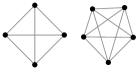
(c) Cliques (here, of size 4 and 5).

(d) A pendant vertex.

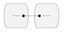
(e) A bridge.

Figure 4: These are the induced forbidden subgraphs that we investigate in this paper. In Section 2, we introduce a series of lemmas that characterize the split-decomposition tree of a (totally decomposable) graph which avoids one or some of these induced subgraphs.

For more details on the dissymmetry theorem, see Chauve et al. [ChFuLu14, §2.2 and §3]. We will content ourselves with some summary remarks:

• The process of applying the dissymmetry theorem involves rerooting the trees described by a grammar in every possible way. Indeed, the trees obtained from our methodology will initially be rooted at their leaves. For the dissymmetry theorem, we re-express the grammar of the tree in all possible ways it can be rooted.

• A particularity of the dissymmetry theorem is that in this rerooting process, we can completely ignore leaves [ChFuLu14, Lemma 1], as the effect of doing this cancels out in the subtraction of Eq. (1):

  Lemma 1.8 (Dissymmetry theorem leaf-invariance [ChFuLu14]).

  In the dissymmetry theorem for trees, when rerooting at the nodes (or atoms) of a combinatorial tree-like class $\cls{A}$, leaves can be ignored.

• In terms of notation, we systematically refer to $\cls[\omega]{T}$ as trees re-rooted in a node (or edge) of type $\omega$. Often these rerooted trees present the distinct characteristic that, unlike the trees described in the rooted grammars, they are not “missing a subtree.” Thus the combinatorial class $\cramped{\cls[S]{T}}$ refers to a split-decomposition tree (of some graph family) that is rerooted at star-nodes: in this context, we must account both for the center, and at least two extremities.

• This is a relatively simple theorem to apply; the downside is that it only yields an equality of the coefficient, but it loses the symbolic meaning of a grammar. This is a problem when using the tools of analytic combinatorics [FlSe09], in particular those having to do with random generation [FlZiVa94, DuFlLoSc04, FlFuPi07].

• An alternate tool to unroot combinatorial classes, cycle-pointing [BoFuKaVi11], does not have this issue: it is a combinatorial operation (rather than algebraic one), and it allows for the creation of random samplers for a class. However it is more complex to use, though Iriza [Iriza15] has already applied it to the distance-hereditary and 3-leaf power grammars of Chauve et al. [ChFuLu14].

2 Characterization & Forbidden Subgraphs

In this section, we provide a set of bijective lemmas that characterize the split-decomposition tree of a graph that avoids any of the forbidden induced subgraphs of Figure 4.

2.1 Elementary lemmas.

We first provide three simple lemmas, which essentially have to do with the fact that the split-decomposition tree is a tree. Their proofs are provided in Appendix LABEL:app:proof-tree-lemmas, and notably are still valid in the presence of prime nodes (i.e., these elementary lemmas would still apply to a split-decomposition tree that while reduced, is not purely a clique-star tree—even though those are the only trees that we work with in the context of this paper).

Lemma 2.1.

Let $G$ be a totally decomposable graph with the reduced clique-star split-decomposition tree $T$, any maximal alternated path starting from any node in $V(T)$ ends in a leaf.

Lemma 2.2.

Let $G$ be a totally decomposable graph with the reduced clique-star split-decomposition tree $T$ and let $u\in V(T)$ be an internal node. Any two maximal alternated paths $P$ and $Q$ that start at distinct marker vertices of $u$ but contain no interior edges from $\cramped{G_{u}}$ end at distinct leaves.

Lemma 2.3.

Let $G$ be a totally decomposable graph with the reduced clique-star split-decomposition tree $T$. If $T$ has a clique-node of degree $n$, then $G$ has a corresponding induced clique on (at least) $n$ vertices.

2.2 Forbidden subgraphs lemmas

Definition 2.4.

Let $G$ be a totally decomposable graph with the reduced clique-star split-decomposition tree $T$. A center-center path in $T$ is an alternated path $P$, such that the endpoints of $P$ are centers of star-nodes $(u,v)\in\cramped{V(T)^{2}}$ and $P$ does not contain any interior edge of either star-node.

Lemma 2.5 (Split-decomposition tree characterization of $\cramped{C_{4}}$-free graphs).

Let $G$ be a totally decomposable graph with the reduced clique-star split-decomposition tree $T$. $G$ does not have any induced $\cramped{C_{4}}$ if and only if $T$ does not have any center-center paths.

Proof 2.6.

[$\Rightarrow$]  Let $T$ be a clique-star tree with a center-center path $P$ between the centers of two star-nodes $u,v\in V(T)$; we will show that the accessibility graph $G(T)$ has an induced $\cramped{C_{4}}$.

Let $\cramped{c_{u}}\in\cramped{G_{u}}$ and $\cramped{c_{v}}\in\cramped{G_{v}}$ be the endpoints of $P$. Since $T$ is assumed to be a reduced split-decomposition tree (Theorem 1.6), $u$ and $v$ have degree at least three and thus $\cramped{G_{u}}$ and $\cramped{G_{u}}$ have at least two extremities. Therefore, there are at least two maximal alternated paths out of $u$ (resp. $v$), each beginning at an extremity of $\cramped{G_{u}}$ (resp. $\cramped{G_{v}}$) and not using any interior edges of $\cramped{G_{u}}$ (resp. $\cramped{G_{v}}$). By Lemma 2.2, these paths end at distinct leaves $a,b\in V(T)$ (resp. $c,d\in V(T)$), as shown in Figure 5.

Now consider the accessibility graph $G$ of $T$. First, we observe that the pairs $(a,c)$, $(a,d)$, $(b,c)$, $(b,d)$ all belong to the edge set of $G$. We will show this for the edge $(a,c)$ by extending $P$ into an alternated path in $T$ from $a$ to $c$. The argument extends symmetrically to the other three edges.

Let $\cramped{P_{a}}$ be the alternated path between $a$ and an extremity of $\cramped{G_{u}}$, and let $\cramped{P_{c}}$ be the alternated path between $c$ and an extremity of $\cramped{G_{v}}$. To show $(a,c)\in E(G)$, we extend $P$ into the following alternated path:

$$P_{a},c_{u},P,c_{v},P_{c}$$

We next observe that $(a,b)$ and symmetrically $(c,d)$ cannot belong to the edge set of G. Since $T$ is a tree, there is a unique path in $T$ between $a$ and $b$, which passes through $u$. This unique path must use two interior edges within $\cramped{G_{u}}$ and therefore cannot be alternated. Consequently, $(a,b)\not\in E(G)$. It can be shown by a similar argument that $(c,d)\not\in E(G)$. Therefore, the induced subgraph of $G$ consisting of $a,b,c,d$ is a $\cramped{C_{4}}$ illustrated in Figure 5.

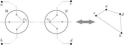
Figure 5: A center-center path in a split-decomposition tree translates to an induced $\cramped{C_{4}}$ in the corresponding accessibility graph, see Lemma 2.5.

[$\Leftarrow$]  Let $G$ be a totally decomposable graph with an induced $\cramped{C_{4}}$ with its vertices arbitrarily labeled $(a,c,b,d)\in V(G)$ as in Figure 5. We will show that the reduced split-decomposition tree $T$ of $G$ has a center-center path.

First, we will show that there is a star-node $v\in V(T)$ that has alternated paths out of its extremities ending in $c$ and $d$. Since $(a,c),(a,d)\in E(G)$, there must exist alternated paths $\cramped{P_{a,c}}$ and $\cramped{P_{a,d}}$, which begin at the leaf $a$ and end at the leaf $c$ or $d$ respectively. Let $v\in V(T)$ be the internal node that both $\cramped{P_{a,c}}$ and $\cramped{P_{a,d}}$ enter via the same edge $\cramped{\rho_{c_{v}}}$ but exit via different edges $\cramped{\rho_{x_{c}}}$ and $\cramped{\rho_{x_{d}}}$ respectively. We claim that $v$ must be a star-node, such that $\cramped{c_{v}}$ is its center and $\cramped{x_{c}}$ and $\cramped{x_{d}}$ are two of its extremities. It is sufficient to show $(\cramped{x_{c}},\cramped{x_{d}})\not\in E(\cramped{G_{v}})$, which is indeed true because otherwise, we could use that edge and the disjoint parts of $\cramped{P_{a,c}}$ and $\cramped{P_{a,d}}$ to construct the alternated path between $c$ and $d$, contradicting the fact that $(c,d)\not\in E(G)$.

Next, we will show that there is a star-node $u\in V(T)$ that has alternated paths out of its extremities ending in $a$ and $b$ and forms a center-center path with $v$. Consider this time the alternated path $\cramped{P_{b,c}}$ between leaves $b$ and $c$, as well as $\cramped{P_{a,c}}$ defined above. Similar to the argument above, let $u\in V(T)$ be the internal node that both $\cramped{P_{a,c}}$ and $\cramped{P_{b,c}}$ enter via the same edge $\cramped{\rho_{c_{u}}}$ but exit via different edges $\cramped{\rho_{x_{a}}}$ and $\cramped{\rho_{x_{b}}}$ respectively. With the same argument outlined above, $u$ must be a star-node, such that $\cramped{c_{u}}$ is its center and $\cramped{x_{a}}$ and $\cramped{x_{b}}$ are two of its extremities. It remains to show that $u$ and $v$ form a center-center path.

Suppose $u$ and $v$ do not form a center-center path. Then $u$ must be on the common part of $\cramped{P_{a,c}}$ and $\cramped{P_{b,c}}$ between $\cramped{x_{c}}$ and $c$. However, in this case, both $u$ and $v$ lie on the unique path $\cramped{P_{b,d}}$ in $T$ between $b$ and $d$, in such a way that $\cramped{P_{b,d}}$ must use two interior edges of both $\cramped{G_{u}}$ and $\cramped{G_{v}}$, which is a contradiction since $(b,d)\in E(G)$ (see Figure 6).

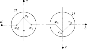
Figure 6: A graph that has an induced $\cramped{C_{4}}$ subgraph on vertices $a,c,b,d$ must have a center-center path. In this figure, the star $u$ is where $\cramped{P_{a,c}}$ and $\cramped{P_{b,c}}$ branch apart, and the star-node $v$ is where $\cramped{P_{a,c}}$ and $\cramped{P_{a,d}}$ branch apart. If $u$ and $v$ do not form a center-center path, $b$ and $d$ cannot be adjacent in the accessibility graph $G$.

Remark 2.7.

Importantly, a center-center path is defined as being an alternated path between the centers of two star-nodes, as reflected in Figure 6. In this manner, the definition excludes the possibility that, somewhere on the path between the $\cramped{c_{u}}$ and $\cramped{c_{v}}$ marker vertices, there is a star (or for that matter a prime node) which breaks the alternating path—in the sense that it requires taking at least two interior edges.

But while the definition excludes it, it is a very real possibility to keep in mind when decomposing the grammar of the tree. As we will see in Section 4 on ptolemaic graphs, specifically for the case of the clique-node $\cls{K}$, we may need to engineer the grammar in such a way that it keeps track of whether a path between two nodes is alternated (or not).

Definition 2.8.

Let $G$ be a totally decomposable graph with the reduced clique-star split-decomposition tree $T$. A clique-center path in $T$ is an alternated path $P$, such that the endpoints of $P$ are the center of a star-node $u\in V(T)$ and a marker vertex of a clique-node $v\in V(T)$ and $P$ does not contain any interior edge of the clique-node or the star-node.

Lemma 2.9 (split-decomposition tree characterization of diamond-free graphs).

Let $G$ be totally decomposable graph with the reduced clique-star split-decomposition tree $T$. $G$ does not have any induced diamonds if and only if $T$ does not have any induced clique-center paths.

Proof 2.10.

[$\Rightarrow$]  Let $T$ be a clique-star tree containing a clique-center path $P$ between the center of a star-node $u\in V(T)$ and a marker vertex of a clique-node $v\in V(T)$. We will show that the accessibility graph $G(T)$ has an induced diamond.

Let $\cramped{c_{u}}\in\cramped{G_{u}}$ and $\cramped{c_{v}}\in\cramped{G_{v}}$ be the endpoints of $P$. By an argument similar to the one in the proof of Lemma 2.5, it follows from Lemma 2.2 that there must be at least two disjoint maximal alternated paths out of $u$, each beginning at an extremity of $\cramped{G_{u}}$ and ending at leaves $a,b\in V(T)$. Similarly, there must be at least two disjoint maximal alternated paths out of the clique-node $v$ ending at leaves $c,d\in V(T)$ (Figure 7).

We can now show that this clique-center path translates to an induced diamond in the accessibility graph $G$ of $T$. Given this established labeling of the leaves $a,b,c,d$ and internal nodes $u,v$, the exact same argument outlined in the proof of Lemma 2.5 directly applies here, showing that $(a,c),(a,d),(b,c),(b,d)\in E(G)$. Similarly, it can be shown that $(a,b)\not\in E(G)$.

Where this proof diverges from the proof of Lemma 2.5 is in the existence of the edge $(c,d)\in E(G)$. This is easy to show: Let $\cramped{x_{c}},\cramped{x_{d}}\in V(\cramped{G_{v}})$ be the marker vertices of the clique-node $v$ that mark the end points of the paths out of $v$ to the leaves $c$ and $d$ respectively. We have $(c,d)\in E(G)$ by tracing the following alternated path: $c,\cramped{x_{c}},\cramped{x_{d}},d$ (see Figure 7).

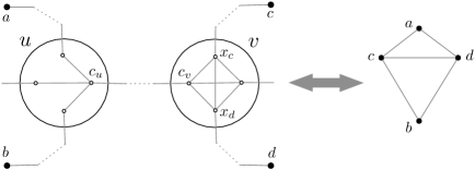
Figure 7: A clique-center path in a split-decomposition tree translates to an induced diamond in the accessibility graph.

[$\Leftarrow$]  Let $G$ be a totally decomposable graph with an induced diamond on vertices $(a,c,b,d)\in V(G)$ labeled as illustrated in Figure 7. We need to show that the reduced split-decomposition tree $T$ of $G$ has a clique-center path.

It can be shown by a similar argument to the proof of Lemma 2.5 that there must exist a star node $u\in V(T)$ that has alternated paths $\cramped{P_{a,c}}$ and $\cramped{P_{b,c}}$ out of its extremities ending in $a$ and $b$ respectively. Let $\cramped{c_{u}}\in\cramped{G_{u}}$ be the center of this star-node.

Similarly, we can show that there is a clique-node out of which maximal alternated paths lead to $c$ and $d$. Let $\cramped{P_{a,d}}$ be the unique path in $T$ between leaves $a$ and $d$, and consider the node $v\in V(T)$ where $\cramped{P_{a,c}}$ and $\cramped{P_{a,d}}$ branch apart. Let $\cramped{c_{v}}\in V(\cramped{G_{v}})$ denote the marker vertex in common between the two paths, and let $\cramped{x_{c}},\cramped{x_{d}}\in V(\cramped{G_{v}})$ be the marker vertices out of which $\cramped{P_{a,c}}$ and $\cramped{P_{a,d}}$ exit $v$ respectively. Since $(c,d)\in E(G)$, there must be an alternated path in $T$ between $c$ and $d$ that uses at most one interior edge from $\cramped{G_{v}}$, so we must have $(\cramped{x_{c}},\cramped{x_{d}})\in E(\cramped{G_{v}})$. Therefore, $\cramped{G_{v}}$ has an induced $\cramped{K_{3}}$ on the marker vertices $\cramped{x_{c}}$, $\cramped{x_{d}}$, and $\cramped{c_{v}}$. Since $T$ is a clique-star tree and $v$ cannot be a star-node, it has to be a clique node.

Finally, we need to show that $u$ and $v$ form a clique-center path. This is indeed the case since, if the path $P$ between $u$ and $v$ connected to either extremity of $\cramped{G_{u}}$, one of the following cases would occur:

• $P$ connects to the extremity of $u$ ending in $a$, which implies $(b,c),(b,d)\not\in E(G)$;

• $P$ connects to the extremity of $u$ ending in $b$, which implies $(a,c),(a,d)\not\in E(G)$;

• $P$ connects to another extremity of $u$ (if one exists), which implies $(a,c),(a,d),(b,c),(b,d)\not\in E(G)$.

Since all the above cases contradict the fact that $\set{a,b,c,d}$ induces a diamond in $G$, $P$ must be a clique-center path between $u$ and $v$.

Lemma 2.11 (Split-decomposition tree characterization of graphs without induced cliques on 4 (or more) vertices).

Let $G$ be totally decomposable graph with the reduced clique-star split-decomposition tree $T$. $G$ does not contain any induced $\cramped{K_{\geqslant 4}}$ subgraphs if and only if $T$ does not have:

• any clique-nodes of degree 4 or more;

• any alternated paths between different clique-nodes.

Proof 2.12.

[$\Rightarrow$]  We will show that for any clique-star tree $T$ breaking either of the conditions of this lemma, the accessibility graph $G(T)$ must have an induced clique on at least 4 vertices as a subgraph.

First, suppose $T$ has a clique-node of degree 4 or more. It follows from Lemma 2.3 that $G(T)$ must have an induced $\cramped{K_{\geqslant 4}}$ subgraph.

Second, suppose there are two clique-nodes $u,v\in V(T)$ connected via an alternated path $P$. Each of $\cramped{G_{u}}$ and $\cramped{G_{v}}$ must have at least three marker vertices, one of which belongs to $P$. Therefore, $u$ and $v$ each have at least two marker vertices with outgoing maximal alternated paths that end in two distinct leaves by Lemma 2.2. The four leaves at the end of these alternated paths are pairwise adjacent in $G$, thus inducing a $\cramped{K_{4}}$.

[$\Leftarrow$]  Let $G$ be a totally decomposable graph with an induced clique subgraph on 4 or more vertices, including $a,b,c,d\in V(G)$. We will show that the split-decomposition tree $T$ of $G$ breaks at least one the conditions listed in this lemma, i.e. either $T$ has a clique-node of degree 4 or more, or it has two clique-nodes (of degree 3) connected via an alternated path.

Consider the alternated paths $\cramped{P_{a,b}}$, $\cramped{P_{a,c}}$, and $\cramped{P_{a,d}}$ between the pairs of leaves $\{a,b\}$, $\{a,c\}$, and $\{a,d\}$ respectively. Let $\cramped{u_{b,c}}\in\cramped{P_{a,b}}\cap\cramped{P_{a,c}}$ be the closest internal node to $a$ in common between $\cramped{P_{a,b}}$ and $\cramped{P_{a,c}}$.

We observe that $\cramped{u_{b,c}}$ must be a clique-node. This is the case because if $\cramped{u_{b,c}}$ were a star-node, at least two of the alternated paths would have to enter $\cramped{u_{b,c}}$ at two extremities and use two interior edges of the graph label $\cramped{g_{u_{b,c}}}$. In this case, the leaves at the end of those two paths could not be adjacent in $G$.

By a symmetric argument, it can be shown that $\cramped{u_{b,d}}$, the closest internal node to $a$ in common between $\cramped{P_{a,b}}$ and $\cramped{P_{a,c}}$, must also be a clique-node.

Depending on whether or not $\cramped{u_{b,c}}$ and $\cramped{u_{b,d}}$ are distinct nodes, one of the conditions of the lemma is contradicted:

• if $\cramped{u_{b,c}}$ and $\cramped{u_{b,d}}$ are the same clique node, there are four disjoint outgoing alternated paths out it, implying that it must have a degree of at least four, contradiction the first condition of the lemma;

• if $\cramped{u_{b,c}}$ and $\cramped{u_{b,d}}$ are distinct clique nodes, they are connected by an alternated path that is a part of $\cramped{P_{a,b}}$ between them, contradicting the second condition of the lemma.

Lemma 2.13 (Split-decomposition tree characterization of graphs without pendant edges).

Let $G$ be totally decomposable graph with the reduced clique-star split-decomposition tree $T$. $G$ does not have any pendant edges if and only if $T$ does not have any star-node with its center and an extremity adjacent to leaves.

Proof 2.14.

[$\Rightarrow$]  Let $T$ be a clique-star tree, and let $u\in V(T)$ be a star-node, such that its center $\cramped{c_{u}}$ is adjacent to a leaf $a\in V(T)$ and one of its extremities $\cramped{x_{b}}$ is adjacent to a leaf $b\in V(T)$. We will show that $b$ does not have any neighbors beside $a$ in the accessibility graph $G(T)$ and thus, the edge $(a,b)$ is a pendant edge of $G(T)$.

Suppose, on the contrary, that $b$ has a neighbor $c\in V(G(T))$, $c\neq a$. Then there must be an alternated path $P$ in $T$ that connects $b$ and $c$. Note that $P$ must go through $u$, entering it at an extremity $\cramped{x_{c}}\in V(\cramped{G_{u}})$. The path $P$ must thus use two interior edges $(\cramped{x_{b}},\cramped{c_{u}})$ and $(\cramped{c_{u}},\cramped{x_{c}})$ and cannot be alternated (Figure 8).

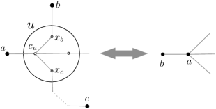
Figure 8: In a clique-star tree, a star-node with both its center and one of its extremities adjacent to leaves translates to a pendant edge in the accessibility graph.

[$\Leftarrow$]  Let $G$ be a totally decomposable graph with a pendant edge $(a,b)\in E(G)$ such that $b$ has degree 1 (Figure 8). We will show that the corresponding leaves $a$ and $b$ in the reduced clique-star tree $T$ of $G$ are attached to a star-node $u$, with its center adjacent to $a$ and one of its extremities adjacent to $b$. Let $u\in V(T)$ be the internal node to which $b$ is attached, and let $\cramped{x_{b}}\in V(\cramped{G_{u}})$ be the marker vertex adjacent to $b$.

First, we will show that $u$ is indeed a star-node and $\cramped{x_{b}}$ is one of its extremities. To do so, it suffices to show that $\cramped{x_{b}}$ has degree 1 in $\cramped{G_{u}}$. Suppose, on the contrary, that there are two marker vertices $y,z\in V(\cramped{G_{u}})$ that are adjacent to $\cramped{x_{b}}$, and consider two maximal alternated paths out of $y$ and $z$. By Lemma 2.2, these paths end at two distinct leaves of $T$, both of which much be adjacent to $b$ in $G$, contradicting the assumption that $b$ has degree 1.

Next, we will show that $a$ must be attached to the center $\cramped{c_{u}}$ of $\cramped{G_{u}}$. Otherwise, one of the following cases will occur:

• $\cramped{c_{u}}$ is adjacent to a leaf $c\in V(T)$.  In this case, we have the alternated path $b,\cramped{x_{b}},\cramped{c_{u}},c$, implying $(b,c)\in E(G)$, contradicting the assumption that $b$ has degree 1.

• $\cramped{c_{u}}$ is adjacent to a clique-node $v\in V(T)$.  With an argument similar to the previous case, it can be shown that in this case, there must exist at least two alternated paths out of $v$ that lead to leaves, all of which must be adjacent to $b$.

• $\cramped{c_{u}}$ is adjacent to the center of a star-node $v\in V(T)$.  Similar to the previous case, there must exist at least two alternated paths out extremities of $v$ that lead to leaves, all of which must be adjacent to $b$.

• $\cramped{c_{u}}$ is adjacent to an extremity of a star-node $v\in V(T)$.  This case never happens, since $T$ is assumed to be a reduced clique-star tree.

Therefore, $a$ must be attached to the center of $\cramped{G_{u}}$, so $u$ is a star-node with $a$ adjacent to its center and $b$ adjacent to one of its extremities.

Lemma 2.15 (Split-decomposition tree characterization of graphs without bridges).

Let $G$ be totally decomposable graph with the reduced clique-star split-decomposition tree $T$. $G$ does not have any bridges if and only if $T$ does not have:

• any star-node with its center and an extremity adjacent to leaves;

• any two star-nodes adjacent via their extremities, with their centers adjacent to leaves.

Proof 2.16.

We distinguish between two kinds of bridges: pendant edges and other bridges, which we will call internal bridges. Lemma 2.13 states that a star-node with its center and an extremity adjacent to leaves in $T$ corresponds to a pendant edge in $G$. Therefore, it suffices to show $G$ has no internal bridges if and only if the second condition holds in $T$.

[$\Rightarrow$]  Let $T$ be a clique-star tree, and let $u,v\in V(T)$ be two star-nodes, with the center $\cramped{c_{u}}\in\cramped{G_{u}}$ adjacent to a leaf $a\in V(T)$, the center $\cramped{c_{v}}\in\cramped{G_{v}}$ adjacent to a leaf $b\in V(T)$, and two of their extremities $\cramped{x_{u}}\in\cramped{G_{u}}$ and $\cramped{x_{v}}\in\cramped{G_{v}}$ adjacent to each other. We will show that $(a,b)$ is an internal bridge in $G(T)$.

First, let us define the following partition of the leaves of $T$ into two sets: Since every edge in a tree is a bridge, removing $(u,v)$ from $T$ breaks $T$ into two connected components. Let $\cramped{V_{u}},\cramped{V_{v}}\in V(T)$ be the leaves of these components respectively, and note that $a\in\cramped{V_{u}}$ and $b\in\cramped{V_{v}}$ (Figure 9).

Next, note that $(a,b)\in E(G(T))$ by tracing the alternated path $a,\cramped{c_{u}},\cramped{x_{u}},\cramped{x_{v}},\cramped{c_{v}},b$. To show that $(a,b)$ must be an internal bridge, it suffices We will show that the edge $(a,b)$ is a bridge in $G(T)$ by showing it does not belong to any cycles. We will then confirm that $(a,b)$ must be an internal bridge.

Suppose, on the contrary, that there $G(T)$ has a cycle $C$ of vertices $(\cramped{x_{1}}=a,\cramped{x_{2}},\dots,\cramped{x_{k-1}},\cramped{x_{k}}=b)\in\cramped{V(G(T))^{k}}$ for some $k\geqslant 3$. Clearly, $\cramped{x_{1}}=a\in\cramped{V_{u}}$. Additionally, for every edge $(\cramped{x_{i}},\cramped{x_{i+1}})\in E(G(T))$, $i=1\dots k-1$, there must be an alternated path $\cramped{P_{i}}$ in $T$ between leaves $\cramped{x_{i}}$ and $\cramped{x_{i+1}}$. Furthermore, if $\cramped{x_{i}}\in\cramped{V_{u}}$, we must also have $\cramped{x_{i+1}}\in\cramped{V_{u}}$, since otherwise, $\cramped{P_{i}}$ must use the only edge crossing the cut $\cramped{V_{u}},\cramped{V_{v}}$; this requires $\cramped{P_{i}}$ to enter and exit $u$ via two extremities of $\cramped{G_{u}}$, which requires using two interior edges from $\cramped{G_{u}}$. Applying a similar argument for every edge $(\cramped{x_{i}},\cramped{x_{i+1}})$ of $C$ up to $b$ implies that $b\in\cramped{V_{u}}$. Therefore, we must have $b\in\cramped{V_{u}}\cap\cramped{V_{v}}$, contradicting the fact that $\cramped{V_{u}}$ and $\cramped{V_{v}}$ are disjoint.

Finally, we can show via Lemma 2.2 that $(a,b)$ must be an internal bridge, by showing that $a$ and $b$ must have neighbors besides each other in $G(T))$. We will confirm this for $a$, and the argument applies symmetrically to $b$. Since $T$ is reduced, $u$ has degree at least three, so there is at least one alternating path out of an extremity of $\cramped{G_{u}}$ other than $\cramped{x_{u}}$ ending in a leaf of $T$ other than $b$, implying that $a$ must be adjacent to that leaf in $G(T)$. Similarly, $b$ must have a neighbor in $G(T)$ other than $a$. Therefore, $(a,b)$ cannot be a pendant edge and must be an internal bridge.

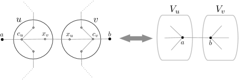
Figure 9: In a clique-star tree, a structure consisting of two star-nodes adjacent via their extremities, with their centers adjacent to leaves, translates to an internal bridge in the accessibility graph.

[$\Leftarrow$]  Let $G$ be a totally decomposable graph with an internal bridge $(a,b)\in E(G)$ (Figure 9). We show that the corresponding leaves $a$ and $b$ in the reduced clique-star tree $T$ of $G$ are respectively attached to centers of two star-node $u$ and $v$ adjacent via their extremities.

Let $u\in V(T)$ be the internal node to which $a$ is attached, and let $\cramped{c_{u}}\in V(\cramped{G_{u}})$ be the marker vertex adjacent to $a$. Similarly, let $v\in V(T)$ be the internal node to which $b$ is attached, and let $\cramped{c_{v}}\in V(\cramped{G_{v}})$ be the marker vertex adjacent to $b$.

Now, we show that $u$ and $v$ are star-nodes. Suppose, on the contrary, that $u$ is a clique-node, and note that $\cramped{G_{u}}$ must have at least two other marker vertices besides $\cramped{c_{u}}$. Consider the two maximal alternated paths $\cramped{P_{x}}$ and $\cramped{P_{y}}$ out of these two marker vertices, respectively ending in leaves $x,y\in V(T)$ by Lemma 2.2. We first observe that $(a,x)\in E(G)$ by the union of the alternated path $\cramped{P_{x}}$ and the interior edge of $\cramped{G_{u}}$ between $\cramped{c_{u}}$ and the marker vertex at the end of $\cramped{P_{x}}$. Similarly, we have $(a,y)\in E(G)$. Furthermore, $(x,y)\in E(G)$ by the union of the two alternated paths $\cramped{P_{x}}$ and $\cramped{P_{y}}$ and the interior edge of $\cramped{G_{u}}$ between the ends of these paths.The trio of vertices $a,x,y\in V(G)$ thus induces a $\cramped{C_{3}}$ in $G$, contradicting the assumption that $(a,b)$ is a bridge.

Next, we will show that $u$ and $v$ are adjacent to each other via their extremities $\cramped{x_{u}}$ and $\cramped{x_{v}}$. Otherwise, since no star centers are adjacent to extremities of other star-nodes in a reduced split-decomposition tree, $u$ and $v$ would have to be adjacent via their centers. This would constitute a center-center path, which would, by Lemma 2.5, imply that $(a,b)$ belongs to a $\cramped{C_{4}}$ and cannot be a bridge.

Finally, we confirm that $\cramped{c_{u}}$ and $\cramped{c_{v}}$, the marker vertices to which $a$ and $b$ are attached, are the centers of $\cramped{G_{u}}$ and $\cramped{G_{v}}$ respectively. It suffices to show this claim for $a$, as the argument symmetrically applies to $b$ as well. If, on the contrary, $a$ were attached to an extremity of $\cramped{G_{u}}$, the only path in $T$ between $a$ and $b$ would have to use two interior edges of $\cramped{G_{u}}$, one from $\cramped{c_{u}}$ to the center of $\cramped{G_{u}}$ and one from the center to $\cramped{x_{u}}$. This would imply $(a,b)\not\in E(G)$, a contradiction.

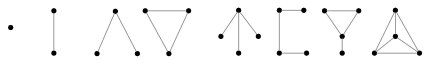
Figure 10: All block graphs on four vertices or less.

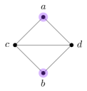
(a) A diamond.

(b) A $\cramped{C_{4}}$.

Figure 11: The class of weakly geodetic graphs can be characterized in terms of forbidden subgraphs as ($\cramped{C_{4}}$, diamond)-free. This is the case because, while in a weakly geodetic graph, a pair of vertices of distance 2 has a unique common neighbor, in an induced $\cramped{C_{4}}$ or diamond subgraph, the highlighted vertices $a$ and $b$ are of distance 2 while having at least two common neighbors $c$ and $d$.

3 Block graphs

In this section, we analyze a class of graphs called block graphs. After providing a general definition of this class, we present its well-known forbidden induced subgraph characterization, and using a lemma we proved in Section 2, we deduce a characterization of the split-decomposition tree of graphs in this class.

Block graphs are the (weakly geodetic) subset of ptolemaic graphs—themselves the (chordal) subset of distance-hereditary graphs. Thus, their split-decomposition tree is a more constrained version of that of ptolemaic graphs. As such, we use block graphs as a case study to prepare for ptolemaic graphs, for which the grammar is a bit more complicated.

3.1 Characterization.

For any graph $G$, a vertex $v$ is a cut vertex if the number of connected components is increased after removing $v$, and a block is a maximal connected subgraph without any cut vertex.

A graph is then called a block graph [Harary63] if and only if its blocks are complete graphs (or cliques) and the intersection of two blocks is either empty or a cut vertex. Block graphs are the intersection of ptolemaic graphs and weakly geodetic graphs, as was shown by Kay and Chartrand [KaCh65].

Definition 3.1 (Kay and Chartrand [KaCh65, §2]).

A graph is weakly geodetic if for every pair of vertices of distance 2 there is a unique common neighbour of them.

It is relatively intuitive to figure out from this definition, that weakly geodetic graphs are exactly ($\cramped{C_{4}}$, diamond)-free graphs, but surprisingly we were only able to find this result mentioned relatively recently [EsHoSpSr11].

Lemma 3.2.

A graph is weakly geodetic if and only if it contains no induced $\cramped{C_{4}}$ or diamond subgraphs.

Proof 3.3.

[$\Rightarrow$]  We show a weakly geodetic graph is ($\cramped{C_{4}}$, diamond)-free by arguing that graphs with induced $\cramped{C_{4}}$ subgraphs and diamonds as induced subgraphs are not weakly geodetic. This is illustrated in Figure 11, in which the highlighted pairs of vertices in a $\cramped{C_{4}}$ and a diamond are of distance 2 and have more than one neighbor in common.

[$\Leftarrow$]  Let $G$ be a ($\cramped{C_{4}}$, diamond)-free, and let $a,b\in V(G)$ be vertices of distance 2 with two neighbors $c,d\in V(G)$ in common. Since $a,b$ have distance 2, $(a,b)\not\in E(G)$. Depending on whether or not $(c,d)$ belongs to the edge set of $G$, we have $\{a,b,c,d\}$ inducing a diamond (Figure 11) or a $\cramped{C_{4}}$ (Figure 11) respectively.

Since we have established that block graphs are the subset of totally decomposable (distance-hereditary) graphs which are also ($\cramped{C_{4}}$, diamond)-free, we can now characterize their split-decomposition tree by applying our two lemmas from Section 2 and deducing the overall constraint on the split-decomposition trees that these imply.

Theorem 3.4 (split-decomposition tree characterization of block graphs).

A graph $G$ with the reduced split-decomposition tree $(T,\mathcal{F})$ is a block graph if and only if

1. $T$ is a clique-star tree;

2. the centers of all star-nodes are attached to leaves.

Proof 3.5.

We have introduced block graphs as being the intersection class of ptolemaic graphs and weakly geodetic graphs. As we will see again in Section 4, Howorka [Howorka81, §2] has shown that ptolemaic graphs are the intersection class of distance-hereditary graphs and chordal (triangulated) graphs.

A chordal graph is a graph in which any cycle of size larger than 3 has a chord; because distance-hereditary graphs are themselves $\cramped{C_{\geqslant 5}}$-free, chordal distance-hereditary (ptolemaic) graphs are the $\cramped{C_{4}}$-free distance-hereditary graphs. The additional constraint that comes with being weakly geodetic, implies that block graphs are the ($\cramped{C_{4}}$, diamond)-free distance-hereditary graphs.

The first condition in this theorem is due to the total decomposability of block graphs as a subset of distance-hereditary graphs. The second condition forbids having any center-center or clique-center paths, which, by Lemma 2.5 and Lemma 2.9 respectively, ensures that $G$ does not have any induced $\cramped{C_{4}}$ or diamond.

3.2 Rooted grammar.

Using the split-decomposition tree characterization derived above, we can provide a symbolic grammar that can be used to enumerate labeled and unlabeled block graphs.

Theorem 3.6.

The class $\cls[\bullet]{BG}$ of block graphs rooted at a vertex is specified by

$$\cls[\bullet]{BG} =\clsAtom_{\bullet}\times(\cls[C]{S}+\cls[X]{S}+\cls{K})$$ (2)

$$\cls{K} =\Set[\geqslant 2]{\clsAtom+\cls[X]{S}}$$ (3)

$$\cls[C]{S} =\Set[\geqslant 2]{\clsAtom+\cls{K}+\cls[X]{S}}$$ (4)

$$\cls[X]{S} =\clsAtom\times\Set[\geqslant 1]{\clsAtom+\cls{K}+\cls[X]{S}}\text{.}$$ (5)

This grammar is similar to that of distance-hereditary graphs [ChFuLu14]. The constraint that the centers of all star-nodes are attached to leaves means essential that the rule $\cramped{\cls[C]{S}}$ can only be reached as a starting point when we are describing what the root vertex might be connected to (from the initial rule, $\cls[\bullet]{BG}$).

For the sake of comprehensiveness, we give this proof in full detail. However since the following proofs are fairly similar, we will tend to abbreviate them.

Proof 3.7.

We begin with the rule for a star-node entered by its center,

$$\cls[C]{S}=\Set[\geqslant 2]{\clsAtom+\cls{K}+\cls[X]{S}}\text{.}$$

This equation specifies that a subtree rooted at a star-node, linked to its parent by its center, has at least 2 unordered children attached to the extremities of the star-node: each extremity can either lead to a leaf, a regular clique-node, or another star-node entered through an extremity (but not another star-node entered through its center since the tree is reduced). The lower bound of 2 children is due to the fact that in a reduced split-decomposition tree, every internal node has degree at least 3, one of which is the star-node’s center.

Next,

$$\cls[X]{S}=\clsAtom\times\Set[\geqslant 1]{\clsAtom+\cls{K}+\cls[X]{S}}\text{,}$$

corresponding to a subtree rooted at a star-node, linked to its parent by an extremity. This star-node can be be exited either via its center and lead to a leaf $\clsAtom$ (the only type of element the center of a star-node can be connected to, following Theorem 3.4), or via some extremity and lead to a leaf, a regular clique-node, or another star-node entered through an extremity (but not another star-node entered through its center, as that is forbidden in reduced trees).

Next, the equation corresponding to a clique-node,

$$\cls{K}=\Set[\geqslant 2]{\clsAtom+\cls[X]{S}}\text{.}$$

A clique-node has a degree of at least three, so a clique-rooted subtree can be exited from a set of at least two children and reach a leaf or a star-node through its extremity. It cannot reach another clique-node since the tree is reduced, and it cannot enter a star-node through its center since, again according to Theorem 3.4, star centers are only adjacent to leaves.

Finally, this equation

$$\cls[\bullet]{BG}=\clsAtom_{\bullet}\times(\cls[C]{S}+\cls[X]{S}+\cls{K})\text{,}$$

combines the previously introduced terms into a specification for rooted split-decomposition trees of block graphs, which are combinatorially equivalent to the class of rooted block graphs. It states that a rooted split-decomposition tree of a block graph consists of a distinguished leaf $\cramped{\clsAtom_{\bullet}}$, which is attached to an internal node. The internal node could be a clique-node, or a star-node entered through either its center or an extremity.

With this symbolic specification, and a computer algebra system, we may extract an arbitrary long enumeration (we’ve easily extracted 10 000 terms).

3.3 Unrooted grammar.

Applying the dissymmetry theorem to the internal nodes and edges of split-decomposition trees for block graphs gives the following grammar.

Theorem 3.8.

The class $\cls{BG}$ of unrooted block graphs is specified by

$$\cls{BG} =\cls[K]{T}+\cls[S]{T}+\cls[S-S]{T}-\cls[S\rightarrow S]{T}-\cls[S-K]{T}$$ (6)

$$\cls[K]{T} =\Set[\geqslant 3]{\clsAtom+\cls[X]{S}}$$ (7)

$$\cls[S]{T} =\clsAtom\times\cls[C]{S}$$ (8)

$$\cls[S-S]{T} =\Set[2]{\cls[X]{S}}$$ (9)

$$\cls[S\rightarrow S]{T} =\cls[X]{S}\times\cls[X]{S}$$ (10)

$$\cls[S-K]{T} =\cls{K}\times\cls[X]{S}$$ (11)

$$\cls[C]{S} =\Set[\geqslant 2]{\clsAtom+\cls{K}+\cls[X]{S}}$$ (12)

$$\cls[X]{S} =\clsAtom\times\Set[\geqslant 1]{\clsAtom+\cls{K}+\cls[X]{S}}$$ (13)

$$\cls{K} =\Set[\geqslant 2]{\clsAtom+\cls[X]{S}}$$ (14)

As noted in Subsection 1.6, in the unrooted specification, the classes denoted by $\cramped{\cls[\ldots]{T}}$ correspond to trees introduced by the dissymmetry theorem, whereas the specification of all other classes is identical to the rooted grammar for block graph split-decomposition trees given in Theorem 3.6.

Proof 3.9.

From the dissymmetry theorem, we have the following bijection linking rooted and unrooted split-decomposition trees of block graphs,

$$\cls{BG} ={{\cls{BG}}_{\circ}}+{{\cls{BG}}_{\circ-\circ}}-{{\cls{BG}}_{\circ\rightarrow\circ}}\text{.}$$

Lemma 1.8 allows us to consider only internal nodes for the rooted terms. Since block graphs are totally-decomposable into star-nodes and clique-nodes, we have the following symbolic equation for split-decomposition trees of block graphs rooted at an internal node,

$${\cls{BG}}_{\circ} =\cls[K]{T}+\cls[S]{T}\text{.}$$

Additionally, when rooting split-decomposition trees of block graphs at an undirected edge between internal nodes, the edge could either connect two star-nodes or a star-node and a clique-node (recall that clique-nodes cannot be adjacent in reduced trees by Theorem 1.6), which yields the following symbolic equation for block graph split-decomposition trees rooted at an internal undirected edge,

$${{\cls{BG}}_{\circ-\circ}} =\cls[S-S]{T}+\cls[S-K]{T}\text{.}$$

Finally, when rooting split-decomposition trees of block graphs at a directed edge between internal nodes, the edge could either go from a star-node to a clique-node, a clique-node to a star-node, or a star-node to another star-node (again, there are no adjacent clique-nodes by Theorem 1.6 of reduced trees), giving the following symbolic equation for block graph split-decomposition trees rooted at an internal directed edge,

$${{\cls{BG}}_{\circ\rightarrow\circ}} =\cls[S\rightarrow K]{T}+\cls[K\rightarrow S]{T}+\cls[S\rightarrow S]{T}\text{.}$$

Combining the above equations with the dissymmetry equation for block graph split-decomposition trees gives

$$\cls{BG} =\cls[K]{T}+\cls[S]{T}$$

$$+\cls[S-S]{T}+\cls[S-K]{T}$$

$$-\cls[S\rightarrow K]{T}-\cls[K\rightarrow S]{T}-\cls[S\rightarrow S]{T}\text{.}$$

We next observe the following bijection between ptolemaic trees rooted at an edge between a clique-node and a star-node, $\cls[S\rightarrow K]{T}\simeq\cls[K\rightarrow S]{T}$ $\simeq\cls[S-K]{T}$. This due to the fact that star- and clique-nodes are distinguishable, so an edge connecting a star-node and a clique-node bears an implicit direction. (One can, for example, define the direction to always be out of the clique-node into the star-node.) Simplifying accordingly, we arrive at Equation (6),

$$\cls{PG} =\cls[K]{T}+\cls[S]{T}+\cls[S-S]{T}-\cls[S\rightarrow S]{T}-\cls[S-K]{T}$$

We will now discuss the symbolic equations for rooted split-decomposition trees of block graphs, starting with the following equation,

$$\cls[K]{T}=\Set[\geqslant 3]{\clsAtom+\cls[X]{S}}\text{.}$$

This equation states that the split-decomposition tree of a block graph rooted at a clique-node can be specified as a set of at least three subtrees (since internal nodes in reduced split-decomposition trees have degree $\geqslant 3$), each of which can lead to either a leaf or a star-node entered through its center; they cannot lead to clique-nodes as there are no adjacent clique-nodes in reduced split-decomposition trees, and they cannot lead to star-nodes through their centers, as centers of star-nodes in block graph split-decomposition trees only connect to leaves.

Next, we will consider the equation,

$$\cls[S]{T}=\clsAtom\times\cls[C]{S}\text{.}$$

which specifies a block graph split-decomposition tree rooted at a star-node. The specification of the subtrees of the distinguished star-node depends on whether they are connected to the center or an extremity of the root. The center of the root can only be attached to a leaf, while the subtrees connected to the extremities of the distinguished star-node are exactly those specified by an $\cls[C]{S}$.

The other three rooted tree equations follow from with the same logic.

4 Ptolemaic graphs

Figure 12: Small (unrooted, unlabeled) ptolemaic graphs.

Ptolemaic graphs were introduced by Kay and Chartrand [KaCh65] as the class of graph that satisfied the same properties as a ptolemaic space. Later, it was shown by Howorka [Howorka81] that these graphs are exactly the intersection of distance-hereditary graphs and chordal graphs; beyond that, relatively little is known about ptolemaic graphs [UeUn09], and in particular, their enumeration was hitherto unknown.

4.1 Characterization.

Definition 4.1.

A graph $G$ is ptolemaic if any four vertices $u,v,w,x$ in the same connected component satisfy the ptolemaic inequality [KaCh65]:

$$d_{G}(u,v)\cdot d_{G}(w,x) \leqslant d_{G}(u,w)\cdot d_{G}(v,x)$$

$${}\quad+d_{G}(u,x)\cdot d_{G}(v,w).$$

Equivalently, ptolemaic graphs are graphs that are both chordal and distance-hereditary [Howorka81, §2].

This second characterization is the one that we will use: indeed, by a reasoning similar to that provided in the proof of Theorem 3.4, we have that distance-hereditary graphs do not contain any $\cramped{C_{\geqslant 5}}$, and chordal graphs do not contain any $\cramped{C_{\geqslant 4}}$; by virtue of being a distance-hereditary graph (described by a clique-star tree), we thus need only worry about the forbidden $\cramped{C_{4}}$ induced subgraphs. As it so happens, we already have a characterization of a split-decomposition tree which avoids such cycles.

Theorem 4.2 (split-decomposition tree characterization of ptolemaic graphs).

A graph $G$ with the reduced split-decomposition tree $(T,\mathcal{F})$ is ptolemaic if and only if

1. $T$ is a clique-star tree;

2. there are no center-center paths in $T$.

Proof 4.3.

Ptolemaic graphs are exactly the intersection of distance-hereditary graphs and chordal graphs. The first condition in this theorem addresses the fact that distance-hereditary graphs are exactly the class of totally decomposable with respect to the split-decomposition, and the second condition reflects the fact that, by Lemma 2.5, center-center paths correspond to induced $\cramped{C_{4}}$ subgraphs, the defining forbidden subgraphs for chordal graphs.

4.2 Rooted grammar.

Equipped with the characterization of a bijective split-decomposition tree representation of ptolemaic graphs, we are now ready to enumerate ptolemaic graphs. In this subsection, we begin by providing a grammar for rooted split-decomposition trees of ptolemaic graphs, which can be used to enumerate labeled ptolemaic graphs. Next, we derive the unlabeled enumeration.

Theorem 4.4.

The class $\cls[\bullet]{PG}$ of ptolemaic graphs rooted at a vertex is specified by

$$\cls[\bullet]{PG} =\clsAtom_{\bullet}\times(\cls[C]{S}+\cls[X]{S}+\cls{K})$$ (15)

$$\cls[C]{S} =\Set[\geqslant 2]{\clsAtom+\cls{K}+\cls[X]{S}}$$ (16)

$$\cls[X]{S} =(\clsAtom+\cls{\bar{K}})\times\Set[\geqslant 1]{\clsAtom+\cls{K}+\cls[X]{S}}$$ (17)

$$\cls{K} =\cls[C]{S}\times\Set[\geqslant 1]{\clsAtom+\cls[X]{S}}+\Set[\geqslant 2]{\clsAtom+\cls[X]{S}}$$ (18)

$$\cls{\bar{K}} =\Set[\geqslant 2]{\clsAtom+\cls[X]{S}}$$ (19)

Proof 4.5.

The interesting part of this grammar is that, to impose the restriction on center-center paths (condition (b) of Theorem  4.2), we must distinguish between two classes of clique-nodes, depending on the path through which we have reached them in the rooted tree:

• $\cls{\bar{K}}$: these are clique-nodes for which the most recent star-node on their ancestorial path has been exited through its center; we call these clique-nodes prohibitive to indicate that they cannot be connected to the center of a star-node;

• $\cls{K}$: all other clique-nodes, which we by contrast call regular.

Recall that the split-decomposition tree of ptolemaic graphs must, overall, satisfy the following constraints:

1. center-center paths are forbidden (Theorem 4.2);

2. internal nodes must have degree at least 3 (Thm. 1.6);

3. the center of a star-node cannot be incident to the extremity of another star-node (Theorem 1.6);

4. two clique-nodes cannot be adjacent (Theorem 1.6).

We can now prove the correctness of the grammar. We begin with the following equation

$$\cls[C]{S}=\Set[\geqslant 2]{\clsAtom+\cls{K}+\cls[X]{S}}$$

which specifies that a subtree rooted at a star-node, linked to its parent by its center, has at least 2 unordered children as the extremities of the star-node: each extremity can either lead to a leaf, a regular clique-node, or another star-node entered through an extremity. The children subtrees cannot be star-nodes entered through their center, since the tree is reduced. The lower bound of two children is due to the first condition of reduced split-decomposition trees (Theorem 1.6), which specifies that every internal node has degree at least 3.

We now consider the next equation

$$\cls[X]{S}=(\clsAtom+\cls{\bar{K}})\times\Set[\geqslant 1]{\clsAtom+\cls{K}+\cls[X]{S}}$$

The disjoint union in this equation indicates that a subtree rooted at a star-node, linked to its parent by an extremity, can be exited in two ways, either through the center, or through another extremity.

If the star-node is exited through its center, it can either enter a leaf or a prohibitive clique-node. It cannot enter a $\cls[X]{S}$ by the third condition of reduced split-decomposition trees (Theorem 1.6), and it cannot enter a $\cls[C]{S}$ as that would be a center-center path. Furthermore, it has to enter a prohibitive clique-node $\cls{\bar{K}}$ rather than a regular clique-node $\cls{K}$ to keep track of the fact that a star-node has been exited from its center on the current path and ensure that no another star-node will not be entered through its center.

If the star-node entered from an extremity is exited through an extremity, it has a set of at least one other extremity to choose from. Each of those extremities can lead to a either a leaf, a clique-node, or another star-node entered through its center. It cannot lead to an $\cls[C]{S}$, as that would be a center-center path.

We next discuss the equation

$$\cls{K}=\cls[C]{S}\times\Set[\geqslant 1]{\clsAtom+\cls[X]{S}}+\Set[\geqslant 2]{\clsAtom+\cls[X]{S}}$$

The disjoint union specifies that a subtree rooted at a regular clique-node can have exactly zero or one $\cls[C]{S}$ as a child. First, a regular-clique-rooted subtree is allowed to have a $\cls[C]{S}$ as a child, since regular clique-nodes are by definition not on potential center-center paths. However, a regular-clique-rooted subtree cannot have more than one $\cls[C]{S}$ child, since otherwise there would be a center-center path between the $\cls[C]{S}$ children through the clique-node.

The first summand corresponds to the case where the regular clique-node has exactly one $\cls[C]{S}$ as a child, which can be used to exit the tree. Additionally, the clique-node can be exited via any of the other children besides $\cls[C]{S}$ and reach either a leaf or a star-node entered through an extremity. Note that the clique-node cannot be exited into another clique-node of any kind by the second condition of reduced split-decomposition trees (Theorem 1.6), which indicates that no two clique-nodes are adjacent in a reduced split-decomposition tree.

The second summand corresponds to the case where the regular clique-node has no $\cls[C]{S}$ children. In this case, the regular clique-node can be exited via any of the remaining two or more subtrees that have not been used to enter it. After exiting the clique-node, one arrives at either a leaf or a star-node entered through its extremity. As explained above, is not possible to arrive at a clique-node, since there are no adjacent clique-nodes in reduced split-decomposition trees.

We now take a look at the equation specifying subtrees rooted at prohibitive clique-nodes

$$\cls{\bar{K}}=\Set[\geqslant 2]{\clsAtom+\cls[X]{S}}$$

A subtree rooted at a prohibitive clique-node can be exited via any of its set of at least two children and either enter a leaf or enter a star-node through its extremity. Since a prohibitive clique-nodes lies on a path from the center of a star-node, it cannot enter a $\cls[C]{S}$. Additionally, it cannot enter another clique-node of any kind since reduced clique-nodes cannot be adjacent.

Finally, the following equation

$$\cls[\bullet]{PG}=\clsAtom_{\bullet}\times(\cls[X]{S}+\cls[C]{S}+\cls{K})$$

combines all pieces into a symbolic specification for rooted ptolemaic graphs. It states that a rooted ptolemaic graph consists of a distinguished leaf $\cramped{\clsAtom_{\bullet}}$, which is attached to an internal node. The internal node could be star-node entered through either its center or an extremity, or it could be a regular clique-node.

Given this grammar for ptolemaic graphs, we can produce the exact enumeration for rooted labeled ptolemaic graphs using a computer algebraic system. Furthermore, we can derive the enumeration of unrooted labeled ptolemaic graphs by normalizing the counting sequence by the number of possible ways to distinguish a vertex as the root. This normalization is easy for labeled graphs, since the labels prevent the formation of symmetries. Therefore, since each vertex is equally likely to be chosen as the root, the number of unrooted labeled graphs of size $n$ is simply the number of rooted labeled graphs divided by $n$.

4.3 Unrooted grammar.

Theorem 4.6.

The class $\cls{PG}$ of unrooted ptolemaic graphs is specified by

$$\cls{PG} =\cls[K]{T}+\cls[S]{T}+\cls[S-S]{T}-\cls[S\rightarrow S]{T}-\cls[S-K]{T}$$ (20)

$$\cls[K]{T} =\cls[C]{S}\times\Set[\geqslant 2]{\clsAtom+\cls[X]{S}}+\Set[\geqslant 3]{\clsAtom+\cls[X]{S}}$$ (21)

$$\cls[S]{T} =\cls[C]{S}\times(\clsAtom+\cls{\bar{K}})$$ (22)

$$\cls[S-S]{T} =\Set[2]{\cls[X]{S}}$$ (23)

$$\cls[S\rightarrow S]{T} =\cls[X]{S}\times\cls[X]{S}$$ (24)

$$\cls[S-K]{T} =\cls{K}\times\cls[X]{S}+\cls{\bar{K}}\times\cls[C]{S}$$ (25)

$$\cls[C]{S} =\Set[\geqslant 2]{\clsAtom+\cls{K}+\cls[X]{S}}$$ (26)

$$\cls[X]{S} =(\clsAtom+\cls{\bar{K}})\times\Set[\geqslant 1]{\clsAtom+\cls{K}+\cls[X]{S}}$$ (27)

$$\cls{K} =\cls[C]{S}\times\Set[\geqslant 1]{\clsAtom+\cls[X]{S}}+\Set[\geqslant 2]{\clsAtom+\cls[X]{S}}$$ (28)

$$\cls{\bar{K}} =\Set[\geqslant 2]{\clsAtom+\cls[X]{S}}$$ (29)

Proof 4.7.

Applying the dissymmetry theorem in a similar manner to the proof of the unrooted grammar of block graphs, we obtain the following formal equation:

$$\begin{split}\cls{PG}&=\cls[K]{T}+\cls[S]{T}+\cls[S-S]{T}+\cls[S-K]{T}\\ &-\cls[S\rightarrow K]{T}-\cls[K\rightarrow S]{T}-\cls[S\rightarrow S]{T}\text{.}\end{split}$$

Notably, even though we distinguish between prohibitive $\cls{\bar{K}}$ and regular $\cls{K}$ clique-nodes in the rooted grammar, this distinction disappears when rerooting the trees for the dissymmetry theorem. This is because the prohibitive or regular nature of a clique-node depends on an implicitly directed path leading to it from the root; however when rerooting the tree, the clique-node in question becomes the new root, and all (implicitly directed) paths originate from it.

We can then simplify the dissymmetry theorem equation above in the same manner as for block graphs:

$$\cls{PG} =\cls[K]{T}+\cls[S]{T}+\cls[S-S]{T}-\cls[S\rightarrow S]{T}-\cls[S-K]{T}\text{.}$$

We then discuss the rerooted terms of the grammar, starting with the following equation,

$$\cls[K]{T} =\cls[C]{S}\times\Set[\geqslant 2]{\clsAtom+\cls[X]{S}}+\Set[\geqslant 3]{\clsAtom+\cls[X]{S}}\text{.}$$

The disjoint union translates the fact that in a ptolemaic tree rerooted at a clique-node, the root can have either zero or one $\cls[C]{S}$ as a subtree. (A clique-node having more than one $\cls[C]{S}$ subtree would induce a center-center path, which cannot exist in ptolemaic split-decomposition trees by Theorem 4.2.)

The first summand corresponds to the case where the clique-node at which the split-decomposition tree is rooted has one $\cls[C]{S}$ as a subtree. The clique-node root can have a set of at least two other subtrees, each of which can lead to either a leaf or a star-node entered from an extremity.

The second summand corresponds to the case where the clique-node at which the split-decomposition tree is rooted has no $\cls[C]{S}$ subtrees, in which case it can have a set of at least three other subtrees leading to leaves or $\cls[X]{S}$ nodes, but not clique-nodes or $\cls[C]{S}$ as explained.

Next, we will consider the equation,

$$\cls[S]{T} =\cls[C]{S}\times(\clsAtom+\cls{\bar{K}})$$

which specifies a ptolemaic split-decomposition tree rooted at a star-node. The specification of the subtrees of the distinguished star-node depends on whether they are connected to the center or an extremity of the star-node. The subtrees connected to the extremities of the distinguished star-node are exactly those specified by an $\cls[C]{S}$, and the subtree attached to the center of the distinguished star-node can lead to either a leaf or a prohibitive clique-node.

The other three rooted tree equations follow from with the same logic.

The first few terms of the enumeration of unlabeled, unrooted ptolemaic graphs (among others) are available in the Table LABEL:tab:enum-block-ptol at the end of this paper.

5 2,3-Cactus, 3-Cactus and 4-Cactus Graphs

The definition of cactus graphs is similar to that of a block graphs. Yet whereas in block graphs (discussed in Section 3), the blocks are cliques, in a cactus graph the blocks are cycles. Thus, just as block graphs can be called clique trees, cacti can be seen as “cycle trees”. An alternate definition:

Definition 5.1.

A cactus is a connected graphs in which every edge belongs to at most one cycle [HaPa73]

We can also conjure further variations on this definition, with cactus graphs having as blocks, cycles that have size constrained to a set of positive integers; thus given a set of integers $\Omega$, an $\Omega$-cactus graph is the class of cactus graphs of which the cycles have size $m\in\Omega$. In this section, we discuss cactus graphs for the sets: $\Omega=\set{2,3}$, $\Omega=\set{3}$ and $\Omega=\set{4}$, following an article by Harary and Uhlenbeck [HaUh53], who use dissimilarity characteristics derived from Otter’s theorem [Otter48].

5.1 2,3-Cactus Graphs.

In this section, we enumerate the family of cactus graphs with $\Omega=\{2,3\}$. The class of 2,3-cactus graphs is equivalent to the intersection of block graphs and of cactus graphs, not to be confused with the class of block-cactus graphs (which are the union of block graphs and cactus graphs [RaVo98]).

Theorem 5.2 (split-decomposition tree characterization of 2,3-cactus graphs).

A graph $G$ with the reduced split-decomposition tree $(T,\mathcal{F})$ is a block-cactus graph if and only if

1. $T$ is a clique-star tree;

2. every clique-node has degree 3;

3. the center of all star-nodes are attached to leaves;

Proof 5.3.

This split-decomposition tree characterization is identical to the characterization for 3-cactus graphs, except the last condition in the characterization of 3-cacti (stating that leaves cannot be attached to extremities of star-nodes) is missing here. As we outlined in the proof of the characterization of 3-cacti, a leaf attached to a an extremity of an star-node corresponds to a vertex of degree 1 in the original graph. Unlike with 3-cacti, which required that all vertices be in some cycle of size 3, having such a vertex of degree 1 here corresponds to a $\cramped{C_{2}}$ and is allowed. Therefore, the correctness of this characterization follows from the proof of the characterization for 3-cactus graphs.

Theorem 5.4.

The class $\cls[\bullet]{TTCG}$ of 2,3-cactus graphs rooted at a vertex is specified by

$$\cls[\bullet]{TTCG} =\clsAtom_{\bullet}\times(\cls[C]{S}+\cls[X]{S}+\cls{K})$$ (30)

$$\cls[C]{S} =\Set[\geqslant 2]{\clsAtom+\cls{K}+\cls[X]{S}}$$ (31)

$$\cls[X]{S} =\clsAtom\times\Set[\geqslant 1]{\clsAtom+\cls{K}+\cls[X]{S}}$$ (32)

$$\cls{K} =\Set[=2]{\clsAtom+\cls[X]{S}}$$ (33)

Theorem 5.5.

The class $\cls{TTCG}$ of unrooted 2,3-cactus graphs is specified by

$$\cls{TTCG} =\cls[K]{T}+\cls[S]{T}+\cls[S-S]{T}-\cls[S\rightarrow S]{T}-\cls[S-K]{T}$$ (34)

$$\cls[K]{T} =\Set[=3]{\clsAtom+\cls[X]{S}}$$ (35)

$$\cls[S]{T} =\clsAtom\times\cls[C]{S}$$ (36)

$$\cls[S-S]{T} =\Set[2]{\cls[X]{S}}$$ (37)

$$\cls[S\rightarrow S]{T} =\cls[X]{S}\times\cls[X]{S}$$ (38)

$$\cls[S-K]{T} =\cls{K}\times\cls[X]{S}$$ (39)

$$\cls[C]{S} =\Set[\geqslant 2]{\clsAtom+\cls{K}+\cls[X]{S}}$$ (40)

$$\cls[X]{S} =\clsAtom\times\Set[\geqslant 1]{\clsAtom+\cls{K}+\cls[X]{S}}$$ (41)

$$\cls{K} =\Set[=2]{\clsAtom+\cls[X]{S}}$$ (42)

5.2 3-Cactus Graphs

We now enumerate the family of cactus graph that is constrained to $\Omega=\{3\}$, which we refer to as the family as 3-cacti or triangular cacti.

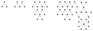
Figure 13: Small (unrooted, unlabeled) triangular cacti.

Lemma 5.6 (Forbidden subgraph characterization of 3-cacti).

A graph $G$ is a triangular cactus if and only if $G$ is a block graph with no bridges or induced $\cramped{K_{\geqslant 4}}$.

Proof 5.7.

[$\Rightarrow$]  Given a triangular cactus $G$, we will show that $G$ is a block graph and does not have any bridges or induced $\cramped{K_{\geqslant 4}}$.

We first note that $G$ is a block graphs by showing that it is ($\cramped{C_{\geqslant 4}}$, diamond)-free. There cannot be any induced $\cramped{C_{\geqslant 4}}$ in $G$, because every edge of a 3-cactus is in exactly one triangle and no other cycle. There cannot be any induced diamonds in a $G$ because diamonds have an edge in common between two cycles.

We next observe that $G$ cannot have bridges, as a bridge is by definition not part of any cycles, including triangles. Furthermore, $G$ cannot have any induced cliques on 4 or more vertices, as such a clique would involve edges shared between triangles. Therefore, $G$ must be a block graph and with no pendant edges or induced $\cramped{K_{\geqslant 4}}$.

[$\Leftarrow$]  Given a block graph $G$ without any bridges or induced $\cramped{K_{\geqslant 4}}$, we need to show that $G$ is a 3-cactus. We do so by showing that every edge $(a,b)\in E(G)$ is in exactly one triangle and no other cycle.

First, since $(a,b)$ cannot be a bridge, it must lie on some cycle $C$. Since $G$ is a block graph and thus $\cramped{C_{\geqslant 4}}$-free, $C$ must be a triangle.Furthermore, if $(a,b)$ belonged to another cycle $C^{\prime}$, by the same argument, $C^{\prime}$ would also be a triangle. Let $c$ be the third vertex of $C$ other than $a$ and $b$, and let $c^{\prime}$ the third vertex of $C^{\prime}$. Depending on the adjacency of $c$ and $c^{\prime}$, we have one of the following two cases:

• $(c,c^{\prime})\in E(G)$, in which case $\set{a,c,b,c^{\prime}}$ induces a $\cramped{K_{4}}$, which we assumed $G$ does not include;

• $(c,c^{\prime})\not\in E(G)$, in which case $\set{a,c,b,c^{\prime}}$ induces a diamond, which $G$, as a block graph, cannot contain.

Therefore, no such cycle $C^{\prime}$ can exist, implying that $(a,b)$ belongs to one and exactly one triangle in $G$ and no other cycle. Extending this argument to all edges of $G$ ensures that $G$ is a 3-cactus.

Theorem 5.8 (split-decomposition tree characterization of 3-cacti).

A graph $G$ with the reduced split-decomposition tree $(T,\mathcal{F})$ is a triangular cactus graph if and only if

1. $T$ is a clique-star tree;

2. the centers of all star-nodes are attached to leaves;

3. the extremities of star-nodes are only attached to clique-nodes;

4. every clique-node has degree 3.

Proof 5.9.

By Lemma 5.6, we know that 3-cacti can be described exactly as the class of block graphs with no bridges or induced $\cramped{K_{\geqslant}4}$.

The first and second conditions of this theorem duplicate the split-decomposition tree characterization of block graphs outlined in Theorem 3.4.

The third condition uses Lemma 2.15 to forbid bridges. Since by the second condition, all star centers in $T$ are adjacent to leaves, a star extremity adjacent to a leaf of $T$ would correspond to a bridge in the form of a pendant edge in $G$, and a star extremity adjacent to another star extremity would correspond to a non-pendant bridge in $G$.

Finally, the last condition applies Lemma 2.11 to disallow $\cramped{K_{\geqslant}4}$, the last set of forbidden induced subgraphs for 3-cactus.

The split-decomposition tree characterization of 3-cacti derived in the previous section naturally defines the following symbolic grammar for rooted block graphs.

Theorem 5.10.

The class $\cls[\bullet]{TCG}$ of triangular cactus graphs rooted at a vertex is specified by

$$\cls[\bullet]{TCG} =\clsAtom_{\bullet}\times(\cls[C]{S}+\cls{K})$$ (43)

$$\cls[C]{S} =\Set[\geqslant 2]{\cls{K}}$$ (44)

$$\cls[X]{S} =\clsAtom\times\Set[\geqslant 1]{\cls{K}}$$ (45)

$$\cls{K} =\Set[=2]{\clsAtom+\cls[X]{S}}$$ (46)

Theorem 5.11.

The class $\cls{TCG}$ of unrooted triangular cactus graphs is specified by

$$\cls{TCG} =\cls[K]{T}+\cls[S]{T}-\cls[S-K]{T}$$ (47)

$$\cls[K]{T} =\Set[=3]{\clsAtom+\cls[X]{S}}$$ (48)

$$\cls[S]{T} =\clsAtom\times\cls[C]{S}$$ (49)

$$\cls[S-K]{T} =\cls{K}\times\cls[X]{S}$$ (50)

$$\cls[C]{S} =\Set[\geqslant 2]{\cls{K}}$$ (51)

$$\cls[X]{S} =\clsAtom\times\Set[\geqslant 1]{\cls{K}}$$ (52)

$$\cls{K} =\Set[\geqslant 2]{\clsAtom+\cls[X]{S}}$$ (53)

6 Conclusion

In this paper, we follow the ideas of Gioan and Paul [GiPa12] and Chauve et al. [ChFuLu14], and provide full analyses of several important subclasses of distance-hereditary graph. Some of these analyses have lead us to uncover previously unknown enumerations (ptolemaic graphs, …), while for other classes for which enumerations were already known (block graphs, 2,3-cactus and 3-cactus graphs), we have provided symbolic grammars which are a more powerful starting point for future work: such as parameter analyses, exhaustive and random generation and the empirical analyses that the latter enables, etc.. For instance, Iriza [Iriza15, §7] provided a nice tentative preview of the type of results unlocked by these grammars, when he empirically observed the linear growth of clique-nodes and star-nodes in the split-decomposition tree of a random distance-hereditary graph.

Our main idea is encapsulated in Section 2: we think that the split-decomposition, coupled with analytic combinatorics, is a powerful way to analyze classes of graphs specified by their forbidden induced subgraph. This is remarkably noteworthy, because forbidden characterizations are relatively common, and yet they generally are very difficult to translate to specifications. What we show is that this can be (at least for subclasses of distance-hereditary graphs which are totally decomposable by the split-decomposition) fairly automatic, in keeping with the spirit of analytic combinatorics:

1. identify forbidden induced subgraphs;

2. translate each forbidden subgraph into constraints on the (clique-star) split-decomposition tree;

3. describe rooted grammar, apply unrooting, etc..

This allows us to systematically derive the grammar of a number of well-studied classes of graphs, and to compute full enumerations, asymptotic estimates, etc.. In Figure 14, for instance, we have used the results from this paper to provide some intuition as to the relative “density” of these graph classes. A fairly attainable goal would be to use the asymptotics estimates which can be derived automatically from the grammars, to compute the asymptotic probability that a random block graph is also a 2,3-cactus graph.

Naturally, this raises a number of interesting questions, but possibly the most natural one to ask is: can we expand this methodology beyond distance-hereditary graphs, to classes for which the split-decomposition tree contains prime nodes (which are neither clique-nodes nor star-nodes).

Beyond distance-hereditary graphs, another perfect (pun intended) candidate is the class of parity graphs: these are the graphs whose split-decomposition tree has prime nodes that are bipartite graphs. But while bipartite graphs have been enumerated by Hanlon [Hanlon79], and more recently Gainer-Dewar and Gessel [GaGe14], it is unclear whether this is sufficient to derive a grammar for parity graphs. Indeed, the advantage of the degenerate nodes (clique-nodes and star-nodes) is that their symmetries are fairly uncomplicated (all the vertices of a clique are undistinguished; all the vertices of a star, save the center, are undistinguished), as is in fact their enumeration (for each given size, there is only one clique or one star). An empirical study by Shi [ShLu15] showed that lower and upper bounds can be derived by plugging in the enumeration as an artificial generating function—either assuming all vertices of a bipartite prime node to be distinguished or undistinguished.

Other classes present a similar challenge, in that the subset of allowable prime nodes is itself too challenging.

A likely more fruitful direction to pursue this work is to first start with classes of graphs which have small, predictable subsets of prime nodes. We discovered one such family of classes in a paper by Harary and Uhlenbeck [HaUh53]; in this paper, they discuss the enumeration of unlabeled and unrooted 3-cactus graphs and 4-cactus graphs (which we studied and enumerated using a radically different methodology in this paper), while suggesting that they would have liked to provide some general methodology to obtain the enumeration of $m$-cactus graphs, for generalized polygons on $m$ sides.

There is some evidence to suggest that $m$-cactus graphs would yield split-decomposition trees with prime nodes that are undirected cycles of size $m$; likewise the split-decomposition tree of a general cactus graph (in which the blocks are cycles of any size larger than 3) would likely have prime nodes that are undirected cycles. In the same vein, block-cactus graphs (which are the union of the block graphs enumerated in Section 3, and of generalized cactus graphs) would likely also have the same type of prime nodes. All of these are more manageable subset, and it is likely that the various intersection classes with cactus graphs would be a more promising avenue by which to determine whether the split-decomposition can be reliably used for the enumeration of supersets of distance-hereditary graphs.

Graph Class	Number
General [Sloane, A000088]	$2.86\times\cramped{10^{685}}$
General Connected [Sloane, A001349]	$2.86\times\cramped{10^{685}}$
Distance-Hereditary [ChFuLu14]	$3.38\times\cramped{10^{56}}$
3-Leaf Power [ChFuLu14]	$8.40\times\cramped{10^{37}}$
Ptolemaic	$3.78\times\cramped{10^{50}}$
Block	$1.44\times\cramped{10^{40}}$
2,3-Cacti	$1.55\times\cramped{10^{38}}$
3-Cacti	$9.13\times\cramped{10^{16}}$
4-Cacti	$5.73\times\cramped{10^{14}}$

Table 1: Number of unlabeled graphs of size $n=73$ for different graph classes.

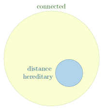
(a) Ratio of the size of distance-hereditary graphs to general connected graphs on a logarithmic scale.

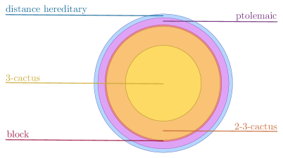
(b) Ratios of the size of various subsets of distance-hereditary graphs on a logarithmic scale.

Figure 14: Illustration of the ratios of sizes of various graph classes, for $n=73$ as depicted in Table 1. The radii are the square roots of the ratios of the logarithms of the enumeration for a given class to the logarithm of the enumeration for the base class. In addition, only strict subsets are displayed on the right. For instance, 3-leaf power graphs are a subset of ptolemaic graphs, since their characterization [GiPa12, §3.3] does not allow for center-center paths; but they are not a subset of block graphs. Similarly, we cannot represent 4-cacti as they have no intersection with 3-cacti, and it is not physically possible to represent them here given our logarithmic scale.