An Exact Enumeration of Distance-Hereditary Graphs

Abstract

Distance-hereditary graphs form an important class of graphs, from the theoretical point of view, due to the fact that they are the totally decomposable graphs for the split-decomposition. The previous best enumerative result for these graphs is from Nakano et al. (J. Comp. Sci. Tech., 2007), who have proven that the number of distance-hereditary graphs on $n$ vertices is bounded by $\cramped{2^{\lceil 3.59n\rceil}}$.

In this paper, using classical tools of enumerative combinatorics, we improve on this result by providing an exact enumeration of distance-hereditary graphs, which allows to show that the number of distance-hereditary graphs on $n$ vertices is tightly bounded by $\cramped{(7.24975\ldots)^{n}}$—opening the perspective such graphs could be encoded on $3n$ bits. We also provide the exact enumeration and asymptotics of an important subclass, the 3-leaf power graphs.

Our work illustrates the power of revisiting graph decomposition results through the framework of analytic combinatorics.

Introduction

The decomposition of graphs into tree-structures is a fundamental paradigm in graph theory, with algorithmic and theoretical applications [4]. In the present work, we are interested in the split-decomposition, introduced by Cunningham and Edmonds [8, 9] and recently revisited by Gioan et al. [19, 20, 6]. For the classical modular and split-decomposition, the decomposition tree of a graph $G$ is a tree (rooted for the modular decomposition and unrooted for the split decomposition) of which the leaves are in bijection with the vertices of $G$ and whose internal nodes are labeled by indecomposable (for the chosen decomposition) graphs; such trees are called graph-labeled trees by Gioan and Paul [19]. Moreover, there is a one-to-one correspondence between such trees and graphs. The notion of a graph being totally decomposable for a decomposition scheme translates into restrictions on the labels that can appear on the internal nodes of its decomposition tree. For example, for the split-decomposition, totally decomposable graphs are the graphs whose decomposition tree’s internal nodes are labeled only by cliques and stars; such graphs are called distance-hereditary graphs. They generalize the well-known cographs, the graphs that are totally decomposable for the modular decomposition, and whose enumeration has been well studied, in particular by Ravelomanana and Thimonier [25], also using techniques from analytic combinatorics

Efficiently encoding graph classes is naturally linked to the enumeration of such graph classes. Indeed the number of graphs of a given class on $n$ vertices implies a lower bound on the best possible encoding one can hope for. Until recently, few enumerative properties were known for distance-hereditary graphs, unlike their counterpart for the modular decomposition, the cographs. The best result so far, by Nakano et al. [23], relies on a relatively complex encoding on $4n$ bits, whose detailed analysis shows that there are at most $\cramped{2^{\lfloor 3.59n\rfloor}}$ unlabeled distance-hereditary graphs on $n$ vertices. However, using the same techniques, their result also implies an upper-bound of $2^{3n}$ for the number of unlabeled cographs on $n$ vertices, which is far from being optimal for these graphs, as it is known that, asymptotically, there are $C\cramped{d^{n}}/\cramped{n^{3/2}}$ such graphs where $C=0.4126\dots$ and $d=3.5608\dots$ [25]. This suggests there is room for improving the best upper bound on the number of distance-hereditary graphs provided by Nakano et al. [23], which was the main purpose of our present work.

This paper.

Following a now well established approach, which enumerates graph classes through a tree representation, when available (see for example the survey by Giménez and Noy [18] on tree-decompositions to count families of planar graphs), we provide combinatorial specifications, in the sense of Flajolet and Sedgewick [16], of the split-decomposition trees of distance-hereditary graphs and 3-leaf power graphs, both in the labeled and unlabeled cases. From these specifications, we can provide exact enumerations, asymptotics, and leave open the possibility of uniform random samplers allowing for further empirical studies of statistics on these graphs (see Iriza [22]).

In particular, we show that the number of distance-hereditary graphs on $n$ vertices is bounded from above by $\cramped{2^{3n}}$, which naturally opens the question of encoding such graphs on $3n$ bits, instead of $4n$ bits as done by Nakano et al. [23]. We also provide similar results for 3-leaf power graphs, an interesting class of distance hereditary graphs, showing that the number of 3-leaf power graphs on $n$ vertices is bounded from above by $\cramped{2^{2n}}$.

Main results.

Our main contribution is to introduce the idea of symbolically specifying the trees arising from the split-decomposition, so as to provide the (previously unknown) exact enumeration of certain important classes of graphs.

Our grammars for distance-hereditary graphs are in Subsection 3, and our grammars for 3-leaf power graphs are in Subsection 2. We provide here the corollary that gives the beginning of the exact enumerations for the unlabeled and unrooted versions of both classes.

Corollary 0.1 (Enumeration of connected, unlabeled, unrooted distance-hereditary graphs).

The first few terms of the enumeration, EIS A00000, are

$$1,1,2,6,18,73,308,1484,7492,40010,220676,$$

$$\qquad 1253940,7282316,43096792,259019070,$$

$$\qquad 1577653196,9720170360,60492629435\ldots$$

and the asymptotics is $c\cdot\cramped{7.249751250\ldots^{n}}\cdot\cramped{n^{-5/2}}$ with $c\approx 0.02337516194\ldots$.

Corollary 0.2 (Enumeration of connected, unlabeled, unrooted $3$-leaf power graphs).

The first few terms of the enumeration, EIS A00000, are

$$1,1,2,5,12,32,82,227,629,1840,5456,16701,$$

$$\qquad 51939,164688,529070,1722271,5664786,$$

$$\qquad 18813360,62996841,212533216\ldots$$

and the asymptotics is $c\cdot\cramped{3.848442876\ldots^{n}}\cdot\cramped{n^{-5/2}}$ with $c\approx 0.70955825396\ldots$.

1 Definitions and Preliminaries

For a graph $G$, we denote by $V(G)$ its vertex set and $E(G)$ its edge set. Moreover, for a vertex $x$ of a graph $G$, we denote by $N(x)$ the neighbourhood of $x$, that is the set of vertices $y$ such that $\{x,y\}\in E(G)$; this notion extends naturally to vertex sets: if $\cramped{V_{1}}\subseteq V(G)$, then $N(\cramped{V_{1}})$ is the set of vertices defined by the (non-disjoint) union of the neighbourhoods of the vertices in $\cramped{V_{1}}$. Finally, the subgraph of $G$ induced by a subset $\cramped{V_{1}}$ of vertices is denoted by $G[\cramped{V_{1}}]$.

A graph on $n$ vertices is labeled if its vertices are identified with the set $\{1,\dots,$ $n\}$, with no two vertices having the same label. A graph is unlabeled if its vertices are indistinguishable.

A clique on $k$ vertices, denoted $\cramped{K_{k}}$ is the complete graph on $k$ vertices (i.e., there exists an edge between every pair of vertices). A star on $k$ vertices, denoted $\cramped{S_{k}}$, is the graph with one vertex of degree $k-1$ (the center of the star) and $k-1$ vertices of degree $1$ (the extremities of the star).

1.1 Split-decomposition trees.

We first introduce the notion of graph-labeled tree, due to Gioan and Paul [19], then define the split-decomposition and the corresponding tree, described as a graph-labeled tree.

Definition 1.1.

A graph-labeled tree $(T,\mathcal{F})$ is a tree $T$ in which every internal node $v$ of degree $k$ is labeled by a graph $\cramped{G_{v}}\in\mathcal{F}$ on $k$ vertices, such that there is a bijection $\cramped{\rho_{v}}$ from the edges of $T$ incident to $v$ to the vertices of $\cramped{G_{v}}$.

Definition 1.2.

A split [8] of a graph $G$ with vertex set $V$ is a bipartition $(\cramped{V_{1}},\cramped{V_{2}})$ of $V$ (i.e., $V=\cramped{V_{1}}\cup V_{2}$, $\cramped{V_{1}}\cap\cramped{V_{2}}=\emptyset$) such that

1. $|V_{1}|>2$ and $|V_{2}|>2$;

2. every vertex of $N(V_{1})$ is adjacent to every of $N(V_{2})$.

A graph without any split is called a prime graph. A graph is degenerate if any partition of its vertices without a singleton part is a split: cliques and stars are the only such graphs.

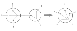
(a) Example of a star-join.

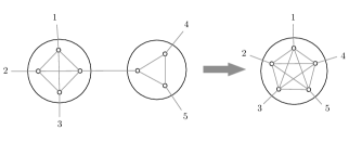
(b) Example of a clique-join.

Figure 1: The star-join and clique-join operations result in the merging of two internal nodes of a split-decomposition tree. A split-decomposition tree in which neither one of these operations may be applied (and in which all non-clique and non-star nodes are prime nodes) is said to be reduced.

Informally, the split-decomposition of a graph $G$ consists in finding a split $(\cramped{V_{1}},\cramped{V_{2}})$ in $G$, followed by decomposing $G$ into two graphs $\cramped{G_{1}}=G[\cramped{V_{1}}\cup\{\cramped{x_{1}}\}]$ where $\cramped{x_{1}}\in N(\cramped{V_{1}})$ and $\cramped{G_{2}}=G[\cramped{V_{2}}\cup\{\cramped{x_{2}}\}]$ where $\cramped{x_{1}}\in N(\cramped{V_{2}})$ and then recursively decomposing $\cramped{G_{1}}$ and $\cramped{G_{2}}$. This decomposition naturally defines an unrooted tree structure of which the internal vertices are labeled by degenerate or prime graphs and whose leaves are in bijection with the vertices of $G$, called a split-decomposition tree. A split-decomposition tree $(T,\mathcal{F})$ with $\mathcal{F}$ containing only cliques with at least three vertices and stars with at least three vertices is called a clique-star tree.

It can be shown that the split-decomposition tree of a graph might not be unique (i.e., that several decompositions sequences of a given graph can lead to different split-decomposition trees), but following Cunningham [8], we obtain the following uniqueness result, reformulated in terms of graph-labeled trees by Gioan and Paul [19].

[Cunningham [8]] For every connected graph $G$, there exists a unique split-decomposition tree such that:

1. every non-leaf node has degree at least three;

2. no tree edge links two vertices with clique labels;

3. no tree edge links the center of a star to the extremity of another star.

Such a tree is called reduced, and this theorem establishes a one-to-one correspondence between graphs and their reduced split-decomposition trees. So enumerating the split-decomposition trees of a graph class provides an enumeration for the corresponding graph class, and we rely on this property in the following sections.

1.2 Decomposable structures.

In order to enumerate classes of split-decomposition trees, we use the framework of decomposable structures, described by Flajolet and Sedgewick [16]. We refer the reader to this book for details and outline below the basics idea.

We denote by $\mathcal{Z}$ the combinatorial family composed of a single object of size $1$, usually called atom (in our case, these refer to a leaf of a split-decomposition tree, i.e., a vertex of the corresponding graph).

Given two disjoint families ${\mathcal{A}}$ and ${\mathcal{B}}$ of combinatorial objects, we denote by ${\mathcal{A}}+{\mathcal{B}}$ the disjoint union of the two families and by ${\mathcal{A}}\times{\mathcal{B}}$ the Cartesian product of the two families.

Finally, we denote by ${\text{\sc Set}}\left({\mathcal{A}}\right)$ (resp. $\cramped{{\text{\sc Set}}_{\geqslant k}\left({\mathcal{A}}\right)}$, $\cramped{{\text{\sc Set}}_{k}\left({\mathcal{A}}\right)}$) the family defined as all sets (resp. sets of size at least $k$, sets of size exactly $k$) of objects from ${{\mathcal{A}}}$, and by $\cramped{{\text{\sc Seq}}_{\geqslant k}\left({\mathcal{A}}\right)}$, the family defined as all sequences of at least $k$ objects from ${{\mathcal{A}}}$.

Remark 1.3.

Because this paper deals with classes both rooted (either at a vertex/leaf or an internal node) and unrooted, we use some notations to keep these distinct. But these notations are purely for clarity.

For instance, while we use $\cramped{\mathcal{Z}_{\bullet}}$ to denote a rooted vertex, and $\mathcal{Z}$ to denote an unrooted vertex, these are both translated in the same way in the associated generating functions and enumerations.

Remark 1.4.

Decomposable structures specified by these grammars can either be:

• labeled: in a given object, each atom is labeled by a distinct number between 1 and $n$ (the size of the object); this means that each “skeleton” of an object appears in $n!$ copies, for each of the possible way of labeling its individual atoms, and because each atom is distinguished, there are no symmetries;

• or unlabeled: in which case, an atom is indistinguishable from the next, and so certain symmetries must be taken into account (so that two objects which are not decomposed in the same way but have the same ultimate shape are not counted twice).

It is often the case that enumerations for labeled classes are easier to obtain than for unlabeled ones. Our grammars allow to derive generating functions, enumerations, and asymptotics for both.

2 3-Leaf Power Graphs

The first class that we discuss is that of $3$-leaf power graphs: a chordal subset of distance-hereditary graphs.

Definition 2.1.

A graph $G=(V,E)$ is a $k$-leaf power graph, if there is a tree $T$ (called a $k$-leaf root of graph $G$) such that:

1. the leaves of $T$ are the vertices $V$;

2. there is an edge $xy\in E$ if and only if the distance in $T$ between leaves $x$ and $y$ is at most $k$, $\cramped{d_{T}}(x,y)\leqslant k$.

These families of graphs are relevant to phylogenetics [24]: from the the pairwise genetic distance between a collection of species (which is a graph), it is desirable to establish a tree which highlights the most likely ancestry (or more broadly, the evolutionary relationships) relations between species.

We begin with the enumeration of 3-leaf power graphs, the smaller combinatorial class, because the application of the dissymmetry theorem (used to obtain an enumeration of the unrooted class given the grammar for some rooted version of the class) in Subsection 2.3 is less involved for 3-leaf power graphs than it is for distance-hereditary graphs.

2.1 Grammar from the split-decomposition.

The starting point is the characterization of the split-decomposition tree of 3-leaf power graphs, as introduced by Gioan and Paul [19].

[Characterization of $3$-leaf power split-decomposition tree [19, § 3.3]] A connected graph $G=(V,E)$ is a $3$-leaf power graph if and only if:

1. its split-decomposition tree $ST(G)$ is a clique-star tree (implies that $G$ is distance-hereditary);

2. the set of star-nodes forms a connected subtree of $T$;

3. the center of a star-node is incident either to a leaf or a clique node.

This is unsurprising given that an alternate (perhaps more pertinent) characterization is that a 3-leaf power graph can be obtained from a tree by replacing every vertex by a clique of arbitrary size.

Theorem 2.2.

The class ${{\mathcal{\text{3}LP}}_{\bullet}}$ of $3$-leaf power graphs rooted at a vertex is specified by

(2.1) $${\mathcal{\text{3}LP}}_{\bullet} ={\mathcal{L}}_{\bullet}\times\left({\mathcal{S}}_{C}+{\mathcal{S}}_{X}\right)+{\mathcal{K}}_{\bullet}$$

(2.2) $${\mathcal{S}}_{C} ={\text{\sc Set}}_{\geqslant 2}\left({\mathcal{L}}+{\mathcal{S}}_{X}\right)$$

(2.3) $${\mathcal{S}}_{X} ={{\mathcal{L}}}\times{\text{\sc Set}}_{\geqslant 1}\left({\mathcal{L}}+{\mathcal{S}}_{X}\right)$$

(2.4) $${\mathcal{L}} =\mathcal{Z}+{\text{\sc Set}}_{\geqslant 2}\left(\mathcal{Z}\right)$$

(2.5) $${\mathcal{L}}_{\bullet} =\mathcal{Z}_{\bullet}+\mathcal{Z}_{\bullet}\times{\text{\sc Set}}_{\geqslant 1}\left(\mathcal{Z}\right)$$

(2.6) $${\mathcal{K}}_{\bullet} =\mathcal{Z}_{\bullet}\times{\text{\sc Set}}_{\geqslant 2}\left(\mathcal{Z}\right)\text{.}$$

In this combinatorial specification, we define several classes of subtrees: we denote by $\cramped{{\mathcal{S}}_{X}}$ (resp. $\cramped{{\mathcal{S}}_{C}}$) the class of split-decomposition trees rooted at a star-node which are linked to their parent by an extremity of this star-node (resp. the center of this star-node).

Finally, because the structure of the split-decomposition tree of a 3-leaf power graph only allows for cliques that are incident to at most one star-node (and the rest of the edges must lead to leaves), we have three classes ${\mathcal{L}}$, $\cramped{{\mathcal{L}}_{\bullet}}$ and $\cramped{{\mathcal{K}}_{\bullet}}$ which express leaves and cliques.

Proof 2.3.

In addition to the constraints specific to 3-leaf power split-decomposition trees given in the characterization above, because the split-decomposition trees we are enumerating are reduced (see Cunningham’s Theorem in Section 1.1), there are two additional implicit constraints on their internal nodes:

• the center of a star cannot be incident to the extremity of another star (because then they would be merged with a star-join operation, as in Figure 1, yielding a more concise split-decomposition tree);

• and two cliques may not be incident (or they would be merged with a clique-join operation, as in Figure 1).

The star-nodes form a connected subtree, with each star-node connected to others through their extremities; the centers are necessarily connected to “leaves”, and the extremities may be connected to “leaves”; “leaves” are either single nodes (actually leaves) or cliques (which are a set of more than two elements, because cliques have minimum size of 3 overall, including the parent node).

First, the following equation

$${\mathcal{S}}_{C} ={\text{\sc Set}}_{\geqslant 2}\left({\mathcal{L}}+{\mathcal{S}}_{X}\right)$$

indicates that a subtree rooted at a star-node, linked to its parent (presumably a leaf) by its center, is a set of size at least 2 children, which are the extremities of the star-node: each extremity can either lead to a “leaf” or to another star-node entered through an extremity.

Next, the equation

$${\mathcal{S}}_{X} ={{\mathcal{L}}}\times{\text{\sc Set}}_{\geqslant 1}\left({\mathcal{L}}+{\mathcal{S}}_{X}\right)$$

indicates that a subtree rooted at a star-node, linked to its parent by an extremity, is the Cartesian product of a “leaf” (connected through the center of the star-node) and a set of 1 or more children which are the extremities of the star-node: each leads either to a“leaf” or to another star-node entered through an extremity.

The “leaves” are then either an actual leaf of unit size, or a clique; the clique has to be of size at least 3 (including the incoming link) and the children can only be actual leaves. We are thus left with

$${\mathcal{L}} =\mathcal{Z}+{\text{\sc Set}}_{\geqslant 2}\left(\mathcal{Z}\right)\text{.}$$

Finally, the rest of the grammar deals with the special cases that arise from when the split-decomposition tree does not contain any star-node at all.

With the grammar for ${{\mathcal{\text{3}LP}}_{\bullet}}$, we are able to produce the exact enumeration for labeled rooted 3-leaf power graphs, and by a simple algebraic trick, for unlabeled rooted 3-leaf power graphs.

Corollary 2.4 (Enumeration of labeled $3$-leaf power graphs).

Let $T(z)$ be the exponential generating function associated with the class ${{\mathcal{\text{3}LP}}_{\bullet}}$. Then, the enumeration of labeled, unrooted $3$-leaf power graphs, for $n\geqslant 3$, is given by

(2.7) $$t_{n}=(n-1)![\cramped{z^{n}}]T(z)\text{,}$$

to the effect that the first few terms of the enumeration, EIS A00000, are

$$1,1,4,35,361,4482,68027,1238841,26416474,$$

$$\qquad 646139853,17837851021,548713086352,\ldots$$

2.2 Unrooting unlabeled objects.

The trees described by the specification of ${{\mathcal{\text{3}LP}}_{\bullet}}$ have leaves which are labeled, one of which is the root. Thus because each label has equal opportunity of being the root, it is simple to obtain an enumeration of the labeled unrooted class by dividing by $n$.

When now considering unlabeled trees, however, proceeding in this way leads to an overcount of certain trees, because of new symmetries introduced by the disappearance of labels. Fortunately, we can use the dissymmetry theorem for trees, which expresses the enumeration of an unrooted class of trees in terms of the enumeration of the equivalent rooted class of trees.

This theorem was introduced by Bergeron et al. [1] in terms of ordered and unordered pairs of trees, and was eventually reformulated in a more elegant manner, such as in Flajolet and Sedgewick [16, VII.26 p. 481] or Chapuy et al. [5, §3]. It states

(2.8) $${\mathcal{A}}+{{\mathcal{A}}}_{\circ\rightarrow\circ}\simeq{{\mathcal{A}}}_{\circ}+{{\mathcal{A}}}_{\circ-\circ}$$

where ${\mathcal{A}}$ is the unrooted class of trees, and $\cramped{{{\mathcal{A}}}_{\circ}}$, $\cramped{{{\mathcal{A}}}_{\circ-\circ}}$, $\cramped{{{\mathcal{A}}}_{\circ\rightarrow\circ}}$ are the rooted class of trees respectively where only the root is distinguished, an edge from the root is distinguished, and a directed, outgoing edge from the root is distinguished.

The application of this theorem may initially be perplexing, and so we begin by making a couple of remarks.

Lemma 2.5.

In the dissymmetry theorem for trees, when rerooting at the nodes (or atoms) of a combinatorial tree-like class ${\mathcal{A}}$, leaves can be ignored.

Proof 2.6.

When we point a node of the class ${\mathcal{A}}$, we may distinguish whether it is an internal node or a leaf, which we respectively denote $\diamond$ and $\bullet$ in the right hand side of the following equations. Accordingly,

$${{\mathcal{A}}}_{\circ\rightarrow\circ} ={{\mathcal{A}}}_{\bullet\rightarrow\diamond}+{{\mathcal{A}}}_{\diamond\rightarrow\diamond}+{{\mathcal{A}}}_{\diamond\rightarrow\bullet}$$

$${{\mathcal{A}}}_{\circ-\circ} ={{\mathcal{A}}}_{\bullet-\diamond}+{{\mathcal{A}}}_{\diamond\rightarrow\diamond}$$

$${{\mathcal{A}}}_{\circ} ={{\mathcal{A}}}_{\bullet}+{{\mathcal{A}}}_{\circ}$$

where the first equation should be understood as: if we mark a directed edge of the class ${\mathcal{A}}$, it can either go from an internal node to a leaf, from a leaf to an internal node, or from an internal node to another internal node.

These equations may be further simplified upon observing that any edge of which one of the endpoints is a leaf, is entirely determined by that leaf, to the effect that

$${{\mathcal{A}}}_{\bullet}={{\mathcal{A}}}_{\bullet-\diamond}={{\mathcal{A}}}_{\bullet\rightarrow\diamond}\text{.}$$

Thus proving that one may disregard leaves entirely when applying the dissymmetry theorem for trees.

Remark 2.7.

While the dissymmetry theorem considers pointed internal nodes, our grammars ${{\mathcal{\text{3}LP}}_{\bullet}}$ and ${{\mathcal{DH}}_{\bullet}}$ (respectively derived from the split-decomposition of 3-leaf power graphs and distance-hereditary graphs) are pointed at the leaves of the split-decomposition tree (which correspond to the vertices of the original graph).

This is not, in fact, a discrepancy. When we apply the dissymmetry theorem, we implicitly reroot the trees from our grammars at internal nodes, which we express as subclasses $\cramped{{\mathcal{T}}_{x}}$ of trees rooted in some specific type of internal node $x$. Rerooting an already rooted tree is relatively easy (while unrooting a rooted tree is not!).

Remark 2.8.

The dissymmetry theorem establishes a bijection between two disjoint unions; this allows us to recover an equation on the coefficients,

(2.9) $$\begin{split}[\cramped{z^{n}}]A(z)&=[\cramped{z^{n}}]A_{\circ}(z)\\ &+[\cramped{z^{n}}]A_{\circ-\circ}(z)\\ &-[\cramped{z^{n}}]A_{\circ\rightarrow\circ}(z).\end{split}$$

However the subtraction has no combinatorial meaning, which means that once the dissymetry theorem has been applied, we lose the symbolic meaning of the equation.

While this is enough to compute exact enumerations (by extracting the enumeration of each generating function and algebraically computing the equation), and is sufficient to deduce some asymptotics, there is not enough information, for instance, to yield a recursive sampler [17] or a Boltzmann sampler [13, 14]—and we are instead left with ad-hoc methods to generate unrooted objects, see Iriza [22, § 3.2].

Unrooting the initial grammar while preserving the symbolic nature of the specification requires using a more complex combinatorial tool called cycle-pointing introduced by Bodirsky et al. [3], and applied to these grammars by Iriza [22, §5.5], it has allowed us to generate the random graphs provided in figures to this article.

2.3 Applying the dissymmetry theorem.

Theorem 2.9.

The class ${{\mathcal{\text{3}LP}}}$ of unrooted $3$-leaf power graphs is specified by

(2.10) $${\mathcal{\text{3}LP}} ={\mathcal{K}}+{\mathcal{T}}_{S}+{\mathcal{T}}_{S-S}-{\mathcal{T}}_{S\rightarrow S}$$

(2.11) $${\mathcal{T}}_{S} ={\mathcal{L}}\times{\mathcal{S}}_{C}$$

(2.12) $${\mathcal{T}}_{S-S} ={\text{\sc Set}}_{2}\left({\mathcal{S}}_{X}\right)$$

(2.13) $${\mathcal{T}}_{S\rightarrow S} ={\mathcal{S}}_{X}\times{\mathcal{S}}_{X}$$

(2.14) $${\mathcal{S}}_{C} ={\text{\sc Set}}_{\geq 2}\left({\mathcal{L}}+{\mathcal{S}}_{X}\right)$$

(2.15) $${\mathcal{S}}_{X} ={{\mathcal{L}}}\times{\text{\sc Set}}_{\geqslant 1}\left({\mathcal{L}}+{\mathcal{S}}_{X}\right)$$

(2.16) $${\mathcal{L}} =\mathcal{Z}+{\text{\sc Set}}_{\geqslant 2}\left(\mathcal{Z}\right)$$

(2.17) $${\mathcal{K}} ={\text{\sc Set}}_{\geq 3}\left(\mathcal{Z}\right)\text{.}$$

Proof 2.10.

From the dissymmetry theorem, we have the symbolic equation linking the rooted and unrooted decomposition tree of 3-leaf power graphs,

$${\mathcal{\text{3}LP}} ={{{\mathcal{\text{3}LP}}}_{\circ}}+{{{\mathcal{\text{3}LP}}}_{\circ-\circ}}-{{{\mathcal{\text{3}LP}}}_{\circ\rightarrow\circ}}\text{.}$$

As per Lemma 2.5, it suffices to consider only internal nodes, and the only type of internal node found in these split-decomposition trees is the star-node.

So we must reroot the grammar ${{\mathcal{\text{3}LP}}_{\bullet}}$, which is rooted at a leaf of the split-decomposition tree, to each of: a star-node, an undirected edge connecting two star-nodes, and a directed edge connecting two star-nodes.

Rerooting at a star-node, we must consider all the outgoing edges of the star. The center will lead either to a leaf, or to a clique—this is the rule ${\mathcal{L}}$; what remains are then the extremities, which can be expressed by the term $\cramped{{\mathcal{S}}_{C}}$. Since the center is distinguished, this is combined as a Cartesian product, hence

$${\mathcal{T}}_{S} ={\mathcal{L}}\times{\mathcal{S}}_{C}\text{.}$$

Next, we reroot at an edge. Since these split-decomposition trees are reduced, two star-nodes can only be adjacent at their respective centers, or at two extremities; but because of the additional constraint for 3-leaf power graphs, two star-nodes can only be adjacent at their extremities.

Rerooting at an undirected edge will yield a set containing two elements; rerooting at a directed edge will yield a Cartesian product. Thus, we have

$${\mathcal{T}}_{S-S} ={\text{\sc Set}}_{2}\left({\mathcal{S}}_{X}\right)$$

$${\mathcal{T}}_{S\rightarrow S} ={\mathcal{S}}_{X}\times{\mathcal{S}}_{X}\text{.}$$

Finally, as with the original vertex-rooted grammar ${{\mathcal{\text{3}LP}}_{\bullet}}$, we must deal with the special case of a graph reduced to a clique, as it does not involve any star-node.

Corollary 2.11 (Enumeration of unlabeled, unrooted $3$-leaf power graphs).

The first few terms of the enumeration, EIS A00000, are

$$1,1,2,5,12,32,82,227,629,1840,5456,16701,$$

$$\qquad 51939,164688,529070,1722271,5664786,$$

$$\qquad 18813360,62996841,212533216\ldots$$

3 Distance-Hereditary Graphs

A graph is totally decomposable by the split-decomposition if every induced subgraph with at least 4 vertices contains a split. And it is well-known [21] that the class of totally decomposable graphs is exactly distance-hereditary graphs.

Deriving the rooted grammar provided in Theorem 3.1 is easier than for 3-leaf power graphs, because there are few constraints on the split-decomposition tree of distance-hereditary graphs; as a result, applying the dissymmetry theorem will be a bit more involved because there are two types of internal nodes at which to reroot the tree.

Theorem 3.1.

The class ${\mathcal{DH}}_{\bullet}$ of distance-hereditary graphs rooted at a vertex is specified by

(3.18) $${\mathcal{DH}}_{\bullet} =\mathcal{Z}_{\bullet}\times\left({\mathcal{K}}+{\mathcal{S}}_{C}+{\mathcal{S}}_{X}\right)$$

(3.19) $${\mathcal{K}} ={\text{\sc Set}}_{\geqslant 2}\left(\mathcal{Z}+{\mathcal{S}}_{C}+{\mathcal{S}}_{X}\right)$$

(3.20) $${\mathcal{S}}_{C} ={\text{\sc Set}}_{\geqslant 2}\left(\mathcal{Z}+{\mathcal{K}}+{\mathcal{S}}_{X}\right)$$

(3.21) $${\mathcal{S}}_{X} ={\text{\sc Seq}}_{\geqslant 2}\left(\mathcal{Z}+{\mathcal{K}}+{\mathcal{S}}_{C}\right)\text{.}$$

Proof 3.2.

We describe a grammar for clique-star trees subject only to the irreducibility constraint: a star’s center cannot be connected to the extremity of another star (see Figure 1), and two cliques cannot be connected (see Figure 1).

We start with the following rule

$${\mathcal{DH}}_{\bullet} =\mathcal{Z}_{\bullet}\times\left({\mathcal{K}}+{\mathcal{S}}_{C}+{\mathcal{S}}_{X}\right)$$

in which $\cramped{\mathcal{Z}_{\bullet}}$, the vertex at which the split-decomposition tree is rooted, can be connected either to a clique ${\mathcal{K}}$, or to a star’s extremity $\cramped{{\mathcal{S}}_{X}}$, or to a star’s center $\cramped{{\mathcal{S}}_{C}}$.

Next, we describe subtrees rooted at a clique

$${\mathcal{K}} ={\text{\sc Set}}_{\geqslant 2}\left(\mathcal{Z}+{\mathcal{S}}_{C}+{\mathcal{S}}_{X}\right)\text{,}$$

we are connected to our parent by one of the outgoing edges of the clique, and because clique-nodes have size at least 3 (see Cunningham’s Theorem in Subsection 1.1 which requires non-leaf nodes to have degree at least 3), we are left with at least two subtrees to describe:

• these subtrees can either be a leaf $\mathcal{Z}$, or a star entered either by its center $\cramped{{\mathcal{S}}_{C}}$ or its extremity $\cramped{{\mathcal{S}}_{X}}$—they cannot be another clique because our tree could then be reduced with a clique-join operation;

• because of the symmetries within a clique (in particular there is no ordering of the vertices), the order of the subtrees does not matter, and so these are described by a Set operation.

By similar arguments, we describe subtrees rooted at a star which is connected to its parent by its center,

$${\mathcal{S}}_{C} ={\text{\sc Set}}_{\geqslant 2}\left(\mathcal{Z}+{\mathcal{K}}+{\mathcal{S}}_{X}\right)\text{.}$$

Because the star’s center is connected to its parent, we only need express what the extremities are connected to; each of these can be connected to a leaf, a clique, or another star by one of that star’s extremity (to avoid a star-join). Again, as the extremities are indistinguishable from each other—the star is not planar—we describe the subtrees by a Set operation.

We are left with the subtrees rooted at star which is connected to its parent by an extremity; these may be described by

$${\mathcal{S}}_{X} =\left(\mathcal{Z}+{\mathcal{K}}+{\mathcal{S}}_{C}\right)\times{\text{\sc Set}}_{\geqslant 1}\left(\mathcal{Z}+{\mathcal{K}}+{\mathcal{S}}_{X}\right)\text{.}$$

Indeed, the first term of the Cartesian product is the subtree to which the center is connected (either a leaf, a clique, or another star at its center); the Set expresses the remaining extremities—of which there is at least one. This equation can be simplified to obtain the one in the Theorem—but this simplification is proven in Appendix A.

Remark 3.3.

We notice the same symbolic rules for the clique-node ${\mathcal{K}}$ and the star-node $\cramped{{\mathcal{S}}_{C}}$ entered through the center, respectively in Equations (3.19) and (3.20). This suggest these nodes play a symmetrical role in the overall grammar, and that their associated generating function (and enumeration) are identical.

It would be mathematically correct to merge both rules, e.g.

(3.22) $${\mathcal{DH}}_{\bullet} =\mathcal{Z}_{\bullet}\times\left({\mathcal{K}}+{{\mathcal{K}}}+{\mathcal{S}}\right)$$

(3.23) $${\mathcal{K}} ={\text{\sc Set}}_{\geqslant 2}\left(\mathcal{Z}+{{\mathcal{K}}}+{\mathcal{S}}\right)$$

(3.24) $${\mathcal{S}} ={\text{\sc Seq}}_{\geqslant 2}\left(\mathcal{Z}+{\mathcal{K}}+{{\mathcal{K}}}\right)\text{.}$$

This may be convenient (and lead to additional simplifications) for some usages, such as the application of asymptotic theorems like those introduced by Drmota [10] (see Section 4) which requires classes be expressed as a single functional equation.

However the combinatorial meaning of the symbols is lost: in the above system, it can no longer be said that ${\mathcal{K}}$ represents a clique-node. This is problematic for parameter analysis (e.g., if trying to extract the average number of clique-nodes in the split-tree of a uniformly drawn distance-hereditary graph).

Theorem 3.4.

The class ${\mathcal{DH}}$ of unrooted distance-hereditary graphs is specified by

(3.25) $${\mathcal{DH}} ={\mathcal{T}}_{K}+{\mathcal{T}}_{S}+{\mathcal{T}}_{S-S}-{\mathcal{T}}_{K-S}-{\mathcal{T}}_{S\rightarrow S}$$

(3.26) $${\mathcal{T}}_{K} ={\text{\sc Set}}_{\geqslant 3}\left(\mathcal{Z}+{\mathcal{S}}_{C}+{\mathcal{S}}_{X}\right)$$

(3.27) $${\mathcal{T}}_{S} =\left(\mathcal{Z}+{\mathcal{K}}+{\mathcal{S}}_{C}\right)\times{\mathcal{S}}_{C}$$

(3.28) $${\mathcal{T}}_{K-S} ={\mathcal{K}}\times\left({\mathcal{S}}_{C}+{\mathcal{S}}_{X}\right)$$

(3.29) $${\mathcal{T}}_{S-S} ={\text{\sc Set}}_{2}\left({\mathcal{S}}_{C}\right)+{\text{\sc Set}}_{2}\left({\mathcal{S}}_{X}\right)$$

(3.30) $${\mathcal{T}}_{S\rightarrow S} ={\mathcal{S}}_{C}\times{\mathcal{S}}_{C}+{\mathcal{S}}_{X}\times{\mathcal{S}}_{X}$$

(3.31) $${\mathcal{K}} ={\text{\sc Set}}_{\geqslant 2}\left(\mathcal{Z}+{\mathcal{S}}_{C}+{\mathcal{S}}_{X}\right)$$

(3.32) $${\mathcal{S}}_{C} ={\text{\sc Set}}_{\geqslant 2}\left(\mathcal{Z}+{\mathcal{K}}+{\mathcal{S}}_{X}\right)$$

(3.33) $${\mathcal{S}}_{X} ={\text{\sc Seq}}_{\geqslant 2}\left(\mathcal{Z}+{\mathcal{K}}+{\mathcal{S}}_{C}\right)\text{.}$$

Proof 3.5.

This is again an application of the dissymmetry theorem for trees, and as before, we may ignore the leaves, and mark only the internal nodes,

$${\mathcal{DH}} ={{{\mathcal{DH}}}_{\circ}}+{{{\mathcal{DH}}}_{\circ-\circ}}-{{{\mathcal{DH}}}_{\circ\rightarrow\circ}}\text{.}$$

Unlike for 3-leaf power graphs in Subsection 2.3, the tree decomposition of distance-hereditary graphs clearly involves two types of internal nodes: cliques and stars. If we express all the rerooted trees we will have to express, we get the expression:

(3.34) $$\begin{split}{\mathcal{DH}}&={\mathcal{T}}_{K}+{\mathcal{T}}_{S}\\ &+{\mathcal{T}}_{S-S}+{\mathcal{T}}_{S-K}\\ &-{\mathcal{T}}_{S\rightarrow S}-{\mathcal{T}}_{S\rightarrow K}-{\mathcal{T}}_{K\rightarrow S}\text{.}\end{split}$$

Note that we do not have a tree rerooted at an edge involving two cliques, because as mentioned previously, the split-decomposition tree would not be reduced, since the two cliques could be merged with a clique-join.

A first simplification can be made, because a directed edge linking two internal nodes of different type is equivalent to a non-directed edge, because the nature of the two internal nodes already distinguishes them, thus in particular here

$${\mathcal{T}}_{K\rightarrow S}\simeq{\mathcal{T}}_{K-S}\text{.}$$

In doing so, several terms cancel out, which leads us to:

$${\mathcal{DH}} ={\mathcal{T}}_{K}+{\mathcal{T}}_{S}+{\mathcal{T}}_{S-S}-{\mathcal{T}}_{K-S}-{\mathcal{T}}_{S\rightarrow S}\text{.}$$

We then only have to express the rerooted classes:

1. For a clique-node, we must account for at least three outgoing edges, which can be connected to anything besides another a clique-node.

2. For a star-node, we reuse the same trick as previously: we express what the center can be connected to (either a leaf, a clique-node or the center of another star-node), and then we use $\cramped{{\mathcal{S}}_{C}}$ to express the remaining extremities, as explained in the unrooted grammar for the 3-leaf power graphs.

3. The undirected edge already accounts for a connection between a clique-node and a star-node, so we must describe the remaining outgoing edges of these two combined nodes: for the clique, this can be expressed by reusing the subtree ${\mathcal{K}}$ (which is exactly a tree rooted a clique which is missing one subtree—the one connected to the star-node); for the star, if it is connected to the clique-node by its extremity, we can use $\cramped{{\mathcal{S}}_{X}}$, otherwise $\cramped{{\mathcal{S}}_{C}}$.

4. Two star-nodes can only be connected at two of their extremities, or their respective centers; because the edge is undirected, we use a Set operation.

5. Same as above, except the edge being now directed, we use a Cartesian product to express that there is a source star-node and a destination star-node.

Figure 2: A randomly generated distance-hereditary graph with 52 vertices, produced using the Boltzmann samplers developed by Iriza [22].

4 Asymptotics

In this section, using singularity analysis of generating functions, we derive asymptotic estimates for the number of unlabeled (rooted and unrooted) 3-leaf power graphs and distance-hereditary graphs (with respect to the number $n$ of vertices).

The strategy in both cases is very similar. The first step is to deal with the rooted case, where the decomposition grammar (Theorem 2.2 for 3-leaf power graphs, Theorem 3.1 for distance-hereditary graphs) translates into an equation system for the corresponding generating functions. The system is in fact sufficiently simple that, using suitable manipulations, it can be reduced to a single-line equation of the form $y=F(y,z)$, where $y$ is one of the rooted generating functions and all the other ones have a simple expression in terms of $y$. The Drmota-Lalley-Wood theorem then ensures that the rooted generating functions classically have a square-root singularity, yielding asymptotic estimates of the form $c\ \!\cramped{\rho^{-n}}\cramped{n^{-3/2}}$ (see also Drmota [10]).

The next step is to study the generating function $U(z)$ for unrooted 3LP (resp. DH) graphs. From the dissymmetry theorem (Theorem 2.9 for 3LP graphs, Theorem 3.4 for DH graphs) we obtain an expression of $U(z)$ in terms of $y$ and $z$, from which we can obtain a singular expansion of $U(z)$. As expected, the subtractions involved in the expression of $U(z)$ yield a cancellation of the square-root terms, so that the leading singular terms are at the next order, yielding asymptotic estimates of the form $d\ \!\rho^{-n}n^{-5/2}$ (which are usual for unrooted “tree-like” structures).

Remark 4.1.

A similar approach has been previously applied to another tree decomposition of graphs (decomposition into 2-connected blocks and a tree to describe the adjacencies between blocks). Based on this decomposition, the generating functions for several families of graphs have been obtained (cacti graphs, outerplanar graphs [2], series-parallel graphs [12]), along with asymptotics of the form $d\ \!\cramped{\rho^{-n}}\cramped{n^{-5/2}}$.

4.1 The case of 3-leaf power graphs.

We start with the rooted case. Let $L(z)$ and $\cramped{S_{X}}(z)$ be the generating functions of ${\mathcal{L}}$ and $\c{[}X]{S}$; note that after simplification (and only in the unlabeled case) $L(z)=z/(1-z)$. Then Eq. (2.3) in Theorem 2.2 yields

$$S_{X}(z)=L(z)\cdot\Big{(}\exp\big{(}\sum_{i\geq 1}\frac{1}{i}(L(z^{i})+S_{X}(z^{i}))\big{)}-1\Big{)}.$$

Hence $y=S_{X}(z)$ satisfies the functional equation

$$y=\frac{z}{1-z}\cdot\big{(}\exp(y+B(z))-1\big{)},$$

where

$$B(z):=\sum_{i\geq 1}\frac{1}{i}\frac{z^{i}}{1-z^{i}}+\sum_{i\geq 2}\frac{1}{i}S_{X}(z^{i})\text{.}$$

This is a functional equation of the form $y=F(z,y)$, with $F(z,y)$ a bivariate formal power series with nonnegative coefficients and that has nonlinear dependence on $y$. Let $\rho$ be the radius of convergence of $S_{X}(z)$. The fact that $F(z,y)$ is superlinear in $y$ ensures that $S_{X}(z)$ converges to a finite positive value (denoted by $\tau$) when $z$ tends to $\rho$ from below. Furthermore it is easy to check combinatorially that $[z^{n}]S_{X}(z)$ is of exponential growth (i.e., that there exists $\alpha>1$ such that $[z^{n}]S_{X}(z)\geq\alpha^{n}$ for $n$ large enough), thus $\rho<1$. This easily implies that $B(z)$ is analytic at $\rho$, hence $F(z,y)$ is analytic at $(\rho,\tau)$.

The conditions of the Drmota-Lalley-Woods theorem [16, Thm VII.6 p. 489] hold: the singularity of $S_{X}(z)$ has to be due to a branch-point, i.e., we have $F_{y}(z,y)=1$ at $(z,y)=(\rho,\tau)$, and $S_{X}(z)$ has a singular expansion around $\rho$ of the form

$$S_{X}(z)=\tau-c\cdot Z+O(Z^{2}),\ \ \mathrm{where}\ Z=\sqrt{1-z/\rho},$$

where $c=(2\rho\ \!F_{z}(\rho,\tau)/F_{yy}(\rho,\tau))^{1/2}$. Moreover $S_{X}(z)$ has an analytic continuation to a $\Delta$-domain of the form $\{|z|\leq\rho+\epsilon\}\cap\{z-\rho\notin\mathbb{R}_{+}\}$. Hence we can apply classical transfer theorems to obtain $[z^{n}]S_{X}(z)\sim\frac{c}{\sqrt{2\pi}}\rho^{-n}n^{-3/2}$.

In order to evalutate $\rho$, we have to solve the system $\{y=F(z,y),1=F_{y}(z,y)\}$. There is a difficulty due to the fact that $F(z,y)$ involves quantities $S(z^{i})$ for $i\geq 2$. Following Flajolet and Sedgewick [16, §VII.5], we can however accurately approximate these quantities by $S^{[m]}(z^{i})$, where $S^{[m]}(z)$ is the polynomial of degree $m$ coinciding with the Taylor expansion of $S(z)$ to order $m$. Denoting by $F^{[m]}(z,y)$ the corresponding (now explicit) approximation of $F(z,y)$, we can solve for the system $\{y=F^{[m]}(z,y),1=F^{[m]}_{y}(z,y)\}$; and the obtained solution $(\rho^{[m]},\tau^{[m]})$ is found to converge exponentially fast when $m$ increases; we find $\rho\approx 3.848442876\ldots$.

We now move to the asymptotic enumeration of unrooted 3LP graphs. For that purpose we will express the generating function $U(z)$ of unrooted 3LP graphs in terms of $S_{X}(z)$ and will show that the leading singular term is of order $Z^{3}$ due to a cancellation of the coefficients for terms of order $Z$. We have to deal here with singular expansions up to order $Z^{3}$, and a first important point is that (as an application of the Drmota-Lalley-Woods theorem) $S_{X}(z)$ admits such an expansion, of the form

$$S_{X}(z)=\tau-c\cdot Z+d\cdot Z^{2}+e\cdot Z^{3}+O(Z^{3}).$$

Let $U(z)$ be the generating function of unrooted 3LP graphs according to the number of vertices. It follows from the grammar of Theorem 2 that

$$U(z)=K(z)+T_{S}(z)+T_{S-S}(z)-T_{S\to S}(z),$$

We have $K(z)=z^{3}/(1-z)$. In order to express $T_{S}(z)$ in terms of $S_{X}(z)$, we note that

$${\mathcal{S}}_{X} ={\mathcal{L}}\times{\text{\sc Set}}_{\geq 1}({\mathcal{L}}+{\mathcal{S}}_{X})$$

$$={\mathcal{L}}\times{\text{\sc Set}}_{\geq 2}({\mathcal{L}}+{\mathcal{S}}_{X})+{\mathcal{L}}\times({\mathcal{L}}+{\mathcal{S}}_{X})$$

$$={\mathcal{T}}_{S}+{\mathcal{L}}\times({\mathcal{L}}+{\mathcal{S}}_{X})\text{,}$$

hence

$$T_{S}(z) =S_{X}(z)-L(z)\cdot(L(z)+S_{X}(z))$$

$$=S_{X}(z)-\frac{z}{1-z}\cdot\Big{(}\frac{z}{1-z}+S_{X}(z)\Big{)}\text{.}$$

Finally we have

$$T_{S-S}(z)=\frac{S_{X}(z^{2})+S_{X}(z)}{2}\quad\text{and}\quad T_{S\to S}(z)=S_{X}(z)^{2}\text{,}$$

so that we obtain

$$U(z)= \frac{z^{3}}{1-z}+\frac{S_{X}(z^{2})}{2}+S_{X}(z)$$

$$-\frac{z}{1-z}\cdot\Big{(}\frac{z}{1-z}+S_{X}(z)\Big{)}-\frac{S_{X}(z)^{2}}{2}.$$

This is of the form $U(z)=G(z,S_{X}(z))$, where we define

$$G(z,y):= \frac{z^{3}}{1-z}+\frac{S_{X}(z^{2})}{2}+y$$

$$-\frac{z}{1-z}\cdot\Big{(}\frac{z}{1-z}+y\Big{)}-\frac{y^{2}}{2}.$$

Note that $G(z,y)$ is analytic at $(\rho,\tau)$ (because $\rho<1$ and $S_{X}(z^{2})$ is analytic at $\rho$). Hence $U(z)$ has a singular expansion at $\rho$ of the form

$$U(z)=\tau^{\prime}-c^{\prime}\cdot Z+d^{\prime}\cdot Z^{2}+e^{\prime}\cdot Z^{3}+O(Z^{4}),$$

and moreover, around $\rho$ we have

$$U(z) =G(z,S_{X}(z))$$

$$=G(\rho+(z-\rho),\tau-c\cdot Z+O(Z^{2}))$$

$$=G(\rho,\tau)+G_{y}(\rho,\tau)\cdot(-c\ \!Z)+O(Z^{2}),$$

hence we have $\tau^{\prime}=G(\rho,\tau)$ and more importantly $c^{\prime}=c\cdot G_{y}(\rho,\tau)$. We have

$$G_{y}(z,y)=1-y-\frac{z}{1-z},$$

and we are going to show that this cancels out at $(\rho,\tau)$ (so that $c^{\prime}=0$). Recall that at $(z,y)=(\rho,\tau)$ the equations $y=F(z,y)$ and $1=F_{y}(z,y)$ are satisfied. These equations read

$$y =\frac{z}{1-z}\cdot\Big{(}\exp\big{(}y+B(z)\big{)}-1\Big{)},$$

$$1 =\frac{z}{1-z}\cdot\exp\big{(}y+B(z)\big{)}.$$

Subtracting the second equation from the first equation we get $y-1=-L(z)$, which is also $0=1-y-L(z)=G_{y}(z,y)$. Since this equation is satisfied at $(\rho,\tau)$ we conclude that $G_{y}(\rho,\tau)=0$, so that $c^{\prime}=0$. It remains to check that the leading singular term of $U(z)$ is indeed $Z^{3}$ (i.e., we want to make sure that $e^{\prime}\neq 0$). If it was not the case we would have $U(z)=\tau+d^{\prime}\cdot Z^{2}+O(Z^{4})$, and using transfer theorems it would imply that $[z^{n}]U(z)=o(\rho^{-n}n^{-5/2})$.

Note that an unrooted 3LP graph $\gamma$ with $n$ vertices gives rise to not more than $n$ objects in $\mathcal{S}_{X}$ (precisely it gives rise to $n(\gamma)$ objects in $\mathcal{S}_{X}$, where $n(\gamma)$ is the number of dissimilar vertices of $\gamma$ that are adjacent to a star-leaf in the split-decomposition tree), hence $n\cdot[z^{n}]U(z)\geq[z^{n-1}]S_{X}(z)$. Since $[z^{n-1}]S_{X}(z)$ is $\Theta(\rho^{-n}n^{-3/2})$ we conclude that $[z^{n}]U(z)=\Omega(\rho^{-n}n^{-5/2})$, and thus $e^{\prime}\neq 0$. Using transfer theorems we conclude that $[z^{n}]U(z)\sim\frac{3\ \!e^{\prime}}{4\sqrt{\pi}}\rho^{-n}n^{-5/2}$.

4.2 Distance-hereditary graphs.

Again we start the study with the rooted case (the study is very similar, so that we give less details here). As stated in the remark after Theorem 3.1, $\mathcal{K}$ and $\mathcal{S}_{C}$ play symmetric roles; hence have the same generating function, which we denote by $K(z)$. We denote by $S(z)$ the generating function of $\mathcal{S}_{X}$. Then from Eq. (3.24), we obtain

$$S(z)=\frac{(z+2K(z))^{2}}{1-z-2K(z)}.$$

Now if we define $A(z)=z+K(z)+S(z)=z+K(z)+\frac{(z+2K(z))^{2}}{1-z-2K(z)}$ then Eq. (3.23) yields

$$K(z)=\exp\Big{(}\sum_{i\geq 1}\frac{1}{i}A(z^{i})\Big{)}-1-A(z),$$

so that $y=K(z)$ satisfies the functional equation

$$y=\exp_{\geq 2}\Big{(}z+y+\frac{(z+2y)^{2}}{1-z-2y}\Big{)}\exp(B(z)),$$

with the notation $\exp_{\geq d}(t)=\sum_{i\geq d}\frac{t^{i}}{i!}$, and with $B(z):=\sum_{i\geq 2}\frac{1}{i}A(z^{i})$.

As in Section 4.1, this is an equation of the form $y=F(z,y)$, with $F(z,y)$ a power series with nonnegative coefficients and with non-linear dependency on $y$. Thus, if we denote by $\rho$ the radius of convergence of $K(z)$, then $K(z)$ converges to a finite positive constant (denoted by $\tau$) when $z$ tends to $\rho$ from below; and since $y=K(z)$ does not diverge when $z$ tends to $\rho$, then we must have $1-z-2y>0$ at $(z,y)=(\rho,\tau)$ (no cancellation of the denominator appearing inside the exponential). Moreover, since the number of distance-hereditary graphs grows exponentially with $n$, we must have $\rho<1$, from which we easily deduce that $B(z)$ is analytic at $\rho$, and that $F(z,y)$ is analytic at $(\rho,\tau)$. Hence, as in Section 4.1, the Drmota-Lalley-Woods theorem ensures that $K(z)$ has a singular expansion of the form

$$K(z)=\tau-c\cdot Z+O(Z^{2}),\ \ \mathrm{with}\ Z=\sqrt{1-z/\rho},$$

and has an analytic continuation in a $\Delta$-domain. Hence we can apply transfer theorems to obtain the asymptotic estimate $[z^{n}]K(z)\sim\frac{c}{\sqrt{\pi}}\rho^{-n}n^{-3/2}$. Again we can use an iterated scheme to evaluate the constants with increasing precision, we obtain $\rho\approx 7.249751250\ldots$.

For the unrooted case, similarly as for 3LP graphs, we express the generating function $U(z)$ of unrooted DH graphs in terms of $K(z)$, and verify that the leading singular term is of order $Z^{3}$. Again we have to use the fact that $K(z)$ admits a singular expansion up to terms of order $Z^{3}$, of the form

$$K(z)=\tau-c\ \!Z+d\ \!Z^{2}+e\ \!Z^{3}+O(Z^{4}).$$

Eq. (3.25) of Theorem 3.4 yields

$$U(z)=T_{K}(z)+T_{S}(z)+T_{S-S}(z)-T_{K-S}(z)-T_{S\to S}(z).$$

To express $T_{K}(z)+T_{S-S}(z)$ in terms of $K(z)$ we observe that

$$\mathcal{K} ={\text{\sc Set}}_{\geq 2}(\mathcal{Z}+\mathcal{K}+\mathcal{S})$$

$$={\text{\sc Set}}_{\geq 3}(\mathcal{Z}+\mathcal{K}+\mathcal{S})+{\text{\sc Set}}_{2}(\mathcal{Z}+\mathcal{K}+\mathcal{S})$$

$$=\mathcal{T}_{K}+{\text{\sc Set}}_{2}(\mathcal{K})+{\text{\sc Set}}_{2}(\mathcal{S})+{\text{\sc Set}}_{2}(\mathcal{Z})$$

$$\quad+\mathcal{Z}\times\mathcal{K}+\mathcal{Z}\times\mathcal{S}+\mathcal{K}\times\mathcal{S}$$

$$=\mathcal{T}_{K}+\mathcal{T}_{S-S}+{\text{\sc Set}}_{2}(\mathcal{Z})+\mathcal{Z}\times\mathcal{K}+\mathcal{Z}\times\mathcal{S}+\mathcal{K}\times\mathcal{S}.$$

Hence

$$T_{K}(z)+T_{S-S}(z) =K(z)-z\ \!K(z)-z\ \!S(z)-\ \!K(z)S(z).$$

Next, we have

$$T_{K-S}(z)=K(z)\ \!S(z),$$

and

$$T_{S\to S}(z)=K(z)^{2}+S(z)^{2}.$$

Finally, using $S(z)=\frac{(z+2K(z))^{2}}{1-z-2K(z)}$, we find $U(z)=G(z,K(z))$, where

$$G(z,y):=y-z^{2}-\frac{(z+2y)^{3}}{(1-z-2y)^{2}}.$$

Remarkably, $U(z)$ admits here a rational expression in terms of $z$ and $K(z)$, which was not the case for 3LP graphs (recall that the expression of $U(z)$ involved a term $S_{X}(z^{2})$).

Similarly as for 3LP graphs, we note that $G(z,y)$ is analytic at $(\rho,\tau)$, so that $U(z)$ admits a singular expansion of the form

$$U(z)=\tau-c^{\prime}\ \!Z+d^{\prime}\ \!Z^{2}+e^{\prime}\ \!Z^{3}+O(Z^{4}),$$

with the relation $c^{\prime}=c\ \!G_{y}(\rho,\tau)$. We have

$$G_{y}(z,y)=\frac{(1+z+2y)(4y^{2}+4zy+z^{2}-8y-4z+1)}{(1-z-2y)^{3}}.$$

In order to verify that this cancels out at $(\rho,\tau)$, we again use the fact that at $(\rho,\tau)$, both equations $y=F(z,y)$ and $1=F_{y}(z,y)$ are satisfied. Defining $R(z,y)=z+y+\frac{(z+2y)^{2}}{1-z-2y}$, these equations read

$$y =\exp(R(z,y)+B(z))-1-R(z,y),$$

$$1 =R_{y}(z,y)\exp(R(z,y)+B(z))-R_{y}(z,y).$$

Multiplying the first one by $R_{y}(z,y)$ and then subtracting the second one (so as to eliminate $\exp(R(z,y)+B(z))$), we obtain the following equation, which is satisfied at $(\rho,\tau)$:

$$0=\frac{4y^{2}+4zy+z^{2}-8y-4z+1}{(1-z-2y)^{3}}.$$

We recognize the numerator as a factor in the numerator of $G_{y}(z,y)$, from which we conclude that $G_{y}(\rho,\tau)=0$, and thus $c^{\prime}=0$. Similarly as for 3LP graphs, the fact that $[z^{n}]K(z)=\Theta(\rho^{-n}n^{-3/2})$ and $[z^{n}]U(z)\geq\frac{1}{n}[z^{n-1}]K(z)$ ensures that $e^{\prime}\neq 0$, and $[z^{n}]U(z)\sim\frac{3\ \!e^{\prime}}{4\sqrt{\pi}}\rho^{-n}n^{-5/2}$.

5 Exhaustive Enumeration

Since most of the classes enumerated in this paper, in their various flavors (labeled/unlabeled, rooted/unrooted, connected/disconnected), had no known enumeration, it became useful to have some reference enumerations to confirm the correctness of the grammars we deduced.

To this end, we have used the vertex incremental characterization of the studied classes of graphs. These are surprisingly readily available in the graph literature, and provide a convenient—and thankfully rather foolproof—way of finding reliable enumeration and exhaustive generation of these classes of graphs.

6 Conclusion

In this paper, we have taken well-known characterization results by established graph researchers [19], and have turned these characterizations into grammars, enumerations and asymptotics—for two classes of graphs for which these were previously unknown.

This illustrates that a tool long known by graph theorists is a very fruitful line of research in analytic combinatorics, of which this paper is likely only the beginning.

Future questions in this same line may focus, for instance, on the parameter analysis. For instance, Iriza [22, §7] has already empirically noted, that in the split-decomposition tree of an unrooted, unlabeled distance-hereditary graph, the number of clique-nodes grows approximately as $\sim 0.221n$ and the number of star nodes grows approximately as $\sim 0.593n$. This offers some intuition as to what is a typical “shape” for a distance-hereditary graph: many nodes concentrated in a small number of cliques and then long filaments in between as in Figure 2. But a more qualitative investigation is required.

Iriza also brings to light an issue with our methodology. While the dissymmetry theorem solves many issues that have frustrated many combinatoricians (the symmetries when enumerating unrooted trees), it does provide a symbolic grammar for the unrooted graph classes. This prevents us from efficiently randomly generating graphs [22, §3.2]. An interesting line of inquiry would be to refine the application of cycle-pointing so that it is as straightforward as that of the dissymmetry theorem.

Another promising avenue, is to investigate whether more complicated classes of graphs can easily be enumerated. Any superset of the distance-hereditary graphs (which are the totally decomposable graphs for the split-decomposition) will necessarily involve the presence of prime nodes (internal graph labels which are neither star graphs nor clique graphs). For instance, Shi [26] has done an experimental study of parity graphs (which have bipartite graphs as prime nodes).

A Distance-Hereditary Grammar Simplification

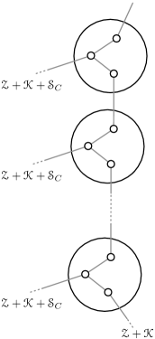
(a) This case occurs when the last star in the subsequence of adjacent stars has only one extremity.

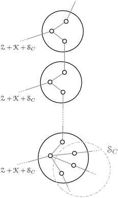
(b) This case occurs when the last star in the subsequence of adjacent stars has at least two extremities (here, it has three).

Figure 3: Combinatorial intuition behind the derivation of Appendix A.

The class ${\mathcal{DH}}_{\bullet}$ of distance-hereditary graphs rooted at a vertex is originally specified by

$${\mathcal{DH}}_{\bullet} =\mathcal{Z}_{\bullet}\times\left({\mathcal{K}}+{\mathcal{S}}_{C}+{\mathcal{S}}_{X}\right)$$

$${\mathcal{K}} ={\text{\sc Set}}_{\geqslant 2}\left(\mathcal{Z}+{\mathcal{S}}_{C}+{\mathcal{S}}_{X}\right)$$

$${\mathcal{S}}_{C} ={\text{\sc Set}}_{\geqslant 2}\left(\mathcal{Z}+{\mathcal{K}}+{\mathcal{S}}_{X}\right)$$

$${\mathcal{S}}_{X} =\left(\mathcal{Z}+{\mathcal{K}}+{\mathcal{S}}_{C}\right)\times{\text{\sc Set}}_{\geqslant 1}\left(\mathcal{Z}+{\mathcal{K}}+{\mathcal{S}}_{X}\right)\text{.}$$

The point of this appendix is to prove that the last equation can be simplified to

$${\mathcal{S}}_{X} ={\text{\sc Seq}}_{\geqslant 2}\left(\mathcal{Z}+{\mathcal{K}}+{\mathcal{S}}_{C}\right)\text{.}$$

Although we first provide a straightforward formal derivation, we then follow it up with an intuitive explanation.

Proof A.1.

Indeed, while the elements of a Set have symmetries that are hard to take into account, this is not the case for sets of size 1, therefore

$${\text{\sc Set}}_{\geqslant 1}\left({\mathcal{U}}\right)={\mathcal{U}}+{\text{\sc Set}}_{\geqslant 2}\left({\mathcal{U}}\right)\text{.}$$

By combining this fact with the definition of ${\mathcal{S}}_{C}$,

$${\mathcal{S}}_{C}={\text{\sc Set}}_{\geqslant 2}\left(\mathcal{Z}+{\mathcal{K}}+{\mathcal{S}}_{X}\right)\text{,}$$

we have that (parentheses in the right hand side purely for emphasis)

$${\text{\sc Set}}_{\geqslant 1}\left(\mathcal{Z}+{\mathcal{K}}+{\mathcal{S}}_{X}\right)\equiv\left(\mathcal{Z}+{\mathcal{K}}+{\mathcal{S}}_{X}\right)+{\mathcal{S}}_{C}$$

hence,

$${\mathcal{S}}_{X} =\left(\mathcal{Z}+{\mathcal{K}}+{\mathcal{S}}_{C}\right)\times\left(\mathcal{Z}+{\mathcal{K}}+{\mathcal{S}}_{X}+{\mathcal{S}}_{C}\right)$$

$$={\mathcal{S}}_{X}\times\left(\mathcal{Z}+{\mathcal{K}}+{\mathcal{S}}_{C}\right)+\left(\mathcal{Z}+{\mathcal{K}}+{\mathcal{S}}_{C}\right)^{2}$$

we then proceed to manipulate this specification purely symbolically, implying

$${\mathcal{S}}_{X}\left[1-\left(\mathcal{Z}+{\mathcal{K}}+{\mathcal{S}}_{C}\right)\right]=\left(\mathcal{Z}+{\mathcal{K}}+{\mathcal{S}}_{C}\right)^{2}$$

and thus

$${\mathcal{S}}_{X} =\frac{\left(\mathcal{Z}+{\mathcal{K}}+{\mathcal{S}}_{C}\right)^{2}}{1-\left(\mathcal{Z}+{\mathcal{K}}+{\mathcal{S}}_{C}\right)}$$

$$=\left(\mathcal{Z}+{\mathcal{K}}+{\mathcal{S}}_{C}\right)^{2}\times{\text{\sc Seq}}\left(\mathcal{Z}+{\mathcal{K}}+{\mathcal{S}}_{C}\right)$$

$$={\text{\sc Seq}}_{\geqslant 2}\left(\mathcal{Z}+{\mathcal{K}}+{\mathcal{S}}_{C}\right)\text{.}$$

Finally

$${\mathcal{S}}_{X}={\text{\sc Seq}}_{\geqslant 2}\left(\mathcal{Z}+{\mathcal{K}}+{\mathcal{S}}_{C}\right)\text{.}$$

Remark A.2.

To understand this simplification from a combinatorial perspective, imagine that we have a connected subsequence of star-nodes connected by their extremities.

Without loss of generality, we can assume that all but the last of these internal star-nodes have only two extremities—the one through which they are entered, and another one. We are then either in the situation illustrated by Figure 3 (in which the last star-node of the subsequence only has one additional extremity) or by Figure 3 (in which the last star-node has several extremities).

This subsequence of adjacent star-nodes connected by their extremities, translates to the grammar by a recursive expansion of the $\cramped{{\mathcal{S}}_{X}}$ rule: each of these has a $\cramped{(\mathcal{Z}+{\mathcal{K}}+{\mathcal{S}}_{C})}$ child for the center of the star, and then one other children for the other extremity. This is repeated until we have reached the last adjacent star-node in the subsequence which can either have one or multiple extremities:

• If it has only one extremity, then this extremity connects to either a leaf or to a clique, thus $\mathcal{Z}+{\mathcal{K}}$ (Figure 3).

• Otherwise, it has two or more undistinguished extremities, in which case we can pretend that this set of extremities is a $\cramped{{\mathcal{S}}_{C}}$ term (Figure 3).

Recall that the original interpretation of $\cramped{{\mathcal{S}}_{X}}$,

$${\mathcal{S}}_{X} =\left(\mathcal{Z}+{\mathcal{K}}+{\mathcal{S}}_{C}\right)\times{\text{\sc Set}}_{\geqslant 1}\left(\mathcal{Z}+{\mathcal{K}}+{\mathcal{S}}_{X}\right)\text{,}$$

is as follows: a distinguished center which can lead to either a leaf, a clique, or a star-node entered through its center; and a set of undistinguished extremities, each of which can lead to either a leaf, a clique, or another star-node entered through an extremity.

The new interpretation follows the figures: we have a sequence of $\cramped{(\mathcal{Z}+{\mathcal{K}}+{\mathcal{S}}_{C})}$ terms for the center of each of the adjacent star-nodes (and we have at least one such star-node), and finally another such term to cover both possibilities, where the final star-node either has one extremity or several. This is equivalent to having a sequence of at least two of these terms, hence the simplified equation.

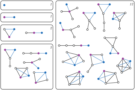
Figure 4: All unrooted, unlabeled 3-leaf power graphs of sizes 1 through 5, beginning the enumeration: 1, 1, 2, 5, 12, …. The coloring of the vertices illustrate one possible way to derive the graphs through vertex incremental operations sketched in Section 5: the newly added vertex is in blue, while the existing vertex it is added in reference to is in purple.

References

- [1] François Bergeron, Gilbert Labelle, and Pierre Leroux. Combinatorial Species and Tree-like Structures, volume 67 of Encyclopedia of Mathematics and Its Applications. Cambridge University Press, Cambridge, 1998.
- [2] Manuel Bodirsky, Éric Fusy, Mihyun Kang, and Stefan Vigerske. Enumeration and asymptotic properties of unlabeled outerplanar graphs. Electronic Journal of Combinatorics, 14(R66):1–24, 2007.
- [3] Manuel Bodirsky, Éric Fusy, Mihyun Kang, and Stefan Vigerske. Boltzmann samplers, Pólya theory, and cycle pointing. SIAM Journal on Computing, 40(3):721–769, 2011.
- [4] Binh-Minh Bui-Xuan. Tree-representation of set families in graph decompositions and efficient algorithms. PhD thesis, Université d’Orléans, 2008.
- [5] Guillaume Chapuy, Éric Fusy, Mihyun Kang, and Bilyana Shoilekova. A complete grammar for decomposing a family of graphs into 3-connected components. The Electronic Journal of Combinatorics, 15, 2008.
- [6] Pierre Charbit, Fabien de Montgolfier, and Mathieu Raffinot. Linear Time Split Decomposition Revisited. SIAM Journal on Discrete Mathematics, 26(2):499–514, 2012.
- [7] Cédric Chauve, Éric Fusy, and Jérémie Lumbroso. An Enumeration of Distance-Hereditary and 3-Leaf Power Graphs. Technical report, 2014. Preprint presented at ICGT 2014.
- [8] William H. Cunningham. Decomposition of Directed Graphs. SIAM Journal on Algebraic Discrete Methods, 3(2):214–228, 1982.
- [9] William H. Cunningham and Jack Edmonds. A combinatorial decomposition theory. Canadian Journal of Mathematics, 32(3):734–765, 1980.
- [10] Michael Drmota. Systems of Functional Equations. Random Structures & Algorithms, 10(1-2):103–124, 1997.
- [11] Michael Drmota. Trees. In Miklos Bona, editor, Handbook of Enumerative Combinatorics, pages 281–334. CRC Press, 2015.
- [12] Michael Drmota, Éric Fusy, Mihyun Kang, Veronika Kraus, and Juanjo Rué. Asymptotic Study of Subcritical Graph Classes. SIAM Journal on Discrete Mathematics, 25(4):1615–1651, 2011.
- [13] Philippe Duchon, Philippe Flajolet, Guy Louchard, and Gilles Schaeffer. Boltzmann Samplers for the Random Generation of Combinatorial Structures. Combinatorics, Probability and Computing, 13(4–5):577–625, 2004. Special issue on Analysis of Algorithms.
- [14] Philippe Flajolet, Éric Fusy, and Carine Pivoteau. Boltzmann Sampling of Unlabelled Structures. In David Applegate et al, editor, Proceedings of the Ninth Workshop on Algorithm Engineering and Experiments and the Fourth Workshop on Analytic Algorithmics and Combinatorics, pages 201–211. SIAM Press, 2007. Proceedings of the New Orleans Conference.
- [15] Philippe Flajolet and Bruno Salvy. Computer Algebra Libraries for Combinatorial Structures. Journal of Symbolic Computation, 20(5):653–671, 1995.
- [16] Philippe Flajolet and Robert Sedgewick. Analytic Combinatorics. Cambridge University Press, 2009.
- [17] Philippe Flajolet, Paul Zimmerman, and Bernard Van Cutsem. A Calculus for the Random Generation of Labelled Combinatorial Structures. Theoretical Computer Science, 132(1-2):1–35, 1994.
- [18] Omer Giménez and Marc Noy. Counting planar graphs and related families of graphs. Surveys in Combinatorics, 365:169–210, 2009.
- [19] Emeric Gioan and Christophe Paul. Split decomposition and graph-labelled trees: Characterizations and fully dynamic algorithms for totally decomposable graphs. Discrete Applied Mathematics, 160(6):708–733, 2012. Fourth Workshop on Graph Classes, Optimization, and Width Parameters Bergen, Norway, October 2009 Bergen (GROW) 09.
- [20] Emeric Gioan, Christophe Paul, Marc Tedder, and Derek G. Corneil. Practical and Efficient Split Decomposition via Graph-Labelled Trees. Algorithmica, pages 1–55, 2013.
- [21] Peter L. Hammer and Frédéric Maffray. Completely Separable Graphs. Discrete Applied Mathematics, 27(1):85–99, 1990.
- [22] Alexander Iriza. Enumeration and random generation of unlabeled classes of graphs: A practical study of cycle pointing and the dissymmetry theorem. Master’s thesis, Princeton University, arXiv preprint arXiv:1511.06037, 2015.
- [23] Shin-ichi Nakano, Ryuhei Uehara, and Takeaki Uno. A New Approach to Graph Recognition and Applications to Distance-Hereditary Graphs. Journal of Computer Science and Technology, 24(3):517–533, 2009.
- [24] Naomi Nishimura, Prabhakar Ragde, and Dimitrios M. Thilikos. On Graph Powers for Leaf-Labeled Trees. Journal of Algorithms, 42(1):69–108, 2002.
- [25] Vlady Ravelomanana and Loÿs Thimonier. Asymptotic enumeration of cographs. Electronic Notes in Discrete Mathematics, 7(0):58–61, 2001. Brazilian Symposium on Graphs, Algorithms and Combinatorics.
- [26] Jessica Shi. Enumeration of unlabeled graph classes: A study of tree decompositions and related approaches. 2015.
- [27] Jeremy P. Spinrad. Efficient Graph Representations, volume 19 of The Fields Institute for Research in Mathematical Sciences. American Mathematical Society, 2003.
- [28] Paul Zimmermann. Séries génératrices et analyse automatique d’algorithmes. PhD thesis, École Polytechnique, 1991.