Energy Conditions in $f(\mathcal{G},T)$ Gravity

Abstract

The aim of this paper is to introduce a new modified gravity theory named as $f(\mathcal{G},T)$ gravity ($\mathcal{G}$ and $T$ are the Gauss-Bonnet invariant and trace of the energy-momentum tensor, respectively) and investigate energy conditions for two reconstructed models in the context of FRW universe. We formulate general field equations, divergence of energy-momentum tensor, equation of motion for test particles as well as corresponding energy conditions. The massive test particles follow non-geodesic lines of geometry due to the presence of extra force. We express energy conditions in terms of cosmological parameters like deceleration, jerk and snap parameters. The reconstruction technique is applied to this theory using de Sitter and power-law cosmological solutions. We analyze energy bounds and obtain feasible constraints on free parameters.

Keywords: $f(\mathcal{G},T)$ gravity; Raychaudhuri equations; Energy conditions.
PACS: 04.50.Kd; 98.80.-k; 98.80.Jk.

1 Introduction

Current cosmic accelerated expansion has been affirmed from a diverse set of observational data coming from several astronomical evidences including supernova type Ia, large scale structure, cosmic microwave background radiation etc [1]. This expanding paradigm is considered as a consequence of mysterious force dubbed as dark energy (DE) which possesses negatively large pressure. Modified theories of gravity are considered as the favorite candidates to unveil the enigmatic nature of this energy. These modified theories are usually developed by including scalar invariants and their corresponding generic functions in the Einstein-Hilbert action.

A remarkably interesting gravity theory is the modified Gauss-Bonnet (GB) theory. A linear combination of the form

$$\mathcal{G}=R_{\alpha\beta\xi\eta}R^{\alpha\beta\xi\eta}-4R_{\alpha\beta}R^{\alpha\beta}+R^{2},$$

where $R_{\alpha\beta\xi\eta},~{}R_{\alpha\beta}$ and $R$ represent the Riemann tensor, Ricci tensor and Ricci scalar, respectively is called a Gauss-Bonnet invariant $(\mathcal{G})$. It is a second order Lovelock scalar invariant and thus free from spin-2 ghosts instabilities [2]. Gauss-Bonnet combination is a four-dimensional topological invariant which does not involve in the field equations. However, it provides interesting results in same dimensions when either coupled with scalar field or arbitrary function $f(\mathcal{G})$ is added to Einstein-Hilbert action [3]. The latter approach is introduced by Nojiri and Odintsov known as $f(\mathcal{G})$ theory of gravity [4]. Like other modified theories, this theory is an alternative to study DE and is consistent with solar system constraints [5]. In this context, there is a possibility to discuss a transition from decelerated to accelerated as well as from non-phantom to phantom phases and also to explain the unification of early and late times accelerated expansion of the universe [6].

The fascinating problem of cosmic accelerated expansion has successfully been discussed by taking into account modified theories of gravity with curvature matter coupling. The motion of test particles is studied in $f(R)$ and $f(\mathcal{G})$ gravity theories non-minimally coupled with matter Lagrangian density $(\mathcal{L}_{m})$. Consequently, the extra force experienced by test particles is found to be orthogonal to their four velocities and the motion becomes non-geodesic [7]. It is found that for certain choices of $\mathcal{L}_{m}$, the presence of extra force vanishes in non-minimal $f(R)$ model while it remains preserved in non-minimal $f(\mathcal{G})$ model. The geodesic deviation is weaker in $f(\mathcal{G})$ gravity for small curvatures as compared to non-minimal $f(R)$ gravity. Nojiri et al. [8] studied the non-minimally coupling of $f(R)$ and $f(\mathcal{G})$ theories with $\mathcal{L}_{m}$ and found that such coupling naturally unifies the inflationary era with current cosmic accelerated expansion.

In order to describe some realistic matter distribution, certain conditions must be imposed on the energy-momentum tensor ($T_{\alpha\beta}$) known as energy conditions. These conditions originate from Raychaudhuri equations with the requirement that not only the gravity is attractive but also the energy density is positive. The null (NEC), weak (WEC), dominant (DEC) and strong (SEC) energy conditions are the four fundamental conditions. They play a key role to study the theorems related to singularity and black hole thermodynamics. Null energy condition is important to discuss the second law of black hole thermodynamics while its violation leads to Big-Rip singularity of the universe [9]. The proof of positive mass theorem is based on DEC [10] while SEC is useful to study Hawking-Penrose singularity theorem [11].

Energy conditions have been investigated in different modified theories of gravity like $f(R)$ gravity, Brans-Dicke theory, $f(\mathcal{G})$ gravity, generalized teleparallel theory [12]. Banijamali et al. [13] investigated energy conditions for non-minimally coupling $f(\mathcal{G})$ theory with $\mathcal{L}_{m}$ and found that WEC is satisfied for specific viable $f(\mathcal{G})$ models. Sharif and Waheed [14] explored energy bounds in the context of generalized second order scalar-tensor gravity with the help of power-law ansatz for scalar field. Sharif and Zubair [15] derived these conditions in $f(R,T,R_{\alpha\beta}T^{\alpha\beta})$ theory of gravity for two specific models and also examined Dolgov-Kowasaki instability for particular models of $f(R,T)$ gravity.

In this paper, we introduce a new modified theory of gravity named as $f(\mathcal{G},T)$ gravity in which gravitational Lagrangian is obtained by adding a generic function $f(\mathcal{G},T)$ in the Einstein-Hilbert action. We study energy conditions for the reconstructed $f(\mathcal{G},T)$ models using isotropic homogeneous universe model. The paper has the following format. In section 2, we formulate the field equations of this gravity and discuss the equation of motion for test particles while general expressions for energy conditions as well as in terms of cosmological parameters are discussed in section 3. The reconstruction of models and their energy bounds are analyzed in section 4. In the last section, we summarize our results.

2 Field Equations of $f(\mathcal{G},T)$ Gravity

In this section, we formulate the field equations for $f(\mathcal{G},T)$ gravity. For this purpose, we assume action of the following form

$$\mathcal{S}=\frac{1}{2\kappa^{2}}\int d^{4}x\sqrt{-g}[R+f(\mathcal{G},T)]+\int d^{4}{x}\sqrt{-g}\mathcal{L}_{m},$$ (1)

where $g$ and $\kappa$ represent determinant of the metric tensor $(g_{\alpha\beta})$ and coupling constant, respectively. The energy-momentum tensor is defined as [16]

$$T_{\alpha\beta}=-\frac{2}{\sqrt{-g}}\frac{\delta(\sqrt{-g}\mathcal{L}_{m})}{\delta g^{\alpha\beta}}.$$ (2)

Assuming that the matter distribution depends on the components of $g_{\alpha\beta}$ but has no dependence on its derivatives, we obtain

$$T_{\alpha\beta}=g_{\alpha\beta}\mathcal{L}_{m}-2\frac{\partial\mathcal{L}_{m}}{\partial g^{\alpha\beta}}.$$ (3)

The variation in the action (1) gives

$$0 = \delta\mathcal{S}=\frac{1}{2\kappa^{2}}\int d^{4}x[(R+f(\mathcal{G},T))\delta\sqrt{-g}+\sqrt{-g}(\delta R+f_{\mathcal{G}}(\mathcal{G},T)\delta\mathcal{G}$$ (4)

$$+ f_{T}(\mathcal{G},T)\delta T)]+\int d^{4}x\delta(\sqrt{-g}\mathcal{L}_{m}),$$

where $f_{\mathcal{G}}(\mathcal{G},T)=\frac{\partial f(\mathcal{G},T)}{\partial\mathcal{G}}$ and $f_{T}(\mathcal{G},T)=\frac{\partial f(\mathcal{G},T)}{\partial T}$. The variation of $\sqrt{-g},\\ ~{}R^{\xi}_{\alpha\beta\eta},~{}R_{\alpha\eta}$ and $R$ provide the following expressions

$$\delta\sqrt{-g} = -\frac{1}{2}\sqrt{-g}g_{\alpha\beta}\delta g^{\alpha\beta},$$

$$\delta R^{\xi}_{\alpha\beta\eta} = \nabla_{\beta}(\delta\Gamma^{\xi}_{\eta\alpha})-\nabla_{\eta}(\delta\Gamma^{\xi}_{\beta\alpha}),$$

$$= (g_{\alpha\lambda}\nabla_{[\eta}\nabla_{\beta]}+g_{\lambda[\beta}\nabla_{\eta]}\nabla_{\alpha})\delta g^{\xi\lambda}+\nabla_{[\eta}\nabla^{\xi}\delta g_{\beta]\alpha},$$

$$\delta R_{\alpha\eta} = \delta R^{\xi}_{\alpha\xi\eta},\quad\delta R=(R_{\alpha\beta}+g_{\alpha\beta}\nabla^{2}-\nabla_{\alpha}\nabla_{\beta})\delta g^{\alpha\beta},$$ (5)

where $\Gamma^{\xi}_{\alpha\beta}$ and $\nabla_{\alpha}$ represent the Christoffel symbol and covariant derivative, respectively. The variation of $\mathcal{G}$ and $T$ yield

$$\delta\mathcal{G} = 2R\delta R-4\delta(R_{\alpha\beta}R^{\alpha\beta})+\delta(R_{\alpha\beta\xi\eta}R^{\alpha\beta\xi\eta}),$$

$$\delta T = (T_{\alpha\beta}+\Theta_{\alpha\beta})\delta g^{\alpha\beta},\quad\Theta_{\alpha\beta}=g^{\xi\eta}\frac{\delta T_{\xi\eta}}{\delta g_{\alpha\beta}}.$$ (6)

Using these variational relations in Eq.(4), we obtain the field equations of $f(\mathcal{G},T)$ gravity after simplification as follows

$$G_{\alpha\beta} = \kappa^{2}T_{\alpha\beta}-(T_{\alpha\beta}+\Theta_{\alpha\beta})f_{T}(\mathcal{G},T)+\frac{1}{2}g_{\alpha\beta}f(\mathcal{G},T)-(2RR_{\alpha\beta}-4R_{\alpha}^{\xi}R_{\xi\beta}$$ (7)

$$- 4R_{\alpha\xi\beta\eta}R^{\xi\eta}+2R_{\alpha}^{\xi\eta\delta}R_{\beta\xi\eta\delta})f_{\mathcal{G}}(\mathcal{G},T)-(2Rg_{\alpha\beta}\nabla^{2}-2R\nabla_{\alpha}\nabla_{\beta}$$

$$- 4g_{\alpha\beta}R^{\xi\eta}\nabla_{\xi}\nabla_{\eta}-4R_{\alpha\beta}\nabla^{2}+4R_{\alpha}^{\xi}\nabla_{\beta}\nabla_{\xi}+4R_{\beta}^{\xi}\nabla_{\alpha}\nabla_{\xi}$$

$$+ 4R_{\alpha\xi\beta\eta}\nabla^{\xi}\nabla^{\eta})f_{\mathcal{G}}(\mathcal{G},T),$$

where $G_{\alpha\beta}=R_{\alpha\beta}-\frac{1}{2}g_{\alpha\beta}R$ and $\nabla^{2}=\Box=\nabla_{\alpha}\nabla^{\alpha}$ denote the Einstein tensor and d’Alembert operator, respectively. It is worth mentioning here that for $f(\mathcal{G},T)=f(\mathcal{G})$, Eq.(7) reduces to the field equations for $f(\mathcal{G})$ gravity while $\Lambda(T)$ gravity ($\Lambda$ is the cosmological constant) is obtained in the absence of quadratic invariant $\mathcal{G}$ [4, 17]. Furthermore, the Einstein field equations are recovered when $f(\mathcal{G},T)=0$. The trace of Eq.(7) is given by

$$R+\kappa^{2}T-(T+\Theta)f_{T}(\mathcal{G},T)+2f(\mathcal{G},T)+2\mathcal{G}f_{\mathcal{G}}(\mathcal{G},T)-2R\nabla^{2}f_{\mathcal{G}}(\mathcal{G},T)$$

$$+ 4R^{\alpha\beta}\nabla_{\alpha}\nabla_{\beta}f_{\mathcal{G}}(\mathcal{G},T)=0,$$

where $\Theta=\Theta^{\alpha}_{\alpha}$. In this theory, the covariant divergence of Eq.(7) is non-zero given by

$$\nabla^{\alpha}T_{\alpha\beta} = \frac{f_{T}(\mathcal{G},T)}{\kappa^{2}-f_{T}(\mathcal{G},T)}\left[(T_{\alpha\beta}+\Theta_{\alpha\beta})\nabla^{\alpha}(\ln{f_{T}(\mathcal{G},T)})+\nabla^{\alpha}\Theta_{\alpha\beta}\right.$$ (8)

$$- \left.\frac{1}{2}g_{\alpha\beta}\nabla^{\alpha}T\right].$$

To obtain a useful expression for $\Theta_{\alpha\beta}$, we differentiate Eq.(3) with respect to metric tensor

$$\frac{\delta T_{\alpha\beta}}{\delta g^{\xi\eta}}=\frac{\delta g_{\alpha\beta}}{\delta g^{\xi\eta}}\mathcal{L}_{m}+g_{\alpha\beta}\frac{\partial\mathcal{L}_{m}}{\partial g^{\xi\eta}}-2\frac{\partial^{2}\mathcal{L}_{m}}{\partial g^{\xi\eta}\partial g^{\alpha\beta}}.$$ (9)

Using the relations

$$\frac{\delta g_{\alpha\beta}}{\delta g^{\xi\eta}}=-g_{\alpha\mu}g_{\beta\nu}\delta_{\xi\eta}^{\mu\nu},\quad\delta_{\xi\eta}^{\mu\nu}=\frac{\delta g^{\mu\nu}}{\delta g^{\xi\eta}},$$

where $\delta_{\xi\eta}^{\mu\nu}$ is the generalized Kronecker symbol and Eq.(9) in (6), we obtain

$$\Theta_{\alpha\beta}=-2T_{\alpha\beta}+g_{\alpha\beta}\mathcal{L}_{m}-2g^{\xi\eta}\frac{\partial^{2}\mathcal{L}_{m}}{\partial g^{\alpha\beta}\partial g^{\xi\eta}}.$$ (10)

This shows that once the value of $\mathcal{L}_{m}$ is determined, we can find the expression for tensor $\Theta_{\alpha\beta}$.

We consider matter distribution as the perfect fluid given by

$$T_{\alpha\beta}=(\rho+P)V_{\alpha}V_{\beta}-Pg_{\alpha\beta},$$ (11)

where $\rho,~{}P$ and $V_{\alpha}$ are the density, pressure and four velocity of the fluid, respectively. The four velocity satisfies the relation $V_{\alpha}V^{\alpha}=1$ and the corresponding Lagrangian density can be taken as $\mathcal{L}_{m}=-P$ [18]. Thus Eq.(10) yields

$$\Theta_{\alpha\beta}=-2T_{\alpha\beta}-Pg_{\alpha\beta}.$$ (12)

Equation (7) can be written in identical form to Einstein field equations as

$$G_{\alpha\beta}=\kappa^{2}T_{\alpha\beta}^{(eff)}=\kappa^{2}(T_{\alpha\beta}+T_{\alpha\beta}^{\mathcal{G}T}),$$ (13)

where $T_{\alpha\beta}^{\mathcal{G}T}$ is the $f(\mathcal{G},T)$ contribution. For the case of perfect fluid, the expression for $T_{\alpha\beta}^{\mathcal{G}T}$ is given by

$$T_{\alpha\beta}^{\mathcal{G}T} = \frac{1}{\kappa^{2}}\left[(\rho+P)V_{\alpha}V_{\beta}f_{T}(\mathcal{G},T)+\frac{1}{2}g_{\alpha\beta}f(\mathcal{G},T)-(2RR_{\alpha\beta}-4R_{\alpha}^{\xi}R_{\xi\beta}\right.$$ (14)

$$- \left.4R_{\alpha\xi\beta\eta}R^{\xi\eta}+2R_{\alpha}^{\xi\eta\delta}R_{\beta\xi\eta\delta})f_{\mathcal{G}}(\mathcal{G},T)-(2Rg_{\alpha\beta}\nabla^{2}-2R\nabla_{\alpha}\nabla_{\beta}\right.$$

$$- \left.4g_{\alpha\beta}R^{\xi\eta}\nabla_{\xi}\nabla_{\eta}-4R_{\alpha\beta}\nabla^{2}+4R_{\alpha}^{\xi}\nabla_{\beta}\nabla_{\xi}+4R_{\beta}^{\xi}\nabla_{\alpha}\nabla_{\xi}\right.$$

$$+ \left.4R_{\alpha\xi\beta\eta}\nabla^{\xi}\nabla^{\eta})f_{\mathcal{G}}(\mathcal{G},T)\right].$$

The line element for FRW universe model is

$$ds^{2}=dt^{2}-a^{2}(t)(dx^{2}+dy^{2}+dz^{2}),$$ (15)

where $a(t)$ represents the scale factor. The corresponding field equations are

$$3H^{2}=\kappa^{2}\rho_{eff},\quad-(2\dot{H}+3H^{2})=\kappa^{2}P_{eff},$$ (16)

where

$$\rho_{eff} = \rho+\frac{1}{\kappa^{2}}\left[(\rho+P)f_{T}(\mathcal{G},T)+\frac{1}{2}f(\mathcal{G},T)-12H^{2}(H^{2}+\dot{H})f_{\mathcal{G}}(\mathcal{G},T)\right.$$ (17)

$$+ \left.12H^{3}\partial_{t}f_{\mathcal{G}}(\mathcal{G},T)\right],$$

$$P_{eff} = P-\frac{1}{\kappa^{2}}\left[\frac{1}{2}f(\mathcal{G},T)-12H^{2}(H^{2}+\dot{H})f_{\mathcal{G}}(\mathcal{G},T)+8H(H^{2}+\dot{H})\right.$$ (18)

$$\times \left.\partial_{t}f_{\mathcal{G}}(\mathcal{G},T)+4H^{2}\partial_{tt}f_{\mathcal{G}}(\mathcal{G},T)\right],$$

$\mathcal{G}=24H^{2}(H^{2}+\dot{H})$, $H=\dot{a}/a$ is the Hubble parameter and dot represents the time derivative. The divergence of $T_{\alpha\beta}$ takes the form

$$\dot{\rho}+3H(\rho+P)=\frac{-1}{\kappa^{2}+f_{T}(\mathcal{G},T)}\left[\left(\dot{P}+\frac{1}{2}\dot{T}\right)f_{T}(\mathcal{G},T)+(\rho+P)\partial_{t}f_{T}(\mathcal{G},T)\right].$$ (19)

To obtain standard conservation equation

$$\dot{\rho}+3H(\rho+P)=0,$$ (20)

we need an additional constraint by taking the right side of Eq.(19) equal to zero given by

$$\left(\dot{P}+\frac{1}{2}\dot{T}\right)f_{T}(\mathcal{G},T)+(\rho+P)\partial_{t}f_{T}(\mathcal{G},T)=0.$$ (21)

Now, we briefly discuss the motion of test particles in $f(\mathcal{G},T)$ gravity. For this purpose, using Eqs.(11) and (12) in (8), the divergence of energy-momentum tensor for perfect fluid is given by

$$\nabla_{\beta}(\rho+P)V^{\alpha}V^{\beta}+(\rho+P)[V^{\beta}\nabla_{\beta}V^{\alpha}+V^{\alpha}\nabla_{\beta}V^{\beta}]-g^{\alpha\beta}\nabla_{\beta}P$$

$$=\frac{-2}{2\kappa^{2}+3f_{T}(\mathcal{G},T)}\left[T^{\alpha\beta}\nabla_{\beta}f_{T}(\mathcal{G},T)+g^{\alpha\beta}\nabla_{\beta}(Pf_{T}(\mathcal{G},T))\right].$$

The contraction of above equation with projection operator $(h_{\alpha\xi}=g_{\alpha\xi}-V_{\alpha\xi})$ gives the following expression

$$g_{\alpha\xi}V^{\beta}\nabla_{\beta}V^{\alpha}=\frac{(2\kappa^{2}+f_{T}(\mathcal{G},T))\nabla_{\beta}}{(\rho+P)(2\kappa^{2}+3f_{T}(\mathcal{G},T))}h_{\xi}^{\beta},$$ (22)

where we have used the relations $V^{\alpha}\nabla_{\beta}V_{\alpha}=0,~{}h_{\alpha\xi}V^{\alpha}=0$ and $h_{\alpha\xi}T^{\alpha\beta}=-Ph_{\xi}^{\beta}$. Multiplying Eq.(22) with $g^{\mu\xi}$ and using the following identity [18]

$$V^{\beta}\nabla_{\beta}V^{\alpha}=\frac{d^{2}x^{\alpha}}{ds^{2}}+\Gamma^{\alpha}_{\beta\xi}V^{\beta}V^{\xi},$$

we obtain the equation of motion for massive test particles in this gravity as

$$\frac{d^{2}x^{\alpha}}{ds^{2}}+\Gamma^{\alpha}_{\beta\xi}V^{\beta}V^{\xi}=\zeta^{\alpha},$$ (23)

where

$$\zeta^{\alpha}=\frac{(2\kappa^{2}+f_{T}(\mathcal{G},T))}{(\rho+P)(2\kappa^{2}+3f_{T}(\mathcal{G},T))}(g^{\alpha\beta}-V^{\alpha}V^{\beta})\nabla_{\beta}P,$$ (24)

represents the extra force acting on the test particles and is perpendicular to the four velocity of the fluid ($\zeta^{\alpha}V_{\alpha}=0$). For pressureless fluid, Eq.(24) gives $\zeta^{\alpha}=0$ and hence the dust particles follow the geodesic trajectories both in general relativity as well as in $f(\mathcal{G},T)$ gravity. The equation of motion for perfect fluid in general relativity is recovered in the absence of coupling between matter and geometry [19].

3 Energy Conditions

Energy conditions are the coordinate invariant which incorporate the common characteristics shared by almost every matter field. The concept of energy conditions came from the Raychaudhuri equations which play a key role to discuss the congruence of null and timelike geodesics with the requirement that not only the gravity is attractive but also the energy density is positive. These equations describe the temporal evolution of expansion scalar $(\theta)$ as follows [20]

$$\frac{d\theta}{d\tau} = -\frac{1}{3}\theta^{2}+\omega_{\alpha\beta}\omega^{\alpha\beta}-\sigma_{\alpha\beta}\sigma^{\alpha\beta}-R_{\alpha\beta}u^{\alpha}u^{\beta},$$ (25)

$$\frac{d\theta}{d\tau} = -\frac{1}{2}\theta^{2}+\omega_{\alpha\beta}\omega^{\alpha\beta}-\sigma_{\alpha\beta}\sigma^{\alpha\beta}-R_{\alpha\beta}k^{\alpha}k^{\beta},$$ (26)

where $\omega_{\alpha\beta},~{}\sigma_{\alpha\beta},~{}u^{\alpha}$ and $k^{\alpha}$ represent the rotation, shear tensor, timelike and null tangent vectors in the congruences, respectively. For non-geodesic congruences, the temporal evolution of $\theta$ is affected by the presence of acceleration term which arises due to non-gravitational force like pressure gradient as [21]

$$\frac{d\theta}{d\tau}=-\frac{1}{3}\theta^{2}+\omega_{\alpha\beta}\omega^{\alpha\beta}-\sigma_{\alpha\beta}\sigma^{\alpha\beta}+\nabla_{\alpha}(V^{\beta}\nabla_{\beta}V^{\alpha})-R_{\alpha\beta}V^{\alpha}V^{\beta}.$$ (27)

Neglecting the quadratic terms due to rotation-free as well as small distortions described by $\sigma_{\alpha\beta}$, Eqs.(25) and (26) yield

$$\theta=-\tau R_{\alpha\beta}u^{\alpha}u^{\beta},\quad\theta=-\tau R_{\alpha\beta}k^{\alpha}k^{\beta}.$$

Using the condition for gravity to be attractive, i.e., $\theta<0$, we obtain $R_{\alpha\beta}u^{\alpha}u^{\beta}\geq 0$ and $R_{\alpha\beta}k^{\alpha}k^{\beta}\geq 0$. The equivalent form of these inequalities can be obtained by the inversion of the Einstein field equations as

$$\left(T_{\alpha\beta}-\frac{1}{2}g_{\alpha\beta}T\right)u^{\alpha}u^{\beta}\geq 0,\quad\left(T_{\alpha\beta}-\frac{1}{2}g_{\alpha\beta}T\right)k^{\alpha}k^{\beta}\geq 0.$$

For perfect fluid matter distribution, these inequalities provide the energy constraints defined by

• NEC:$\quad\rho+P\geq 0$,

• WEC:$\quad\rho+P\geq 0,\quad\rho\geq 0,$

• SEC:$\quad\rho+P\geq 0,\quad\rho+3P\geq 0,$

• DEC:$\quad\rho\pm P\geq 0,\quad\rho\geq 0.$

These conditions show that the violation of NEC leads to the violation of all other conditions. Due to purely geometric nature of Raychaudhuri equations, the concept of energy bounds in modified theories of gravity can be extended with the assumption that the total cosmic matter distribution acts like a perfect fluid. The energy conditions can be formulated by replacing $\rho$ and $P$ with $\rho_{eff}$ and $P_{eff}$, respectively. The geodesic lines of geometry are followed by dust particles in $f(\mathcal{G},T)$ gravity, therefore we consider pressureless fluid to discuss the energy conditions. These conditions take the following form

$$\textbf{NEC:}\quad\rho_{eff}+P_{eff}=\rho+\frac{1}{\kappa^{2}}\left[\rho f_{T}(\mathcal{G},T)+4H(H^{2}-2\dot{H})\partial_{t}f_{\mathcal{G}}(\mathcal{G},T)\right.$$

$$\left.-4H^{2}\partial_{tt}f_{\mathcal{G}}(\mathcal{G},T)\right]\geq 0,$$ (28)

$$\textbf{WEC:}\quad\rho_{eff}=\rho+\frac{1}{2\kappa^{2}}\left[2\rho f_{T}(\mathcal{G},T)+f(\mathcal{G},T)-24H^{2}(H^{2}+\dot{H})\right.$$

$$\left.\times f_{\mathcal{G}}(\mathcal{G},T)+24H^{3}\partial_{t}f_{\mathcal{G}}(\mathcal{G},T)\right]\geq 0,$$ (29)

$$\textbf{SEC:}\quad\rho_{eff}+3P_{eff}=\rho-\frac{1}{\kappa^{2}}\left[f(\mathcal{G},T)-\rho f_{T}(\mathcal{G},T)-24H^{2}(H^{2}+\dot{H})\right.$$

$$\left.\times f_{\mathcal{G}}(\mathcal{G},T)+12H(H^{2}+2\dot{H})\partial_{t}f_{\mathcal{G}}(\mathcal{G},T)+12H^{2}\partial_{tt}f_{\mathcal{G}}(\mathcal{G},T)\right]\geq 0,$$ (30)

$$\textbf{DEC:}\quad\rho_{eff}-P_{eff}=\rho+\frac{1}{\kappa^{2}}\left[\rho f_{T}(\mathcal{G},T)+f(\mathcal{G},T)-24H^{2}(H^{2}+\dot{H})\right.$$

$$\left.\times f_{\mathcal{G}}(\mathcal{G},T)+4H(5H^{2}+2\dot{H})\partial_{t}f_{\mathcal{G}}(\mathcal{G},T)+4H^{2}\partial_{tt}f_{\mathcal{G}}(\mathcal{G},T)\right]\geq 0.$$ (31)

The Hubble parameter, Ricci scalar, GB invariant and their derivatives can be written in terms of cosmic parameters as

$$\dot{H} = -H^{2}(1+q),\quad\ddot{H}=H^{3}(j+3q+2),$$

$$\dddot{H} = H^{4}(s-4j-3q^{2}-12q-6),$$ (32)

$$R = -6H^{2}(1-q),\quad\dot{R}=-6H^{3}(j-q-2),$$

$$\ddot{R} = -6H^{4}(s+8q+q^{2}+6),$$ (33)

$$\mathcal{G} = -24qH^{4},\quad\dot{\mathcal{G}}=24H^{5}(j+3q+2q^{2}),$$

$$\ddot{\mathcal{G}} = 24H^{6}(s-6j-6qj-12q-15q^{2}-2q^{3}),$$ (34)

where $q,~{}j$ and $s$ denote the deceleration, jerk and snap parameters, respectively and are defined as [22]

$$q=-\frac{1}{H^{2}}\frac{\ddot{a}}{a},\quad j=\frac{1}{H^{3}}\frac{\dddot{a}}{a},\quad s=\frac{1}{H^{4}}\frac{\ddddot{a}}{a}.$$ (35)

The energy conditions (28)-(31) in the form of above parameters are

$$\textbf{NEC:}\quad\rho_{eff}+P_{eff}=\rho+\frac{1}{\kappa^{2}}\left[\rho f_{T}+4H^{3}(3+2q)(f_{\mathcal{GG}}\dot{\mathcal{G}}+f_{\mathcal{G}T}\dot{T})\right.$$

$$\left.-4H^{2}(f_{\mathcal{GGG}}\dot{\mathcal{G}}^{2}+2f_{\mathcal{GG}T}\dot{\mathcal{G}}\dot{T}+f_{\mathcal{G}TT}\dot{T}^{2}+f_{\mathcal{GG}}\ddot{\mathcal{G}}+f_{\mathcal{G}T}\ddot{T})\right]\geq 0,$$ (36)

$$\textbf{WEC:}\quad\rho_{eff}=\rho+\frac{1}{2\kappa^{2}}\left[f+2\rho f_{T}+24qH^{4}f_{\mathcal{G}}+24H^{3}(f_{\mathcal{GG}}\dot{\mathcal{G}}\right.$$

$$\left.+f_{\mathcal{G}T}\dot{T})\right]\geq 0,$$ (37)

$$\textbf{SEC:}\quad\rho_{eff}+3P_{eff}=\rho+\frac{1}{\kappa^{2}}\left[-f+\rho f_{T}-24qH^{4}f_{\mathcal{G}}+12H^{3}(1+2q)\right.$$

$$\left.\times(f_{\mathcal{GG}}\dot{\mathcal{G}}+f_{\mathcal{G}T}\dot{T})-12H^{2}(f_{\mathcal{GGG}}\dot{\mathcal{G}}^{2}+2f_{\mathcal{GG}T}\dot{\mathcal{G}}\dot{T}+f_{\mathcal{G}TT}\dot{T}^{2}+f_{\mathcal{GG}}\ddot{\mathcal{G}}\right.$$

$$\left.+f_{\mathcal{G}T}\ddot{T})\right]\geq 0,$$ (38)

$$\textbf{DEC:}\quad\rho_{eff}-P_{eff}=\rho+\frac{1}{\kappa^{2}}\left[f+\rho f_{T}+24qH^{4}f_{\mathcal{G}}+4H^{3}(3-2q)(f_{\mathcal{GG}}\dot{\mathcal{G}}\right.$$

$$\left.+f_{\mathcal{G}T}\dot{T})+4H^{2}(f_{\mathcal{GGG}}\dot{\mathcal{G}}^{2}+2f_{\mathcal{GG}T}\dot{\mathcal{G}}\dot{T}+f_{\mathcal{G}TT}\dot{T}^{2}+f_{\mathcal{GG}}\ddot{\mathcal{G}}+f_{\mathcal{G}T}\ddot{T})\right]\geq 0.$$ (39)

4 Reconstruction of $f(\mathcal{G},T)$ Models

In this section, we use the reconstruction technique and discuss the energy conditions for de Sitter and power-law universe models.

4.1 de Sitter Universe Model

This cosmological model explains the exponential expansion of the universe with constant Hubble expansion rate. The scale factor is defined as [23]

$$a(t)=a_{0}e^{H_{0}t},\quad H=H_{0},$$ (40)

where $a_{0}$ is constant at $t_{0}$. The values of $R$ and GB invariant are

$$R=-12H_{0}^{2},\quad\mathcal{G}=24H_{0}^{4}.$$ (41)

For pressureless fluid, Eq.(20) gives the energy density of the form

$$\rho=\rho_{0}e^{-3H_{0}t}.$$ (42)

The trace of energy-momentum tensor and its derivatives have the following expressions

$$T=\rho,\quad\dot{T}=-3H_{0}T,\quad\ddot{T}=9H_{0}^{2}T.$$ (43)

Using Eqs.(40)-(43) in Eq.(16), we obtain partial differential equation

$$\kappa^{2}T+\frac{1}{2}f(\mathcal{G},T)-12H_{0}^{4}f_{\mathcal{G}}(\mathcal{G},T)+Tf_{T}(\mathcal{G},T)-36H_{0}^{4}T{f_{\mathcal{G}T}}(\mathcal{G},T)$$ (44)

$$- 3H_{0}^{2}=0,$$

whose solution is given by

$$f(\mathcal{G},T)=c_{1}c_{2}\left(e^{c_{1}\mathcal{G}}T^{\gamma_{1}}+T^{\gamma_{2}}\right)+\gamma_{3}T+\gamma_{4},$$ (45)

where $c_{i}$’s are integration constants and

$$\gamma_{1}=-\frac{1}{2}\left(\frac{1-24c_{1}H_{0}^{4}}{1-36c_{1}H_{0}^{4}}\right),\quad\gamma_{2}=-\frac{1}{2},\quad\gamma_{3}=-\frac{2}{3}\kappa^{2},\quad\gamma_{4}=6H_{0}^{2}.$$

The additional constraint (21) becomes

$$c_{1}c_{2}\frac{(1-24c_{1}H_{0}^{4})(1-30c_{1}H_{0}^{4})}{(1-36c_{1}H_{0}^{4})^{2}}e^{c_{1}\mathcal{G}}T^{\gamma_{1}}+c_{1}c_{2}T^{\gamma_{2}}+\gamma_{3}T=0.$$

This equation splits Eq.(45) into two $f(\mathcal{G},T)$ functions with some additional constant relations between the coefficients. The reconstructed model (45) can be written as a combination of those functions. We analyze the energy conditions for the $f(\mathcal{G},T)$ model given in Eq.(45) instead of analyzing them separately. Using model (45) in energy conditions (28)-(31), it follows that

$$\textbf{NEC:}\quad\rho_{eff}+P_{eff}=\rho+\frac{1}{\kappa^{2}}\left[\rho\left\{c_{1}c_{2}(\gamma_{1}e^{c_{1}\mathcal{G}}T^{(\gamma_{1}-1)}+\gamma_{2}T^{(\gamma_{2}-1)})+\gamma_{3}\right\}\right.$$

$$\left.+12c_{1}^{2}c_{2}\gamma_{1}H_{0}^{4}(1-3\gamma_{1})e^{c_{1}\mathcal{G}}T^{\gamma_{1}}\right]\geq 0,$$ (46)

$$\textbf{WEC:}\quad\rho_{eff}=\rho+\frac{1}{2\kappa^{2}}\left[2\rho\{c_{1}c_{2}(e^{c_{1}\mathcal{G}}\gamma_{1}T^{(\gamma_{1}-1)}+\gamma_{2}T^{(\gamma_{2}-1)})+\gamma_{3}\}\right.$$

$$\left.+\{c_{1}c_{2}(e^{c_{1}\mathcal{G}}T^{\gamma_{1}}+T^{\gamma_{2}})+\gamma_{3}T+\gamma_{4}\}-24c_{1}^{2}c_{2}H_{0}^{4}e^{c_{1}\mathcal{G}}T^{\gamma_{1}}(1+3\gamma_{1})\right]\geq 0,$$

(47)

$$\textbf{SEC:}\quad\rho_{eff}+3P_{eff}=\rho-\frac{1}{\kappa^{2}}\left[c_{1}c_{2}(e^{c_{1}\mathcal{G}}T^{\gamma_{1}}+T^{\gamma_{2}})+\gamma_{3}T+\gamma_{4}-\rho\right.$$

$$\left.\times\{c_{1}c_{2}\left(\gamma_{1}e^{c_{1}\mathcal{G}}T^{(\gamma_{1}-1)}+\gamma_{2}T^{(\gamma_{2}-1)}\right)+\gamma_{3}\}-12c_{1}^{2}c_{2}e^{c_{1}\mathcal{G}}H_{0}^{4}T^{\gamma_{1}}\right.$$

$$\left.\times\left\{2+3\gamma_{1}-9\gamma_{1}^{2}\right\}\right]\geq 0,$$ (48)

$$\textbf{DEC:}\quad\rho_{eff}-P_{eff}=\rho+\frac{1}{\kappa^{2}}[\rho\{c_{1}c_{2}(e^{c_{1}\mathcal{G}}\gamma_{1}T^{(\gamma_{1}-1)}+\gamma_{2}T^{(\gamma_{2}-1)})+\gamma_{3}\}$$

$$+\{c_{1}c_{2}(e^{c_{1}\mathcal{G}}T^{\gamma_{1}}+T^{\gamma_{2}})+\gamma_{3}T+\gamma_{4}\}-12c_{1}^{2}c_{2}H_{0}^{4}e^{c_{1}\mathcal{G}}T^{\gamma_{1}}$$

$$\times\{2+\gamma_{1}(5-3\gamma_{1})\}]\geq 0.$$ (49)

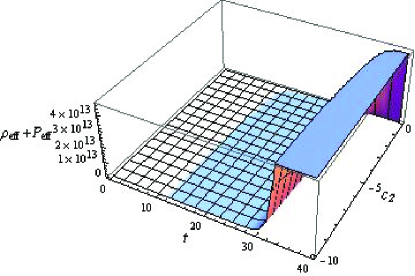
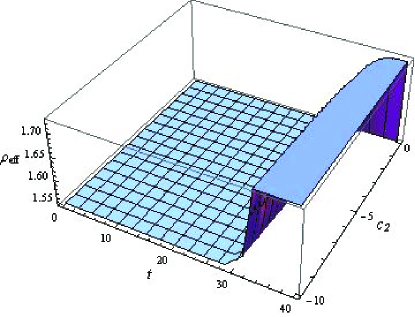
Figure 1: Energy conditions for $c_{1}=0.001$.

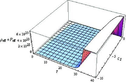
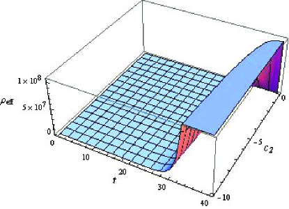
Figure 2: Energy conditions for $c_{1}=4$.

Figures 1 and 2 show the variation of NEC and WEC for the case $c_{1}>0$ and $c_{2}<0$ with $\kappa=1$. We use the following values of cosmological parameters: $H_{0}=0.718,~{}q=-0.64,~{}j=1.02$ and $s=-0.39$ [24]. In these plots, we fix the constant $c_{1}$ for two arbitrarily chosen values while $c_{2}$ varies from $[-10,0]$. Figure 1 shows the positively increasing behavior of NEC as well as WEC with respect to time in the considered interval of $c_{2}$. Figure 2 shows similar behavior for $c_{1}=4$. In this case, both conditions are satisfied for all values of $c_{1}$ and $c_{2}$. The energy conditions for $(c_{1},c_{2})>0$ are discussed in Figures 3 and 4. The left plot of Figure 3 shows that the NEC is satisfied for $t<3,~{}t<2.28$ and $t=2$ for $c_{2}=0.005,~{}0.05$ and $0.1$, respectively. Figure 4 (left) shows similar decreasing behavior of time as the value of $c_{2}$ increases for $c_{1}=0.01$. It is also observed that as the value of $c_{1}$ increases, the time interval for valid NEC decreases while the positivity of $\rho_{eff}$ is shown in the right panel of both figures. For the case $(c_{1},c_{2})>0$, both NEC and WEC are satisfied for small values of $c_{1}$ and $c_{2}$ in a very small time interval.

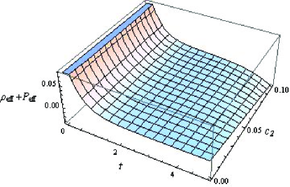
Figure 3: Energy conditions for $c_{1}=0.001$.

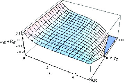
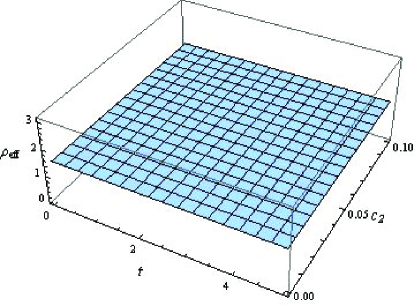
Figure 4: Energy conditions for $c_{1}=0.01$.

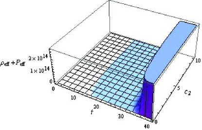
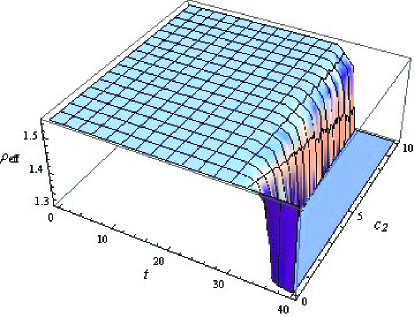
Figure 5: Energy conditions for $c_{1}=-0.01$.

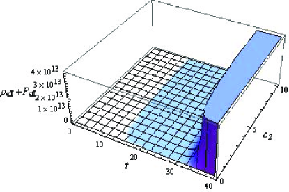
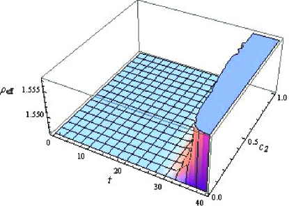
Figure 6: Energy conditions for $c_{1}=-0.001$.

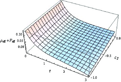
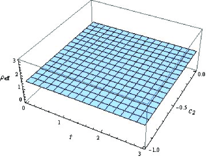
Figure 7: Energy conditions for $c_{1}=-0.001$.

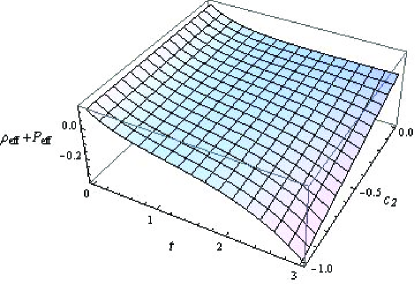
Figure 8: Energy conditions for $c_{1}=-0.01$.

Figures 5 and 6 deal with the case $c_{1}<0$ and $c_{2}>0$. For arbitrarily chosen values of $c_{1}$, the increasing behavior of NEC with respect to time is observed in the left panel of both figures for all values of $c_{2}$. The right plot of Figure 5 shows the positivity of $\rho_{eff}$ for $t<34$ while it remains positive throughout the time interval for $c_{1}=-0.001$ as shown in Figure 6 (right panel). The last possibility, i.e., $c_{1}<0$ and $c_{2}<0$ is examined in Figures 7 and 8. The left panel of both figures show the decreasing and increasing behavior of NEC as the time and integration constant $c_{2}$ increase, respectively. The effective energy density exhibits constant behavior for assumed values of $c_{1}$ in the considered interval of $c_{2}$.

4.2 Power-law Solution

The power-law solution is of great interest to discuss the cosmic evolution and its scale factor is defined as [23]

$$a(t)=a_{0}t^{n},\quad H=\frac{n}{t},$$ (50)

where $n>0$. For $0<n<1$, we have decelerated universe which leads to radiation dominated era for $n=\frac{1}{2}$ and dust dominated era for $n=\frac{2}{3}$ while cosmic accelerated era is observed for $n>1$. The Ricci scalar and GB invariant are

$$R=\frac{6n}{t^{2}}(1-2n),\quad\mathcal{G}=\frac{24n^{3}}{t^{4}}(n-1).$$ (51)

The energy density for dust fluid is obtained from Eq.(20) as

$$\rho=\rho_{0}t^{-3n}.$$ (52)

The trace of $T_{\alpha\beta}$ and its time derivatives take the form

$$T=\rho,\quad\dot{T}=-\frac{3n}{t}T,\quad\ddot{T}=\frac{3n}{t^{2}}(1+3n)T.$$ (53)

Inserting Eqs.(50)-(53) in the first field equation (16), we obtain

$$\kappa^{2}T+\frac{1}{2}f(\mathcal{G},T)-\frac{1}{2}\mathcal{G}f_{\mathcal{G}}(\mathcal{G},T)+Tf_{T}(\mathcal{G},T)-\left(\frac{2}{n-1}\right)\mathcal{G}^{2}f_{\mathcal{GG}}(\mathcal{G},T)$$ (54)

$$- \left(\frac{3n}{2(n-1)}\right)\mathcal{G}Tf_{\mathcal{G}T}(\mathcal{G},T)-3n^{2}\left(\frac{T}{\rho_{0}}\right)^{\frac{2}{3n}}=0,$$

whose solution is given by

$$f(\mathcal{G},T) = d_{1}d_{3}T^{d_{2}}\mathcal{G}^{\frac{1}{4}(\chi_{1}+\chi_{2})}+d_{2}d_{3}T^{d_{2}}\mathcal{G}^{-\frac{1}{4}(\chi_{1}-\chi_{2})}+\chi_{3}T$$ (55)

$$+ d_{1}d_{2}T^{\chi_{4}}+\chi_{5}T^{\chi_{6}},$$

where $d_{i}$’s are constants of integration and

$$\chi_{1} = \frac{1}{2}\left[n^{2}(1+3d_{2}(3d_{2}+2))+2d_{2}(n-16)+3(2n+3)\right]^{\frac{1}{2}},$$

$$\chi_{2} = \frac{1}{2}\left[5-n(1+3d_{2})\right],\quad\chi_{3}=-\frac{2}{3}\kappa^{2},\quad\chi_{4}=-\frac{1}{2},$$

$$\chi_{5} = \left(\frac{18n^{3}}{2+3n}\right)\rho_{0}^{-\frac{2}{3n}},\quad\chi_{6}=\frac{2}{3n}.$$

In this case, Eq.(21) takes the form

$$d_{1}d_{3}T^{d_{2}}\mathcal{G}^{\frac{1}{4}(\chi_{1}+\chi_{2})}\left[\frac{d_{2}}{6n}\{3n(2d_{2}-1)+2(\chi_{1}+\chi_{2})\}\right]+d_{2}d_{3}T^{d_{2}}\mathcal{G}^{-\frac{1}{4}(\chi_{1}-\chi_{2})}$$

$$\times \left[\frac{d_{2}}{6n}\{3n(2d_{2}-1)-2(\chi_{1}-\chi_{2})\}\right]+\chi_{3}T+d_{1}d_{2}\chi_{4}^{2}T^{\chi_{4}}+\chi_{5}\chi_{6}^{2}T^{\chi_{6}}=0.$$

Solving Eq.(55) with the above equation as in the previous section, we obtain two functions whose combination is equivalent to the reconstructed power-law $f(\mathcal{G},T)$ model.

Inserting the model (55) in energy conditions (36)-(39), we obtain

$$\textbf{NEC:}\quad\rho_{eff}+P_{eff}=\rho+\frac{1}{\kappa^{2}}\left[4H^{3}(3+2q)([\frac{1}{4}d_{1}d_{3}\right.$$

$$\left.\times(\chi_{1}+\chi_{2})\left[\frac{1}{4}(\chi_{1}+\chi_{2})-1\right]T^{d_{2}}\mathcal{G}^{\frac{1}{4}(\chi_{1}+\chi_{2})-2}+\frac{1}{4}d_{2}d_{3}(\chi_{1}-\chi_{2})\right.$$

$$\left.\times\left[\frac{1}{4}(\chi_{1}-\chi_{2})+1\right]T^{d_{2}}\mathcal{G}^{-\frac{1}{4}(\chi_{1}-\chi_{2})-2}]\dot{\mathcal{G}}+[\frac{1}{4}d_{1}d_{2}d_{3}(\chi_{1}+\chi_{2})T^{d_{2}-1}\right.$$

$$\left.\times\mathcal{G}^{\frac{1}{4}(\chi_{1}+\chi_{2})-1}-\frac{1}{4}d_{2}^{2}d_{3}(\chi_{1}-\chi_{2})T^{d_{2}-1}\mathcal{G}^{-\frac{1}{4}(\chi_{1}-\chi_{2})-1}]\dot{T})\right.$$

$$\left.-4H^{2}([\frac{1}{4}d_{1}d_{3}(\chi_{1}+\chi_{2})\left[\frac{1}{4}(\chi_{1}+\chi_{2})-1\right]\left[\frac{1}{4}(\chi_{1}+\chi_{2})-2\right]T^{d_{2}}\right.$$

$$\left.\times\mathcal{G}^{\frac{1}{4}(\chi_{1}+\chi_{2})-3}-\frac{1}{4}d_{2}d_{3}(\chi_{1}-\chi_{2})\left[\frac{1}{4}(\chi_{1}-\chi_{2})+1\right]\left[\frac{1}{4}(\chi_{1}-\chi_{2})+2\right]\right.$$

$$\left.\times T^{d_{2}}\mathcal{G}^{-\frac{1}{4}(\chi_{1}-\chi_{2})-3}]\dot{\mathcal{G}}^{2}+2[\frac{1}{4}d_{1}d_{2}d_{3}(\chi_{1}+\chi_{2})\left[\frac{1}{4}(\chi_{1}+\chi_{2})-1\right]T^{d_{2}-1}\right.$$

$$\left.\times\mathcal{G}^{\frac{1}{4}(\chi_{1}+\chi_{2})-2}+\frac{1}{4}d_{2}^{2}d_{3}(\chi_{1}-\chi_{2})\left[\frac{1}{4}(\chi_{1}-\chi_{2})+1\right]T^{d_{2}-1}\mathcal{G}^{-\frac{1}{4}(\chi_{1}-\chi_{2})-2}]\right.$$

$$\left.\times\dot{\mathcal{G}}\dot{T}+[\frac{1}{4}d_{1}d_{2}d_{3}(d_{2}-1)(\chi_{1}+\chi_{2})T^{d_{2}-2}\mathcal{G}^{\frac{1}{4}(\chi_{1}+\chi_{2})-1}-\frac{1}{4}d_{2}^{2}d_{3}(d_{2}-1)\right.$$

$$\left.\times(\chi_{1}-\chi_{2})T^{d_{2}-2}\mathcal{G}^{-\frac{1}{4}(\chi_{1}-\chi_{2})-1}]\dot{T}^{2}+[\frac{1}{4}d_{1}d_{3}(\chi_{1}+\chi_{2})\left[\frac{1}{4}(\chi_{1}+\chi_{2})-1\right]\right.$$

$$\left.\times T^{d_{2}}\mathcal{G}^{\frac{1}{4}(\chi_{1}+\chi_{2})-2}+\frac{1}{4}d_{2}d_{3}(\chi_{1}-\chi_{2})\left[\frac{1}{4}(\chi_{1}-\chi_{2})+1\right]T^{d_{2}}\mathcal{G}^{-\frac{1}{4}(\chi_{1}-\chi_{2})-2}]\right.$$

$$\left.\times\ddot{\mathcal{G}}+[\frac{1}{4}d_{1}d_{2}d_{3}(\chi_{1}+\chi_{2})T^{d_{2}-1}\mathcal{G}^{\frac{1}{4}(\chi_{1}+\chi_{2})-1}-\frac{1}{4}d_{2}^{2}d_{3}(\chi_{1}-\chi_{2})T^{d_{2}-1}\right.$$

$$\left.\times\mathcal{G}^{-\frac{1}{4}(\chi_{1}-\chi_{2})-1}]\ddot{T})+\rho[d_{1}d_{2}d_{3}T^{d_{2}-1}\mathcal{G}^{\frac{1}{4}(\chi_{1}+\chi_{2})}+d_{2}^{2}d_{3}T^{d_{2}-1}\right.$$

$$\left.\times\mathcal{G}^{-\frac{1}{4}(\chi_{1}-\chi_{2})}-\chi_{3}+d_{1}d_{2}\chi_{4}T^{\chi_{4}-1}+\chi_{5}\chi_{6}T^{\chi_{6}-1}]\right]\geq 0,$$ (56)

$$\textbf{WEC:}\quad\rho_{eff}=\rho+\frac{1}{2\kappa^{2}}\left[d_{1}d_{3}T^{d_{2}}\mathcal{G}^{\frac{1}{4}(\chi_{1}+\chi_{2})}+d_{2}d_{3}T^{d_{2}}\mathcal{G}^{-\frac{1}{4}(\chi_{1}-\chi_{2})}\right.$$

$$\left.-\chi_{3}T+d_{1}d_{2}T^{\chi_{4}}+\chi_{5}T^{\chi_{6}}+2\rho[d_{1}d_{2}d_{3}T^{d_{2}-1}\mathcal{G}^{\frac{1}{4}(\chi_{1}+\chi_{2})}+d_{2}^{2}d_{3}T^{d_{2}-1}\right.$$

$$\left.\times\mathcal{G}^{-\frac{1}{4}(\chi_{1}-\chi_{2})}-\chi_{3}+d_{1}d_{2}\chi_{4}T^{\chi_{4}-1}+\chi_{5}\chi_{6}T^{\chi_{6}-1}]+24qH^{4}\right.$$

$$\left.\times[\frac{1}{4}d_{1}d_{3}(\chi_{1}+\chi_{2})T^{d_{2}}\mathcal{G}^{\frac{1}{4}(\chi_{1}+\chi_{2})-1}-\frac{1}{4}d_{2}d_{3}(\chi_{1}-\chi_{2})T^{d_{2}}\mathcal{G}^{-\frac{1}{4}(\chi_{1}-\chi_{2})-1}]\right.$$

$$\left.+24H^{3}([\frac{1}{4}d_{1}d_{3}(\chi_{1}+\chi_{2})\left[\frac{1}{4}(\chi_{1}+\chi_{2})-1\right]T^{d_{2}}\mathcal{G}^{\frac{1}{4}(\chi_{1}+\chi_{2})-2}+\frac{1}{4}d_{2}d_{3}\right.$$

$$\left.\times(\chi_{1}-\chi_{2})\left[\frac{1}{4}(\chi_{1}-\chi_{2})+1\right]T^{d_{2}}\mathcal{G}^{-\frac{1}{4}(\chi_{1}-\chi_{2})-2}]\dot{\mathcal{G}}+[\frac{1}{4}d_{1}d_{2}d_{3}(\chi_{1}+\chi_{2})\right.$$

$$\left.\times T^{d_{2}-1}\mathcal{G}^{\frac{1}{4}(\chi_{1}+\chi_{2})-1}-\frac{1}{4}d_{2}^{2}d_{3}(\chi_{1}-\chi_{2})T^{d_{2}-1}\mathcal{G}^{-\frac{1}{4}(\chi_{1}-\chi_{2})-1}]\dot{T})\right]\geq 0,$$ (57)

$$\textbf{SEC:}\quad\rho_{eff}+3P_{eff}=\rho+\frac{1}{\kappa^{2}}\left[-[d_{1}d_{3}T^{d_{2}}\mathcal{G}^{\frac{1}{4}(\chi_{1}+\chi_{2})}+d_{2}d_{3}T^{d_{2}}\right.$$

$$\left.\times\mathcal{G}^{-\frac{1}{4}(\chi_{1}-\chi_{2})}-\chi_{3}T+d_{1}d_{2}T^{\chi_{4}}+\chi_{5}T^{\chi_{6}}]+\rho[d_{1}d_{2}d_{3}T^{d_{2}-1}\mathcal{G}^{\frac{1}{4}(\chi_{1}+\chi_{2})}\right.$$

$$+\left.d_{2}^{2}d_{3}T^{d_{2}-1}\mathcal{G}^{-\frac{1}{4}(\chi_{1}-\chi_{2})}-\chi_{3}+d_{1}d_{2}\chi_{4}T^{\chi_{4}-1}+\chi_{5}\chi_{6}T^{\chi_{6}-1}]-24qH^{4}\right.$$

$$\times\left.[\frac{1}{4}d_{1}d_{3}(\chi_{1}+\chi_{2})T^{d_{2}}\mathcal{G}^{\frac{1}{4}(\chi_{1}+\chi_{2})-1}-\frac{1}{4}d_{2}d_{3}(\chi_{1}-\chi_{2})T^{d_{2}}\mathcal{G}^{-\frac{1}{4}(\chi_{1}-\chi_{2})-1}]\right.$$

$$+\left.12H^{3}(1+2q)([\frac{1}{4}d_{1}d_{3}(\chi_{1}+\chi_{2})\left[\frac{1}{4}(\chi_{1}+\chi_{2})-1\right]T^{d_{2}}\mathcal{G}^{\frac{1}{4}(\chi_{1}+\chi_{2})-2}\right.$$

$$+\left.\frac{1}{4}d_{2}d_{3}(\chi_{1}-\chi_{2})\left[\frac{1}{4}(\chi_{1}-\chi_{2})+1\right]T^{d_{2}}\mathcal{G}^{-\frac{1}{4}(\chi_{1}-\chi_{2})-2}]\dot{\mathcal{G}}+[\frac{1}{4}d_{1}d_{2}d_{3}\right.$$

$$\times\left.(\chi_{1}+\chi_{2})T^{d_{2}-1}\mathcal{G}^{\frac{1}{4}(\chi_{1}+\chi_{2})-1}-\frac{1}{4}d_{2}^{2}d_{3}(\chi_{1}-\chi_{2})T^{d_{2}-1}\mathcal{G}^{-\frac{1}{4}(\chi_{1}-\chi_{2})-1}]\dot{T})\right.$$

$$-\left.12H^{2}([\frac{1}{4}d_{1}d_{3}(\chi_{1}+\chi_{2})\left[\frac{1}{4}(\chi_{1}+\chi_{2})-1\right]\left[\frac{1}{4}(\chi_{1}+\chi_{2})-2\right]T^{d_{2}}\right.$$

$$\left.\times\mathcal{G}^{\frac{1}{4}(\chi_{1}+\chi_{2})-3}-\frac{1}{4}d_{2}d_{3}(\chi_{1}-\chi_{2})\left[\frac{1}{4}(\chi_{1}-\chi_{2})+1\right]\left[\frac{1}{4}(\chi_{1}-\chi_{2})+2\right]\right.$$

$$\left.\times T^{d_{2}}\mathcal{G}^{-\frac{1}{4}(\chi_{1}-\chi_{2})-3}]\dot{\mathcal{G}}^{2}+2[\frac{1}{4}d_{1}d_{2}d_{3}(\chi_{1}+\chi_{2})\left[\frac{1}{4}(\chi_{1}+\chi_{2})-1\right]T^{d_{2}-1}\right.$$

$$\times\mathcal{G}^{\frac{1}{4}(\chi_{1}+\chi_{2})-2}\left.+\frac{1}{4}d_{2}^{2}d_{3}(\chi_{1}-\chi_{2})\left[\frac{1}{4}(\chi_{1}-\chi_{2})+1\right]T^{d_{2}-1}\mathcal{G}^{-\frac{1}{4}(\chi_{1}-\chi_{2})-2}]\right.$$

$$\left.\times\dot{\mathcal{G}}\dot{T}+[\frac{1}{4}d_{1}d_{2}d_{3}(d_{2}-1)(\chi_{1}+\chi_{2})T^{d_{2}-2}\mathcal{G}^{\frac{1}{4}(\chi_{1}+\chi_{2})-1}-\frac{1}{4}d_{2}^{2}d_{3}(d_{2}-1)\right.$$

$$\left.\times(\chi_{1}-\chi_{2})T^{d_{2}-2}\mathcal{G}^{-\frac{1}{4}(\chi_{1}-\chi_{2})-1}]\dot{T}^{2}+[\frac{1}{4}d_{1}d_{3}(\chi_{1}+\chi_{2})\left[\frac{1}{4}(\chi_{1}+\chi_{2})\right.\right.$$

$$\left.\left.-1\right]T^{d_{2}}\mathcal{G}^{\frac{1}{4}(\chi_{1}+\chi_{2})-2}+\frac{1}{4}d_{2}d_{3}(\chi_{1}-\chi_{2})\left[\frac{1}{4}(\chi_{1}-\chi_{2})+1\right]T^{d_{2}}\right.$$

$$\left.\times\mathcal{G}^{-\frac{1}{4}(\chi_{1}-\chi_{2})-2}]\ddot{\mathcal{G}}+[\frac{1}{4}d_{1}d_{2}d_{3}(\chi_{1}+\chi_{2})T^{d_{2}-1}\mathcal{G}^{\frac{1}{4}(\chi_{1}+\chi_{2})-1}-\frac{1}{4}d_{2}^{2}d_{3}\right.$$

$$\left.\times(\chi_{1}-\chi_{2})T^{d_{2}-1}\mathcal{G}^{-\frac{1}{4}(\chi_{1}-\chi_{2})-1}]\ddot{T})\right]\geq 0,$$ (58)

$$\textbf{DEC:}\quad\rho_{eff}-P_{eff}=\rho+\frac{1}{\kappa^{2}}\left[[d_{1}d_{3}T^{d_{2}}\mathcal{G}^{\frac{1}{4}(\chi_{1}+\chi_{2})}+d_{2}d_{3}T^{d_{2}}\right.$$

$$\left.\times\mathcal{G}^{-\frac{1}{4}(\chi_{1}-\chi_{2})}-\chi_{3}T+d_{1}d_{2}T^{\chi_{4}}+\chi_{5}T^{\chi_{6}}]+\rho[d_{1}d_{2}d_{3}T^{d_{2}-1}\right.$$

$$\left.\times\mathcal{G}^{\frac{1}{4}(\chi_{1}+\chi_{2})}+d_{2}^{2}d_{3}T^{d_{2}-1}\mathcal{G}^{-\frac{1}{4}(\chi_{1}-\chi_{2})}-\chi_{3}+d_{1}d_{2}\chi_{4}T^{\chi_{4}-1}+\chi_{5}\chi_{6}T^{\chi_{6}-1}]\right.$$

$$\left.+24qH^{4}[\frac{1}{4}d_{1}d_{3}(\chi_{1}+\chi_{2})T^{d_{2}}\mathcal{G}^{\frac{1}{4}(\chi_{1}+\chi_{2})-1}-\frac{1}{4}d_{2}d_{3}(\chi_{1}-\chi_{2})T^{d_{2}}\right.$$

$$\left.\times\mathcal{G}^{-\frac{1}{4}(\chi_{1}-\chi_{2})-1}]+4H^{3}(3-2q)([\frac{1}{4}d_{1}d_{3}(\chi_{1}+\chi_{2})\left[\frac{1}{4}(\chi_{1}+\chi_{2})-1\right]\right.$$

$$\left.\times T^{d_{2}}\mathcal{G}^{\frac{1}{4}(\chi_{1}+\chi_{2})-2}+\frac{1}{4}d_{2}d_{3}(\chi_{1}-\chi_{2})\left[\frac{1}{4}(\chi_{1}-\chi_{2})+1\right]T^{d_{2}}\mathcal{G}^{-\frac{1}{4}(\chi_{1}-\chi_{2})-2}]\right.$$

$$\left.\times\dot{\mathcal{G}}+[\frac{1}{4}d_{1}d_{2}d_{3}(\chi_{1}+\chi_{2})T^{d_{2}-1}\mathcal{G}^{\frac{1}{4}(\chi_{1}+\chi_{2})-1}-\frac{1}{4}d_{2}^{2}d_{3}(\chi_{1}-\chi_{2})T^{d_{2}-1}\right.$$

$$\left.\times\mathcal{G}^{-\frac{1}{4}(\chi_{1}-\chi_{2})-1}]\dot{T})+4H^{2}([\frac{1}{4}d_{1}d_{3}(\chi_{1}+\chi_{2})\left[\frac{1}{4}(\chi_{1}+\chi_{2})-1\right]\right.$$

$$\left.\times\left[\frac{1}{4}(\chi_{1}+\chi_{2})-2\right]T^{d_{2}}\mathcal{G}^{\frac{1}{4}(\chi_{1}+\chi_{2})-3}-\frac{1}{4}d_{2}d_{3}(\chi_{1}-\chi_{2})\left[\frac{1}{4}(\chi_{1}-\chi_{2})\right.\right.$$

$$\left.\left.+1\right]\left[\frac{1}{4}(\chi_{1}-\chi_{2})+2\right]T^{d_{2}}\mathcal{G}^{-\frac{1}{4}(\chi_{1}-\chi_{2})-3}]\dot{\mathcal{G}}^{2}+2[\frac{1}{4}d_{1}d_{2}d_{3}(\chi_{1}+\chi_{2})\right.$$

$$\left.\times\left[\frac{1}{4}(\chi_{1}+\chi_{2})-1\right]T^{d_{2}-1}\mathcal{G}^{\frac{1}{4}(\chi_{1}+\chi_{2})-2}+\frac{1}{4}d_{2}^{2}d_{3}(\chi_{1}-\chi_{2})\left[\frac{1}{4}(\chi_{1}-\chi_{2})\right.\right.$$

$$\left.\left.+1\right]T^{d_{2}-1}\mathcal{G}^{-\frac{1}{4}(\chi_{1}-\chi_{2})-2}]\dot{\mathcal{G}}\dot{T}+[\frac{1}{4}d_{1}d_{2}d_{3}(d_{2}-1)(\chi_{1}+\chi_{2})\right.$$

$$\left.\times T^{d_{2}-2}\mathcal{G}^{\frac{1}{4}(\chi_{1}+\chi_{2})-1}-\frac{1}{4}d_{2}^{2}d_{3}(d_{2}-1)(\chi_{1}-\chi_{2})T^{d_{2}-2}\mathcal{G}^{-\frac{1}{4}(\chi_{1}-\chi_{2})-1}]\dot{T}^{2}\right.$$

$$\left.+[\frac{1}{4}d_{1}d_{3}(\chi_{1}+\chi_{2})\left[\frac{1}{4}(\chi_{1}+\chi_{2})-1\right]T^{d_{2}}\mathcal{G}^{\frac{1}{4}(\chi_{1}+\chi_{2})-2}+\frac{1}{4}d_{2}d_{3}(\chi_{1}-\chi_{2})\right.$$

$$\left.\times\left[\frac{1}{4}(\chi_{1}-\chi_{2})+1\right]T^{d_{2}}\mathcal{G}^{-\frac{1}{4}(\chi_{1}-\chi_{2})-2}]\ddot{\mathcal{G}}+[\frac{1}{4}d_{1}d_{2}d_{3}(\chi_{1}+\chi_{2})T^{d_{2}-1}\right.$$

$$\left.\times\mathcal{G}^{\frac{1}{4}(\chi_{1}+\chi_{2})-1}-\frac{1}{4}d_{2}^{2}d_{3}(\chi_{1}-\chi_{2})T^{d_{2}-1}\mathcal{G}^{-\frac{1}{4}(\chi_{1}-\chi_{2})-1}]\ddot{T})\right]\geq 0.$$ (59)

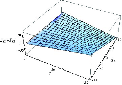
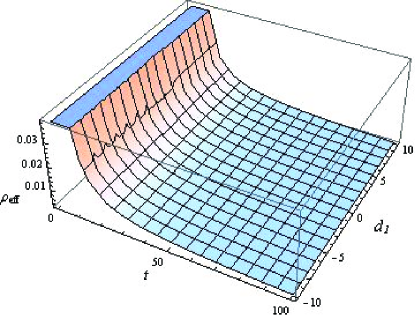
Figure 9: Energy conditions for $d_{2}=0.1$ and $d_{3}=1$.

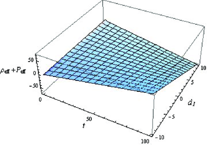
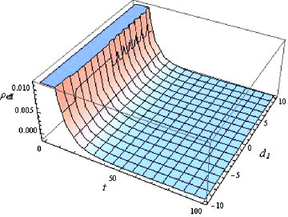
Figure 10: Energy conditions for $d_{2}=0.1$ and $d_{3}=-0.5$.

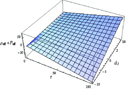
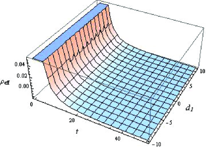
Figure 11: Energy conditions for $d_{2}=-0.1$ and $d_{3}=0.5$.

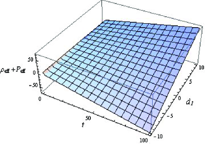
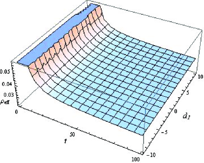
Figure 12: Energy conditions for $d_{2}=-0.1$ and $d_{3}=-1$.

The NEC and WEC depend on four parameters $t,~{}d_{1},~{}d_{2}$ and $d_{3}$. We plot these conditions against $t$ and $d_{1}$ for $n=\frac{2}{3}$ with possible signs of $d_{2}$ and $d_{3}$. The left plot of Figure 9 shows positively increasing behavior of NEC for $-10\leq d_{1}\leq 0$ with respect to time while invalid for $d_{1}>0$. The effective energy density remains positive for all values of $(t,d_{1})$ as shown in Figure 9 (right). The same behavior of both conditions are obtained for $0<d_{2}\leq 0.51$ with $d_{3}>0$ as well as for $d_{2}>0$ with $d_{3}=0$. The left plot of Figure 10 shows similar behavior of NEC for $d_{2}>0$ and $d_{3}<0$ while $\rho_{eff}$ remains positive for $0<t<23$. Similarly, for $d_{3}=-1$ and $-10$, WEC is valid for $0<t<14$ and $0<t<4.5$, respectively with $d_{2}=0.1$. The right plot of Figures 11 and 12 shows the validity of NEC for $d_{1}\geq 0$ while does not hold for negative values of $d_{1}$. The effective energy density remains positive for time interval $1\leq t\leq 10$ with $d_{3}=0.5$ as shown in Figure 11 (right panel) while for $d_{3}=1$ and $10$, the acceptable intervals are $1\leq t\leq 7$ and $1\leq t\leq 3$, respectively. This shows that the validity region of WEC decreases as the value of integration constant $d_{3}$ increases. The right plot of Figure 12 shows the positivity of $\rho_{eff}$ for $(d_{2},d_{3})<0$ which confirms the positivity of WEC with $d_{1}>0$.

5 Final Remarks

In this paper, we have presented a generalized modified theory of gravity with an arbitrary coupling between geometry and matter. The gravitational Lagrangian is obtained by adding an arbitrary function $f(\mathcal{G},T)$ in the Einstein-Hilbert action. We have formulated the corresponding field equations using least action principle and calculated the non-zero covariant divergence of $T_{\alpha\beta}$ consistent with $f(R,T)$ theory [18]. Consequently, the test particles follow non-geodesic trajectories due to the presence of extra force originated from the non-minimally coupling while they move along geodesics for pressureless fluid. We have constructed energy conditions for FRW universe model filled with dust fluid in terms of deceleration, jerk and snap $(q,j,s)$ cosmological parameters. The reconstruction technique has been applied to $f(\mathcal{G},T)$ gravity using well-known de Sitter and power-law universe models. The results are summarized as follows.

• In de Sitter reconstructed model, the energy bounds have dependence on three parameters $t,~{}c_{1}$ and $c_{2}$. We have plotted NEC and WEC against $t$ and $c_{2}$ with four possible signatures of $c_{1}$ and $c_{2}$ as shown in Figures 1-8. It is found that NEC and WEC are satisfied for $c_{1}>0$ and $c_{2}<0$ throughout the time interval while for cases $(c_{1},c_{2})>0$ and $(c_{1},c_{2})<0$, energy conditions are satisfied for small values of $c_{i}$’s in a very small time interval. It is observed that the NEC shows positively increasing behavior for all negative values of $c_{1}$ with $c_{2}>0$ while the validity ranges of WEC have dependence on $c_{1}$.

• For power-law reconstructed model, we have explored the behavior of four parameters $t,~{}d_{1},~{}d_{2}$ and $d_{3}$ with $n=\frac{2}{3}$. In this case, we have plotted energy conditions against $(t,d_{1})$ and analyzed possible behavior of remaining constants. In Figures 9-12, we have taken $-10\leq d_{1}\leq 10$ and found the valid regions where energy conditions are satisfied.

Finally, we conclude that the NEC and WEC are satisfied in both reconstructed $f(\mathcal{G},T)$ models with suitable choice of free parameters.

References

- [1] Perlmutter, S. et al.: Bull. Am. Astron. Soc. 29(1997)1351; Riess, A.G. et al.: Astron. J. 116(1998)1009; Tegmark, M. et al.: Phys. Rev. D 69(2004)103501; Spergel, D.N. et al.: Astrophys, J. Suppl. 170(2007)377.
- [2] Calcagni, G., Tsujikawa, S. and Sami, M.: Class. Quantum Grav. 22(2005)3977; De Felice, A., Hindmarsh, M. and Trodden, M.: J. Cosmol. Astropart. Phys. 08(2006)005; De Felice, A. and Tsujikawa, S.: Phys. Lett. B 675(2009)1.
- [3] Metsaev, R.R. and Tseytlin, A.A.: Nucl. Phys. B 293(1987)385; Nojiri, S., Odintsov, S.D. and Sami, M.: Phys. Rev. D 74(2006)046004; Amendola, L., Charmousis, C. and Davis, S.C.: J. Cosmol. Astropart. Phys. 10(2007)004.
- [4] Nojiri, S. and Odintsov, S.D.: Phys. Lett. B 631(2005)1.
- [5] De Felice, A. and Tsujikawa, S.: Phys. Rev. D 80(2009)063516.
- [6] Cognola, G., Elizalde, E., Nojiri, S., Odintsov, S.D. and Zerbini, S.: Phys. Rev. D 73(2006)084007; Nojiri, S. and Odintsov, S.D.: Int. J. Geom. Methods Mod. Phys. 04(2007)115.
- [7] Bertolami, O., Böhmer, C.G., Harko, T. and Lobo, F.S.N.: Phys. Rev. D 75(2007)104016; Mohseni, M.: Phys. Lett. B 682(2009)89; Harko, T. and Lobo, F.S.N.: Eur. Phys. J. C 70(2010)373.
- [8] Nojiri, S., Odintsov, S.D. and Tretyakov, P.V.: Prog. Theor. Phys. Suppl. 172(2008)81.
- [9] Carroll, S.: Spacetime and Geometry: An Introduction to General Relativity (Addison Wesley, 2004).
- [10] Schoen, R. and Yau, S.T.: Commun. Math. Phys. 79(1981)231.
- [11] Hawking, S.W. and Ellis, G.F.R.: The Large Scale Structure of Spacetime (Cambridge University Press, 1973).
- [12] Santos, J., Alcaniz, J.S., Rebouças, M.J. and Carvalho, F.C.: Phys. Rev. D 76(2007)083513; Atazadeh, K., Khaleghi, A., Sepangi, H.R. and Tavakoli, Y.: Int. J. Mod. Phys. D 18(2009)1101; García, N.M., Harko, T., Lobo, F.S.N. and Mimoso, J.P.: Phys. Rev. D 83(2011)104032; Liu, D. and Reboucas, M.J.: Phys. Rev. D 86(2012)083515.
- [13] Banijamali, A., Fazlpour, B. and Setare, M.R.: Astrophys. Space Sci. 338(2012)327.
- [14] Sharif, M. and Waheed, S. Adv. High Energy Phys. 2013(2013)253985.
- [15] Sharif, M. and Zubair, M.: J. High Energy Phys. 12(2013)079.
- [16] Landau, L.D. and Lifshitz, E.M.: The Classical Theory of Fields (Pergamon Press, 1971).
- [17] Poplawski, N.J.: arXiv:gr-qc/0608031.
- [18] Harko, T., Lobo, F.S.N., Nojiri, S. and Odintsov, S.D.: Phys. Rev. D 84(2011)024020.
- [19] Kleidis, K. and Spyrou, N.K.: Class. Quantum Grav. 17(2000)2965.
- [20] Poisson, E.: A Relativist’s Toolkit: The Mathematics of Black-Hole Mechanics (Cambridge University Press, 2004).
- [21] Dadhich, N.: arXiv:gr-qc/0511123v2; Kar, S. and Sengupta, S.: Pramana J. Phys. 69(2007)49.
- [22] Visser, M.: Class. Quantum Grav. 21(2004)2603; Gen. Relativ. Gravit. 37(2005)1541.
- [23] Sharif, M. and Zubair, M.: Gen. Relativ. Gravit. 46(2014)1723.
- [24] Capozziello, S. et al.: Phys. Rev. D 84(2011)043527; Setare, M.R. and Mohammadipour, N.: arXiv:1206.0245; Sharif, M. Rani, S. and Myrzakulov, R.: Eur. Phys. J. Plus 128(2013)123.