Aspects of Some New Versions of Pilgrim Dark Energy in DGP Braneworld

Abstract

The illustration of cosmic acceleration under two interacting dark energy models (pilgrim dark energy with Granda and Oliveros cutoff and its generalized ghost version) in DGP braneworld framework is presented. In the current scenario, the equation of state parameter, deceleration parameter, $\omega_{D}-\omega^{\prime}_{D}$ plane and statefinder diagnosis are investigated. The equation state parameter behave-like phantom era of the universe. The deceleration parameter depicts the accelerated expansion of the universe in both models. The cosmological planes like $\omega_{D}-\omega^{\prime}_{D}$ and statefinder corresponds to $\Lambda$CDM limit. To end, we remark that our results support to phenomenon of pilgrim dark energy and cosmic acceleration. Also, the results are consistent with observational data.

Keywords: DGP braneworld; PDE models; Cosmological constraints.
PACS: 95.36.+d; 98.80.-k.

1 Introduction

It has been confirmed by current observational data that the our universe undergoes accelerated expansion [1]-[6]. It is consensus that this accelerated expansion phenomenon is due to a mysterious form of force called dark energy (DE). This can be explained through the well-known parameter called equation of state (EoS) parameter $\omega_{D}$. It is suggested through WMAP data that the value of EoS parameter is bounded as $-1.11<\omega_{D}<-0.86$ [7]. This could be consistent if DE behaves like cosmological constant with $\omega_{D}=-1$ and therefore our universe seems to approach asymptotically a de Sitter universe.

In order to describe accelerated expansion phenomenon, two different approaches has been adopted. One is the proposal of various dynamical DE models such as family of chaplygin gas [8], holographic [9, 10], new agegraphic [11], polytropic gas [12], pilgrim [13]-[15] $DE$ models etc. A second approach for understanding this strange component of the universe is modifying the standard theories of gravity, namely, General Relativity (GR) or Teleparallel Theory Equivalent to GR (TEGR). Several modified theories of gravity are $f(R)$, $f(T)$ [16]-[21], $f(R,\mathcal{T})$ [22]-[23], $f(G)$ [24]-[28] (where $R$ is the curvature scalar, $T$ denotes the torsion scalar, $\mathcal{T}$ is the trace of the energy momentum tensor and $G$ is the invariant of Gauss-Bonnet defined as $G=R^{2}-4R_{\mu\nu}R^{\mu\nu}+R_{\mu\nu\lambda\sigma}R^{\mu\nu\lambda\sigma}$).

Special attention is attached to the so-called braneworld model proposed by Dvali, Gabadadze, and Porrati (DGP) [29]-[31] (for reviews, see also [32]). In a cosmological scenario, this approach leads to a late-time acceleration as a result of the gravitational leakage from a $3$-dimensional surface ($3$-brane) to a $5$-th extra dimension on Hubble distances. Hirano and Komiya [33] have generalized the modified Friedmann equation as suggested by Dvali and Turner [34] for achieving the phantom-like gap with an effective energy density with an EoS with $\omega_{D}<-1$.

The DGP model presents two branches of solutions, i.e., the self-accelerating branch ($\epsilon=+1$) and the normal ($\epsilon=-1$) one. The self accelerating branch leads to an accelerating universe without using any exotic fluid, but shows problems like ghost [35]. However, the normal branch need a DE component which is compatible with the observational data [36, 37]. The extension of these models have been studied in [38] for $f(R)$ gravity in order to obtain a self acceleration. The attempts of solutions for a DGP brane-world cosmology with a k-essence field were found in [39] showing big rip scenarios and asymptotically de Sitter phase in the future. DGP model has also been discussed by various observations without DE model (Self-accelerating DGP branch) [40]-[43] and with DE model (normal branch) [44]-[46]. However, in normal branch, the addition of dynamical DE model provides us new different structures to describe the late time acceleration with better cosmological solutions on the brane.

Holographic DE (HDE) model is the most prominent for interpreting the DE scenario and its idea comes from the unification attempt of quantum mechanics and gravity. According to t’ Hooft, quantum gravity demands three-dimensional world as a holographic image (an image whose all data can be stored on a two-dimensional projection). He stated it in the form of holographic principle, i.e., all the information relevant to a physical system inside a spatial region can be observed on its boundary instead of its volume [47]. The construction of HDE density is based on Cohen et al. [48] relation about the vacuum energy of a system with specific size whose maximum amount should not exceed the BH mass with the same size. This can be expressed as $L^{3}\rho_{\Lambda}\leq LM^{2}_{p}$, where $M^{2}_{p}=(8\pi G)^{-1}$ is the reduced Planck mass and $L$ represents the IR cutoff. We can get HDE density from the above inequality as

$$\rho_{\Lambda}=3c^{2}M^{2}_{p}L^{-2},$$ (1)

here $c$ is the dimensionless HDE constant parameter. The interesting feature of HDE density is that it provides a relation between ultraviolet (bound of vacuum energy density) and IR (size of the universe) cutoffs. However, a controversy about the selection of IR cutoff of HDE has been raised since its birth. As a result, different people have suggested different expressions.

In the present paper, we check the role of some new models of pilgrim DE (PDE) (pilgrim dark energy with Granda and Oliveros (GO) cutoff and its generalized ghost version) in DGP Braneworld. We develop different cosmological parameters and planes. This paper is outlined as follows: In section 2, we provide the basics of the DGP braneworld model and explain the PDE models. Sections 3 and 4 are devoted for cosmological parameters and cosmological planes for new models of PDE. In the last section, we conclude our results.

2 DGP Braneworld Model and Pilgrim Dark Energy

Now we define the cosmological evolution on the brane by Friedmann equation as [32]

$$H^{2}+\frac{k}{a^{2}}=\bigg{(}\sqrt{\frac{\rho}{3}+\frac{1}{4r_{c}^{2}}}+\frac{\epsilon}{2r_{c}}\bigg{)}^{2},$$ (2)

where $\rho=\rho_{M}+\rho_{D}$ is the total cosmic fluid energy density on the brane ($\rho_{M}$ is the CDM density while $\rho_{D}$ is the PDE density). Also, $r_{c}$ is the crossover length given by [49]

$$r_{c}=\frac{M_{pl}^{2}}{2M_{5}^{3}}=\frac{G_{5}}{2G_{4}},$$ (3)

$r_{c}$ is defined as a distance scale reflecting the competition between $4D$ and $5D$ effects of gravity. Below the length $r_{c}$, gravity appears $4$-dim and above the length $r_{c}$, gravity can leak into the extra dimension. For the spatially flat DGP Braneworld $(k=0)$, the Friedmann equation (3) reduces to

$$H^{2}-\frac{\epsilon}{r_{c}}H=\frac{1}{3}(\rho_{M}+\rho_{D}).$$ (4)

Since, we are taking the interaction between DE and CDM, hence the conservation equations turn out to be

$$\dot{\rho}_{M}+3H\rho_{M}=Q\quad\dot{\rho}_{D}+3H(\rho_{D}+p_{D})=-Q,$$ (5)

here $Q$ describes the interaction between PDE and CDM. We choose $Q=3b^{2}H\rho_{m}$ as an interaction term with $b^{2}$ being a coupling constant. This interaction term is used for transferring the energy through different cosmological constraints. Its positive sign indicates that DE decays into CDM and negative sign shows that CDM decays into DE. Here, we take $Q$ as positive because it is more favorable with observational data. Hence, with this interaction form, Eq. (5) provides

$$\rho_{M}=\rho_{M_{0}}a^{3(b^{2}-1)},$$ (6)

here $\rho_{M_{0}}$ is the integration constant.

Further, we illustrate the discussion about under consideration model called PDE. Cohen et al. [47] relation leads to the bound of energy density from the idea of formation of BH in quantum gravity. However, it is suggested that formation of BH can be avoided through appropriate repulsive force which resists the matter collapse phenomenon. The phantom-like DE possesses the appropriate repulsive force (in spite of other phases of DE like vacuum or quintessence DE). By keeping in mind this phenomenon, Wei [13] has suggested the DE model called PDE on the speculation that phantom DE possesses the large negative pressure as compared to the quintessence DE which helps in violating the null energy condition and possibly prevent the formation of BH. In the past, many applications of phantom DE exist in the literature. It is also playing an important role in the reduction of mass due to its accretion process onto BH. Many works have been done in this support through a family of chaplygin gas [50]-[53]. For instance, phantom DE is also play an important role in the wormhole physics where the event horizon can be avoided due to its presence [54]-[57].

It was also argued that BH area reduces up to $50$ percent through phantom scalar field accretion onto it [58]. According to Sun [59], mass of BH tends to zero when the universe approaches to big rip singularity. It was also suggested that BHs might not be exist in the universe in the presence of quintessence-like DE which violates only strong energy condition [60]. However, these works do not correspond to reality because quintessence DE does not contain enough resistive force to in order to avoid the formation of BH. Also, Saridakis et al. [61]-[70] have obtained the phantom crossing, quintom as well as phantom-like nature of the universe in different frameworks and found interesting results in this respect.

The above discussion is motivated to Wei [13] in developing the $PDE$ model. He analyzed this model with Hubble horizon through different theoretical as well as observational aspects. The energy density for PDE model with hubble horizon is defined as

$$\rho_{D}=3c^{2}L^{-u}.$$ (7)

where $u$ is the PDE parameter, $m_{pl}=1$ and $L$ is known as IR cutoff. The proposal of PDE model by Wei [13] is based on two properties. The first property of PDE is

$$\rho_{D}\gtrsim m_{p}^{2}L^{-2}.$$ (8)

From Eqs.(7) and (8), we have $L^{2-u}\gtrsim m_{p}^{u-2}=l_{p}^{2-u}$, where $l_{p}$ is the reduced Plank length. Since $L>l_{p}$, one requires

$$u\leq 2.$$ (9)

The second requirement for PDE is that it gives phantom-like behavior [13]

$$\omega_{D}<-1$$ (10)

It is stated [13] that a particular cutoff $L$ has to choose to obtain the EoS for PDE. For instance, radius of Hubble horizon $L=H^{-1}$, event horizon $L=R_{E}=a\int_{t}^{\infty}\frac{dt}{a}$, the form $L=(H^{2}+\dot{H})^{-\frac{1}{2}}$ represented the Ricci length, the GO length $(\alpha H^{2}+\beta\dot{H})^{-\frac{1}{2}}$, etc.

Recently, we have investigated this model by taking different IR cutoffs in flat as well as non-flat FRW universe with different cosmological parameters as well as cosmological planes [14, 15]. This model has also been investigated in different modify gravity theories [71]-[73]. In the next two sections, we will discuss the cosmological parameters of PDE with GO cutoff and ghost version of PDE.

3 Pilgrim Dark Energy with Granda and Oliveros Cutoff

Granda and Oliveros [74] deveoped IR cutoff (involving Hubble parameter and its derivative) of HDE parameterized by two dimensionless constants called new HDE (NHDE). They suggested that this model can be an effective candidate in solving the cosmic coincidence problem. Yu et al. [75] analyzed the behavior of interacting NHDE with CDM and found that this model inherits the features of already presented HDE models. Also, constraints on different cosmological parameters are established for this model by using the data of different observational schemes and Markov chain Monte Carlo method [76]. The GO cutoff can be defined as follows [77]

$$\rho_{D}=3(\alpha H^{2}+\beta\dot{H}).$$ (11)

Where $\alpha$ and $\beta$ are the positive constants. With GO cutoff, the PDE model turns out to be

$$\rho_{D}=3(\alpha{H^{2}}+\beta{\dot{H}})^{u/2}.$$ (12)

By taking the time derivative of Eq.(4) and then by using the Eq.(12), we get

$$\frac{\dot{H}}{H^{2}}=\frac{1}{H^{2}\beta}\bigg{(}H^{2}(1-2\epsilon\sqrt{\Omega_{r_{c}}})-\frac{1}{3}\rho_{m_{{}_{0}}}a^{-3(1-b^{2})}\bigg{)}^{2/u}-\frac{\alpha}{\beta}.$$ (13)

where $\Omega_{r_{c}}=\frac{1}{4H^{2}r^{2}_{c}}$. By solving the Eqs.(5) and (12), we obtain the EoS parameter

$$\omega_{D} = -1-\frac{2(1-\epsilon\sqrt{\Omega_{r_{c}}})}{3H^{2}}\big{(}(1-2\epsilon\sqrt{\Omega_{r_{c}}})-\frac{\rho_{m_{{}_{0}}}a^{-3(1-b^{2})}}{3H^{2}}\big{)}^{-1}$$ (14)

$$\times \frac{1}{\beta}\bigg{(}\big{(}H^{2}(1-2\epsilon\sqrt{\Omega_{r_{c}}})-\frac{1}{3}\rho_{m_{{}_{0}}}a^{-3(1-b^{2})}\big{)}^{2/u}-\alpha H^{2}\bigg{)}$$

$$+ \frac{(2b^{2}+1)\rho_{m_{{}_{0}}}a^{-3(1-b^{2})}}{3H^{2}}\bigg{(}(1-2\epsilon\sqrt{\Omega_{r_{c}}})-\frac{\rho_{m_{{}_{0}}}a^{-3(1-b^{2})}}{3H^{2}}\bigg{)}^{-1}.$$

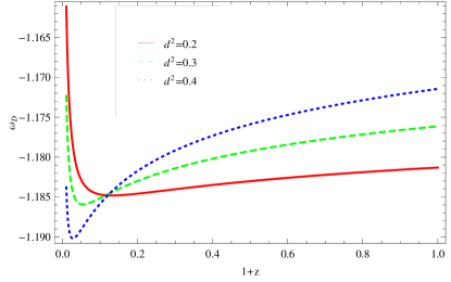
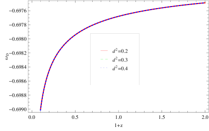
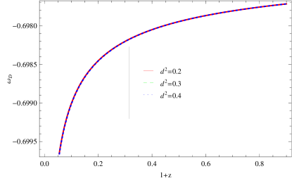
Figure 1: Plots of $\omega_{D}$ versus $1+z$ for new PDE model in DGP with u=1 (upper left panel), $u=-1$ (upper right panel), $u=-2$ (lower panel), respectively.

The deceleration parameter can be defined as follows:

$$q=-1-\frac{\dot{H}}{H^{2}}.$$ (15)

The deceleration parameter can also be obtain by using the Eqs. (13) and (15) as

$$q=-1-\frac{1}{\beta H^{2}}\bigg{(}H^{2}(1-2\epsilon\sqrt{\Omega_{r_{c}}})-\frac{1}{3}\rho_{m_{{}_{0}}}a^{-3(1-b^{2})}\bigg{)}^{2/u}+\frac{\alpha}{\beta}.$$ (16)

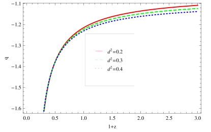
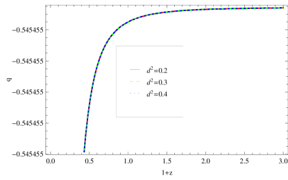
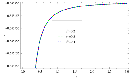
Figure 2: Plots of $q$ versus $1+z$ for new PDE model in DGP with u=1 (upper left panel), $u=-1$ (upper right panel), $u=-2$ (lower panel), respectively.

Here, we find the regions on the $\omega_{\vartheta}-\omega^{\prime}_{\vartheta}$ plane ($\omega^{\prime}_{\vartheta}$ represents the evolution of $\omega_{\vartheta}$) as defined by Caldwell and Linder [78] for models under consideration. The models can be categorized in two different classes as thawing and freezing regions on the $\omega_{\vartheta}-\omega^{\prime}_{\vartheta}$ plane. The thawing models describe the region $\omega^{\prime}_{\vartheta}>0$ when $\omega_{\vartheta}<0$ and freezing models represent the region $\omega^{\prime}_{\vartheta}<0$ when $\omega_{\vartheta}<0$. Initially, this phenomenon was applied for analyzing the behavior of quintessence model and found that the corresponding area occupied on the $\omega_{\vartheta}-\omega^{\prime}_{\vartheta}$ plane describes the thawing and freezing regions.

The differentiation of EoS parameter Eq. (14) w.r.t. $x=\ln a$ leads to

$$\omega^{\prime}_{D} = -\frac{1}{3}\bigg{(}H^{2}(1-2\epsilon\sqrt{\Omega_{r_{c}}})-\frac{1}{3}\rho_{m_{{}_{0}}}a^{-3(1-b^{2})}\bigg{)}^{-1}\bigg{(}\frac{2}{H}(1-\epsilon\sqrt{\Omega_{r_{c}}})$$ (17)

$$\times \bigg{(}\frac{2}{u\beta}\big{(}H^{2}(1-2\epsilon\sqrt{\Omega_{r_{c}}})-\frac{1}{3}\rho_{m_{{}_{0}}}a^{-3(1-b^{2})}\big{)}^{\frac{2}{u}-1}\big{(}2(1-\epsilon\sqrt{\Omega_{r_{c}}})$$

$$\times \big{(}\frac{1}{\beta}\big{(}H^{2}(1-2\epsilon\sqrt{\Omega_{r_{c}}})-\frac{1}{3}\rho_{m_{{}_{0}}}a^{-3(1-b^{2})}\big{)}^{2/u}-\frac{\alpha}{\beta}H^{2}\big{)}+(1-b^{2})$$

$$\times \rho_{m_{{}_{0}}}a^{-3(1-b^{2})}H\big{)}-\frac{2\alpha}{\beta}H\big{(}\frac{1}{\beta}\big{(}H^{2}(1-2\epsilon\sqrt{\Omega_{r_{c}}})-\frac{1}{3}\rho_{m_{{}_{0}}}a^{-3(1-b^{2})}\big{)}^{2/u}$$

$$- \frac{\alpha}{\beta}H^{2}\big{)}\bigg{)}+2\epsilon\sqrt{\Omega_{r_{c}}}\big{(}\frac{1}{\beta H^{2}}\big{(}H^{2}(1-2\epsilon\sqrt{\Omega_{r_{c}}})-\frac{1}{3}\rho_{m_{{}_{0}}}a^{-3(1-b^{2})}\big{)}^{2/u}$$

$$- \frac{\alpha}{\beta}\big{)}-3(1-b^{2})^{2}\rho_{m_{{}_{0}}}a^{-3(1-b^{2})}-9b^{2}(1-b^{2})\rho_{m_{{}_{0}}}a^{-3(1-b^{2})}\bigg{)}+\frac{1}{3}$$

$$\times \bigg{(}H^{2}(1-2\epsilon\sqrt{\Omega_{r_{c}}})-\frac{1}{3}\rho_{m_{{}_{0}}}a^{-3(1-b^{2})}\bigg{)}^{-2}\bigg{(}2(1-\epsilon\sqrt{\Omega_{r_{c}}})\big{(}\frac{1}{\beta}\big{(}H^{2}$$

$$\times (1-2\epsilon\sqrt{\Omega_{r_{c}}})-\frac{1}{3}\rho_{m_{{}_{0}}}a^{-3(1-b^{2})}\big{)}^{2/u}-\frac{\alpha}{\beta}H^{2}\big{)}+(1-b^{2})\rho_{m_{{}_{0}}}$$

$$\times a^{-3(1-b^{2})}+3b^{2}\rho_{m_{{}_{0}}}a^{-3(1-b^{2})}\bigg{)}\bigg{(}2(1-\epsilon\sqrt{\Omega_{r_{c}}})\big{(}\frac{1}{\beta}\big{(}H^{2}(1-2\epsilon$$

$$\times \sqrt{\Omega_{r_{c}}})-\frac{1}{3}\rho_{m_{{}_{0}}}a^{-3(1-b^{2})}\big{)}^{2/u}-\frac{\alpha}{\beta}H^{2}\big{)}+(1-b^{2})\rho_{m_{{}_{0}}}a^{-3(1-b^{2})}\bigg{)}.$$

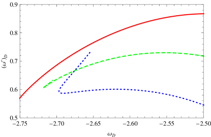
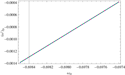
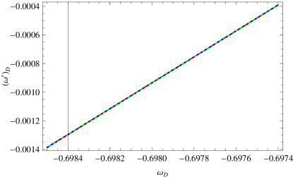
Figure 3: Plots of $\omega_{D}-\omega^{\prime}_{D}$ for new PDE model in DGP with u=1 (upper left panel), $u=-1$ (upper right panel), $u=-2$ (lower panel), respectively.

The Hubble parameter $H$ and the deceleration parameter $q$ cannot discriminate among various DE models. For this purpose Sahni et al. [79] and Alam et al. [80] proposed a new geometrical diagnostic pair for DE and it is constructed from the scale factor $a(t)$ and its derivatives up to third order. The statefinder pair $(r,s)$ is defined as

$$r=\frac{\dddot{a}}{aH^{3}},s=\frac{r-1}{3(q-1/2)}.$$ (18)

The state-finder parameter $r$ can be expressed as

$$r=1+3\frac{\dot{H}}{H^{2}}+\frac{\ddot{H}}{H^{3}}.$$ (19)

By using the relations (18), (19) and (13), we obtain the state-finder parameters $(r,s)$ as

$$r = 1+\bigg{(}\frac{1}{\beta H^{2}}\big{(}H^{2}(1-2\epsilon\sqrt{\Omega_{r_{c}}})-\frac{1}{3}\rho_{m_{{}_{0}}}a^{-3(1-b^{2})}\big{)}^{2/u}-\frac{\alpha}{\beta}\bigg{)}\bigg{(}3$$ (20)

$$+ \frac{4}{\beta u}(1-\epsilon\sqrt{\Omega_{r_{c}}})(H^{2}(1-2\epsilon\sqrt{\Omega_{r_{c}}})-\frac{\rho_{m_{{}_{0}}}a^{-3(1-b^{2})}}{3})^{\frac{2}{u}-1}-2\frac{\alpha}{\beta}\bigg{)}$$

$$+ \frac{2(1-b^{2})}{u\beta H^{2}}\rho_{m_{{}_{0}}}a^{-3(1-b^{2})}\big{(}H^{2}(1-2\epsilon\sqrt{\Omega_{r_{c}}})-\frac{1}{3}\rho_{m_{{}_{0}}}a^{-3(1-b^{2})}\big{)}^{\frac{2}{u}-1}.$$

$$s = \frac{1}{3}\bigg{(}\frac{-3}{2}-\frac{1}{\beta H^{2}}(H^{2}(1-2\epsilon\sqrt{\Omega_{r_{c}}}))^{2/u}+\frac{\alpha}{\beta}\bigg{)}^{-1}\bigg{(}\big{(}\frac{1}{\beta H^{2}}(H^{2}$$ (21)

$$\times (1-2\epsilon\sqrt{\Omega_{r_{c}}})-\frac{1}{3}\rho_{m_{{}_{0}}}a^{-3(1-b^{2})})^{2/u}+\frac{\alpha}{\beta}\big{)}\big{(}3+\frac{4}{\beta u}(1-\epsilon\sqrt{\Omega_{r_{c}}})$$

$$\times (H^{2}(1-2\epsilon\sqrt{\Omega_{r_{c}}})-\frac{\rho_{m_{{}_{0}}}a^{-3(1-b^{2})}}{3})^{\frac{2}{u}-1}-2\frac{\alpha}{\beta}\big{)}+\frac{2(1-b^{2})}{u\beta H^{2}}$$

$$\times \rho_{m_{{}_{0}}}a^{-3(1-b^{2})}\big{(}H^{2}(1-2\epsilon\sqrt{\Omega_{r_{c}}})-\frac{1}{3}\rho_{m_{{}_{0}}}a^{-3(1-b^{2})}\big{)}^{\frac{2}{u}-1}\bigg{)}.$$

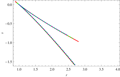
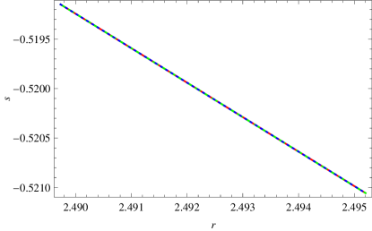
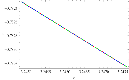
Figure 4: Plots of $r-s$ for new PDE model in DGP with u=1 (upper left panel), $u=-1$ (upper right panel), $u=-2$ (lower panel), respectively.

The behavior of EoS parameter in terms of redshift parameter (by utilizing $a=(1+z)^{-1}$) is displayed in Figure 1 for $u=1,-1,-2$ (since there is property of PDE for attaining useful results, we should choose $u\leq 2$, that is why we have chosen $u=1,-1,-2$). The EoS parameter shows the phantom-like behavior for $u=1$ (left panel of Figure 1) while exhibits quintessence-like behavior for $u=-1,-2$ (right and lower panels of Figure 1). However, the deceleration parameter remains less than $0$ i.e., $q<0$ for all values of $u$ (Figure 2). Hence, the deceleration parameter exhibits the accelerated expansion of the universe. We also developed $\omega_{D}-\omega^{\prime}_{D}$ plane for $u=1,-1,-2$ as shown in Figure 3. It can be seen that this plane corresponding to for $u=1$ lies in the thawing region, while lie in the freezing region for $u=-1,-2$. The $r-s$ planes for $u=1,-1,-2$ are shown in Figure 4 which behave like chaplygin gas model. However, the $\Lambda$CDM limit is also achieved for $u=-1$ case.

4 Generalized Ghost Pilgrim Dark Energy

The generalized ghost version of PDE can be defined as [81]

$$\rho_{D}=(\alpha H+\beta H^{2})^{u}.$$ (22)

Equations (4) and (22) gives the Hubble parameter for this model as follows

$$\frac{\dot{H}}{H^{2}}=-\frac{1}{H^{2}}\bigg{(}\frac{(1-b^{2})\rho_{m_{0}}a^{-3(1-b^{2})}}{2-2\epsilon\sqrt{\Omega_{r}}-\frac{u}{3H}(\alpha{H}+\beta{H^{2}})^{u-1}(\alpha+2\beta{H})}\bigg{)}.$$ (23)

This leads to deceleration parameter as follows

$$q=-1+\frac{1}{H^{2}}\bigg{(}\frac{(1-b^{2})\rho_{m_{0}}a^{-3(1-b^{2})}}{2-2\epsilon\sqrt{\Omega_{r}}-\frac{u}{3H}(\alpha{H}+\beta{H^{2}})^{u-1}(\alpha+2\beta{H})}\bigg{)}.$$ (24)

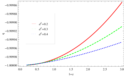
Figure 5: Plots of $q$ versus $1+z$ for GGPDE model in DGP with u=1 (upper left panel), $u=-1$ (upper right panel), $u=-2$ (lower panel), respectively.

However, the EoS parameter can be obtained by using Eqs. (5) and (24)

$$\omega_{D} = -1-\frac{b^{2}\rho_{m_{0}}a^{-3(1-b^{2})}}{(\alpha H+\beta H^{2})^{u}}-\frac{u}{3H}\big{(}\frac{\alpha+2\beta H}{\alpha H+\beta H^{2}}\big{)}\bigg{(}-\frac{1}{H^{2}}$$ (25)

$$\times \big{(}\frac{(1-b^{2})\rho_{m_{0}}a^{-3(1-b^{2})}}{2-2\epsilon\sqrt{\Omega_{r}}-\frac{u}{3H}(\alpha{H}+\beta{H^{2}})^{u-1}(\alpha+2\beta{H})}\big{)}\bigg{)}.$$

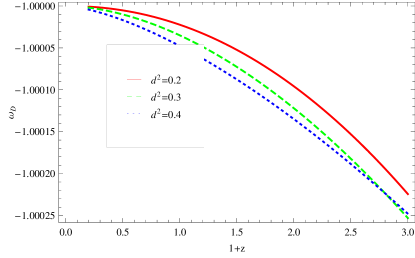
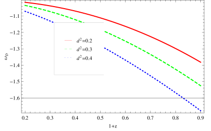
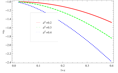
Figure 6: Plots of $\omega_{\vartheta}$ versus $1+z$ for GGPDE model in DGP with u=1 (upper left panel), $u=-1$ (upper right panel), $u=-2$ (lower panel), respectively.

The derivative of Eq.(24) w.r.t. $x$ leads to

$${\omega_{D}}^{\prime} = 3b^{2}(1-b^{2})\rho_{m_{0}}a^{-3(1-b^{2})}\big{(}\alpha H+\beta H^{2}\big{)}^{-u}+ub^{2}\rho_{m_{0}}a^{-3(1-b^{2})}$$ (26)

$$\times H^{-1}\big{(}\alpha H+\beta H^{2}\big{)}^{-u-1}(\alpha+2\beta H)\bigg{(}-(1-b^{2})\rho_{m_{0}}a^{-3(1-b^{2})}$$

$$\times \big{(}2-2\epsilon\sqrt{\Omega_{r}}-\frac{u}{3H}(\alpha{H}+\beta{H^{2}})^{u-1}(\alpha+2\beta H)\big{)}^{-1}\bigg{)}-\frac{u}{3H^{2}}$$

$$\times (\frac{\alpha+2\beta H}{\alpha H+\beta H^{2}})\bigg{(}\bigg{(}3(1-b^{2})^{2}\rho_{m_{0}}a^{-3(1-b^{2})}H\big{(}2-2\epsilon\sqrt{\Omega_{r}}-\frac{u}{3H}$$

$$\times (\alpha{H}+\beta{H^{2}})^{u-1}(\alpha+2\beta H)\big{)}^{-1}\bigg{)}+\bigg{(}(1-b^{2})\rho_{m_{0}}a^{-3(1-b^{2})}$$

$$\times \big{(}2-2\epsilon\sqrt{\Omega_{r}}-\frac{u}{3H}(\alpha{H}+\beta{H^{2}})^{u-1}(\alpha+2\beta H)\big{)}^{-2}\bigg{)}H^{-1}$$

$$\times \big{(}-(1-b^{2})\rho_{m_{0}}a^{-3(1-b^{2})}\big{(}2-2\epsilon\sqrt{\Omega_{r}}-\frac{u}{3H}(\alpha{H}+\beta{H^{2}})^{u-1}$$

$$\times (\alpha+2\beta H)\big{)}^{-1}\big{)}\bigg{(}2\epsilon\sqrt{\Omega_{r}}-\frac{u(u-1)}{3}(\alpha{H}+\beta{H^{2}})^{u-2}(\alpha$$

$$+ 2\beta H)^{2}+\frac{u\alpha}{3H}(\alpha{H}+\beta{H^{2}})^{u-1}\bigg{)}\bigg{)}+\frac{u}{3H^{2}}(2\alpha^{2}+4H^{2}\beta^{2}$$

$$+ 5H\alpha\beta)(\alpha H+\beta H^{2})^{-2}\bigg{(}-(1-b^{2})\rho_{m_{0}}a^{-3(1-b^{2})}\big{(}2-2$$

$$\times \epsilon\sqrt{\Omega_{r}}-\frac{u}{3H}(\alpha{H}+\beta{H^{2}})^{u-1}(\alpha+2\beta H)\big{)}^{-1}\bigg{)}^{2}.$$

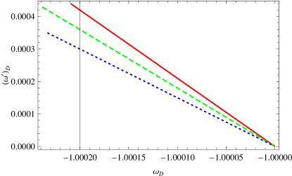
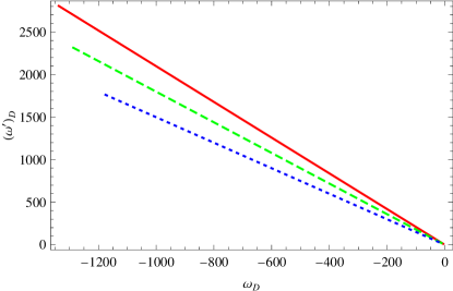
Figure 7: Plots of $\omega_{D}-\omega^{\prime}_{D}$ GGPDE model in DGP with u=1 (upper left panel), $u=-1$ (upper right panel), $u=-2$ (lower panel), respectively.

After solving the Eqs.(18), (19) and (22), we can obtain the statefinder parameter as

$$r = 1-\bigg{(}\frac{1}{H^{2}}\big{(}\frac{(1-b^{2})\rho_{m_{0}}a^{-3(1-b^{2})}}{2-2\epsilon\sqrt{\Omega_{r}}-\frac{u}{3H}(\alpha{H}+\beta{H^{2}})^{u-1}(\alpha+2\beta{H})}\big{)}\bigg{)}$$ (27)

$$\times \bigg{(}3+(1-b^{2})\rho_{m_{0}}a^{-3(1-b^{2})}\big{(}2-2\epsilon\sqrt{\Omega_{r}}-\frac{u}{3H}(\alpha{H}+\beta{H^{2}})^{u-1}$$

$$\times (\alpha+2\beta{H})\big{)}^{-2}\big{(}2-2\epsilon\sqrt{\Omega_{r}}-\frac{u(u-1)}{3H}(\alpha{H}+\beta{H^{2}})^{u-2}$$

$$\times (\alpha+2\beta{H})^{2}+\frac{u\alpha}{3H}(\alpha H+\beta H^{2})^{u-1}\big{)}\bigg{)}+\frac{3}{H^{2}}\rho_{m_{0}}a^{-3(1-b^{2})}$$

$$\times (1-b^{2})\bigg{(}2-2\epsilon\sqrt{\Omega_{r}}-\frac{u}{3H}(\alpha{H}+\beta{H^{2}})^{u-1}(\alpha+2\beta{H})\bigg{)}.$$

$$s = \frac{1}{3}\bigg{(}-\frac{3}{2}+\frac{1}{H^{2}}\big{(}\frac{(1-b^{2})\rho_{m_{0}}a^{-3(1-b^{2})}}{2-2\epsilon\sqrt{\Omega_{r}}-\frac{u}{3H}(\alpha{H}+\beta{H^{2}})^{u-1}(\alpha+2\beta{H})}\big{)}\bigg{)}^{-1}$$ (28)

$$\times \bigg{(}\frac{1}{H^{2}}\big{(}\frac{(1-b^{2})\rho_{m_{0}}a^{-3(1-b^{2})}}{2-2\epsilon\sqrt{\Omega_{r}}-\frac{u}{3H}(\alpha{H}+\beta{H^{2}})^{u-1}(\alpha+2\beta{H})}\big{)}\big{(}3+(1-b^{2})$$

$$\times \rho_{m_{0}}a^{-3(1-b^{2})}\big{(}2-2\epsilon\sqrt{\Omega_{r}}-\frac{u}{3H}(\alpha{H}+\beta{H^{2}})^{u-1}(\alpha+2\beta{H})\big{)}^{-2}$$

$$\times \big{(}2-2\epsilon\sqrt{\Omega_{r}}-\frac{u(u-1)}{3H}(\alpha{H}+\beta{H^{2}})^{u-2}(\alpha+2\beta{H})^{2}+\frac{u\alpha}{3H}$$

$$\times (\alpha H+\beta H^{2})^{u-1}\big{)}\big{)}+\frac{3}{H^{2}}(1-b^{2})\rho_{m_{0}}a^{-3(1-b^{2})}\big{(}2-2\epsilon\sqrt{\Omega_{r}}$$

$$- -\frac{u}{3H}(\alpha{H}+\beta{H^{2}})^{u-1}(\alpha+2\beta{H})\big{)}\bigg{)}.$$

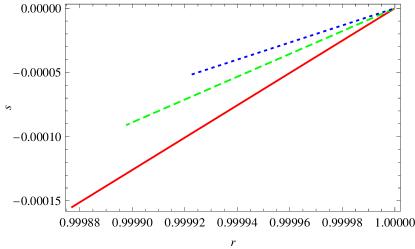
Figure 8: Plots of $r-s$ for GGPDE model in DGP with u=1 (upper left panel), $u=-1$ (upper right panel), $u=-2$ (lower panel), respectively.

The deceleration parameter indicates the cosmic acceleration because it lies within the range ($-1,0$) for all values of $u$ (Figure 5). For this case, EoS parameter represents the phantom-like behavior of the universe for all values of $u=1,-1,-2$ (Figure 6). We also developed $\omega_{D}-\omega^{\prime}_{D}$ plane for this case for $u=1,-1,-2$ as shown in Figure 7. It can be seen that this plane corresponding to thawing region as well as to $\Lambda$CDM limit for all values of $u$. The $r-s$ planes for $u=1,-1,-2$ also approaches to $\Lambda$CDM limit for all values of $u$ (Figure 8).

5 Conclusion

In the present paper, we have investigated the cosmological implications by assuming two interacting DE models such as PDE with GO cutoff and GGPDE. We have explored various cosmological parameters as well as planes for these two DE models. The results are illustrated as follows: The EoS parameter have depicted the phantom-like behavior for $u=1$ (left panel of Figure 1) while exhibits quintessence-like behavior for $u=-1,-2$ (right and lower panels of Figure 1) for PDE with GO cutoff. However, the phantom-like behavior of the universe for all values of $u=1,-1,-2$ (Figure 6) for GGPDE. The trajectories of deceleration parameter have also indicated the accelerated expansion of the universe in both DE models (Figures 2 and 5). The $\omega_{D}-\omega^{\prime}_{D}$ plane corresponding to $u=1$ lies in the thawing region, while lie in the freezing region for $u=-1,-2$ for PDE with GO cutoff (Figure 3). For GGPDE, it can be seen that this plane corresponding to thawing region as well as to $\Lambda$CDM limit for all values of $u$ (Figure 7). For PDE with GO cutoff, the $r-s$ planes for $u=1,-1,-2$ have shown in Figure 4 which behave like chaplygin gas model. However, the $\Lambda$CDM limit is also achieved for $u=-1$ case. On the other hand, the $r-s$ planes for $u=1,-1,-2$ also approaches to $\Lambda$CDM limit for all values of $u$. Finally, it is remarked that all the cosmological parameters in the present scenario shows compatibility with the current well-known observational data [82]-[84].

References

- [1] A. G. Riess et al., Astron. J. 116, 1009 (1998)
- [2] S. Perlmutter et al., Astrophys. J. 517, 565 (1999)
- [3] P. de Bernardis et al., Nature 404, 955 (2000)
- [4] S. Hanany et al., Astrophys. J. 545, L5 (2000).
- [5] P. J. E. Peebles and B. Ratra, Rev. Mod. Phys. 75, 559 (2003)
- [6] T. Padmanabhan, Phys. Repts. 380, 235 (2003)
- [7] E. Komatsu et al (WMAP Collaboration) Astrophys. J. Suppl. 180, 330-376, (2009).
- [8] Kamenshchik, A.Y., Moschella, U. and Pasquier, V.: Phys. Lett. B 511(2001)265.
- [9] Hsu, S.D.H.: Phys. Lett. B 594(2004)13.
- [10] Li, M.: Phys. Lett. B 603(2004)1.
- [11] Cai, R.G.: Phys. Lett. B 660(2008)113.
- [12] Karami, K., Ghaffari, S. and Fehri, J.: Eur. Phys. J. C 64(2009)85.
- [13] Wei, H.: Class. Quantum Grav. 29, 175008 (2012).
- [14] Sharif, M. and Jawad, A.: Eur. Phys. J. C 73, 2382 (2013).
- [15] Sharif, M. and Jawad, A.: Eur. Phys. J. C 73, 2600 (2013).
- [16] J. Amorós, J. de Haro and S. D. Odintsov, Physical Review D 87, 104037 (2013).
- [17] E. V. Linder, Phys.Rev. D 81, 127301 (2010) [Erratum-ibid. D 82, 109902 (2010)]
- [18] M. Jamil, D. Momeni and R. Myrzakulov, Eur. Phys. J. C 72 (2012) 2267.
- [19] R. Myrzakulov, Entropy 14 (2012) 1627.
- [20] I.G.Salako, M.E.Rodrigues, A.V.Kpadonou, M. J.S.Houndjo and J.Tossa: JCAP 060, 1475-7516 (2013).
- [21] M. E. Rodrigues, I. G. Salako, M. J. S. Houndjo, J. Tossa Int. J. Mod. Phys. D 23, 1450004 (2014).
- [22] E. H. Baffou, A. V. Kpadonou, M. E. Rodrigues, M. J. S. Houndjo, and J. Tossa Astrophys.Space Sci 355, 2197 (2014).
- [23] M. J. S. Houndjo, Int. J. Mod. Phys. D. 21, 1250003 (2012).
- [24] S. ’i. Nojiri and S. D. Odintsov, Phys. Lett. B 631, 1 (2005). S. Nojiri, S. D. Odintsov, A. Toporensky, P. Tretyakov, arXiv:0912.2488.
- [25] K. Bamba, S. D. Odintsov, L. Sebastiani, S. Zerbini: arXiv:0911.4390.
- [26] K. Bamba, C.-Q. Geng, S. Nojiri, S. D. Odintsov: arXiv:0909.4397.
- [27] M.E. Rodrigues, M.J.S. Houndjo, D. Momeni, R. Myrzakulov: arXiv:1212.4488.
- [28] M. J. S. Houndjo, M. E. Rodrigues, D. Momeni, R. Myrzakulov, arXiv:1301.4642.
- [29] G. R. Dvali, G. Gabadadze, and M.Porrati, Phys. Lett. B 485 (2000) 208.
- [30] C. Deffayet, Phys. Lett. B 502 (2001) 199.
- [31] C. Deffayet, G.R. Dvali, G. Gabadadze, Phys. Rev. D 65 (2002) 044023.
- [32] K. Koyama Gen. Rel. Grav. 40 (2008) 421.
- [33] K. Hirano and Z. Komiya Gen. Rel. Grav. 42 (2010) 2751, [arXiv:0912.4950 [astroph.CO]].
- [34] G. Dvali and M.S. Turner arXiv:astro-ph/0301510.
- [35] K. Koyama, Class. Quant. Grav. 24, R231 (2007) [arXiv:0709.2399 [hep-th]].
- [36] A. Lue and G. D. Starkman, Phys. Rev. D 70, 101501 (2004) [arXiv:astro-ph/0408246].
- [37] R. Lazkoz, R. Maartens and E. Majerotto, Phys. Rev. D 74, 083510 (2006) [arXiv:astro-ph/0605701].
- [38] M. Bouhmadi-Lopez, JCAP 0911:011 (2009).
- [39] M. Bouhmadi-Lopez and L. Chimento, Phys.Rev.D82:103506 (2010).
- [40] Luty, M.A. et al.: JHEEP 09(2003)029.
- [41] Goobar, A. et al.: Phys. Lett. B 642(2006)432; Majerotto, E. et al.: Phys. Rev. D 74(2006)023004.
- [42] Wang, Y. et al.: Phys. Rev. D 82(2010)043503.
- [43] Dvali, J.: New. J. Phys. 8(2006)326; Koyoma, K.: Class. Quant. Grav. 24(2007)231-253.
- [44] Aguilera, Y.: Eur. Phys. J. C 74(2014)3172.
- [45] Ghaffari, S., Dehghani, H. and Sheykhi, A.: Phys. Rev. D 89(2014)123009.
- [46] Ghaffari, S., Sheykhi, A. and Dehghani, H.: Phys. Rev. D 91(2015)023007.
- [47] t’ Hooft, G.: Dimensional Reduction in Quantum Gravity, gr-qc/9310026; Susskind, L.: J. Math. Phys. 36(1995)6377.
- [48] Cohen, A., Kaplan, D. and Nelson, A.: Phys. Rev. Lett. 82(1999)4971.
- [49] Akama, A. Lect. Notes Phys.: 176(1982)0001113.
- [50] Jawad, A. and Shahzad, M. U..: Eur. Phys. J. C 76(2016)123.
- [51] Sharif, M. and Jawad, A.: Int. J. Mod. Phys. D 22, 1350014 (2013).
- [52] Jamil, M.: Eur. Phys. J. C 62(2009)325.
- [53] Bhadra, J. and Debnath, U.: Eur. Phys. J. C 72(2012)1912.
- [54] Sharif, M. and Jawad, A.: Eur. Phys. J. Plus 129, 15 (2014).
- [55] Lobo, F.S.N.: Phys. Rev. D 71(2005)124022.
- [56] Lobo, F.S.N.: Phys. Rev. D 71(2005)084011.
- [57] Sushkov, S.: Phys. Rev. D 71(2005)043520.
- [58] Gonzalez, J.A. and Guzman, F.S.: Phys. Rev. D 79(2009)121501.
- [59] Sun, C.Y.: Commun. Theor. Phys. 52(2009)441.
- [60] Harada, T., Maeda, H. and Carr, B.J.: Phys. Rev. D 74(2006)024024; Akhoury, R., Gauthier, C.S. and Vikman, A.: JHEP 03(2009)082.
- [61] Cai, Y-F., et al.: Phys. Reports 493(2010)1.
- [62] Saridakis, E.N.: Nucl. Phys. B 819(2009)116.
- [63] Gupta, G., Saridakis, E.N. and Sen, A.A.: Phys. Rev. D 79(2009)123013.
- [64] Setare, M.R. and Saridakis, E.N.: JCAP 0903(2009)002.
- [65] Setare, M.R. and Saridakis, E.N.: Phys. Lett. B 671(2009)331.
- [66] Saridakis, E.N., Gonzalez-Diaz, P.F. and Siguenza, C.L.: Class. Quant. Grav. 26(2009)165003.
- [67] Saridakis, E.N.: Phys. Lett. B 676(2009)7.
- [68] Saridakis, E.N.: Phys. Lett. B 660(2008)138.
- [69] Saridakis, E.N.: Phys.Lett.B661:335-341,2008.
- [70] Setare, M.R. and Saridakis, E.N.: Phys. Lett. B 671(2009)331.
- [71] Sharif, M. and Rani, S.: J. Exp. Theor. Phys. (to appear, 2014).
- [72] Chattopadhyay, S., Jawad, A., Momeni, D. and Myrzakulov, R.:Astrophys. Space Sci. 353, 279 (2014).
- [73] Jawad, A.: Astrophys. Space Sci. 360(2015)52.
- [74] Granda, L. and Oliveros, A.: Phys. Lett. B 669(2008)275.
- [75] Yu, F. et al.: Phys. Lett. B 688(2010)263.
- [76] Wang, Y. and Xu, L.: Phys. Rev. D 81(2010)083523.
- [77] Granda, L.N. et al.: Phys. Lett. B 669(2008)275.
- [78] Caldwell, R.R. and Linder, E.V.: Phys. Rev. Lett. 95(2005)141301.
- [79] Sahni, V. et al.: JETP. Lett. 77(2003)201.
- [80] Alam, U. et al.: Astron. Soc. 344(2003)1057.
- [81] Sharif, M., Jawad, A.: Astrophy. Space. Sci. 351(2014)321.
- [82] Ade, P.A.R., et al.: Ade, P.A.R., et al.: A.A. 571 (2014)A16.
- [83] Riess, A. G., et al.: Astrophys. J.730(2011)119.
- [84] Hinshaw, G.F. et al.: Astrophys. J. Suppl. 208(2013)19.