Localization or tunneling in asymmetric double-well potentials

Abstract

An asymmetric double-well potential is considered, assuming that the wells are parabolic around the minima. The WKB wave function of a given energy is constructed inside the barrier between the wells. By matching the WKB function to the exact wave functions of the parabolic wells on both sides of the barrier, for two almost degenerate states, we find a quantization condition for the energy levels which reproduces the known energy splitting formula between the two states. For the other low-lying non-degenerate states, we show that the eigenfunction should be primarily localized in one of the wells with negligible magnitude in the other. Using Dekker’s method [Physica 146A (1987) 375], the present analysis generalizes earlier results for weakly biased double-well potentials to systems with arbitrary asymmetry.

1 Introduction

Quantum tunneling has been of continuing interest since the advent of quantum mechanics, and the inversion of an ammonia molecule and proton tunneling are well-known examples of microscopic quantum tunneling which may be described by one-dimensional models (see, e.g., Refs. [1, 2, 3]). For an one-dimensional symmetric double-well potential of two wells being sufficiently separated and deep, the lower energy eigenvalues are closely bunched in pairs, to give rise to tunneling dynamics for a wave packet initially localized in one of the wells with the energy of approximately one of the eigenvalues (see, e.g., Ref. [4]). It has then been well-known that, upon adding a small asymmetry to a symmetric potential, the two states that started out as tunneling states in the symmetric case correspond increasingly to states localized in one well or the other, to quench the tunneling motion [1, 2, 3]. Further, it is known that, for an asymmetric potential, if there exist two states which are almost degenerate then tunneling dynamics take place for a localized wave packet made up of those states [5], and the analytic expression for the energy splitting between the states is given in Ref. [6].

In addition to microscopic quantum tunneling, a recent breakthrough makes it possible to realize macroscopic quantum tunneling in a superconducting quantum interference device with Josephson junctions where numerous microscopic degrees of freedom are tied together to form a collective dynamical variable (see, e.g., Refs. [6, 7, 8]), and, for the system of the transmon Hamiltonian of a cosine potential, the analytic expression for the energy splitting between the nearly degenerate even and odd eigenstates is given when the amplitude of the potential is large [8]. In obtaining the expression for the splitting [8] that could exactly reproduce the rigorous mathematical expression for the widths of the low-lying energy bands of the associated Mathieu equation (see Refs. [9, 10, 11, 7]), a WKB wave function is normalized to be matched in a forbidden region of one of the wells onto a normalized eigenfunction of an harmonic oscillator centered at the minimum of the well; this normalization corrects the underestimate for a low-lying state that the method described in Ref. [12] may give. Then, the tight bonding approximation for a periodic system is applied based on the normalized WKB wave functions [8]. For an asymmetric double-well potential, while the analytic expression for the energy splitting between pairwise degenerate left and right states is succinctly given in Ref. [6], before applying the Lifshitz-Herring approximation for the expression, it is necessary to normalize the WKB wave function by matching it onto a normalized eigenfunction of a harmonic oscillator in a forbidden region between the wells [6, 4, 13].

Instead of using an approximation with the normalized WKB functions, by assuming that the two wells are parabolic with an angular frequency $\omega_{0}$, Dekker in Ref. [14] first shows that the consistency condition which comes from that a WKB function should match onto the exact solutions on both sides of the potential barrier determines the energy splitting between the pair of the lowest eigenvalues, when a small bias is added to a symmetric double-well potential. Further, he shows, if the bias increases, the ground state becomes almost localized in the deeper of the two wells, implying that the tunneling motion is quenched. In Ref. [13], a similar analysis is carried out for the pairs of the low-lying states of an asymmetric potential assuming that the difference of the minima is close to a multiple of $\hbar\omega_{0}$. Indeed, in the region where the potential is quadratic(parabolic), the exact wave function is described by the parabolic cylinder function, and thus the wave function in its asymptotic expansion could have an additional leading term aside from that of a Hermite-Gaussian wave function of a harmonic oscillator [15], which makes Dekker’s method work.

In this article, we will consider an asymmetric double-well potential for which the separation between the two wells is large, assuming that the two wells are parabolic with angular frequencies $\omega_{L}$ and $\omega_{R}$ around the minima of the left-hand and right-hand wells, respectively. In the case that there exist two almost degenerate eigenstates, through the systematic application of Dekker’s method, we arrive at a quantization condition for the eigenvalues which is a refined version of that found in a semiclassical analysis without the assumption of parabolicity [16, 17]. We further analyze this quantization condition, to find the energy splitting formula given in Ref. [6]. For a low-lying non-degenerate eigenstate, however, as a leading term in the asymptotic expansion of the wave function is dominant over that of the Hermite-Gaussian wave function in one of the wells, we only have an equation which shows that the eigenstate has negligible magnitude in the well and is primarily localized in the other. We also include the two-level approach which amounts to the method used in Ref. [6], not only to provide the explicit form of the normalized WKB function (see, e.g., Refs. [13, 18]) but also to supplement the validity of Dekker’s method in the vanishing limit of the energy splitting where the wave function is accurately described by the Hermite-Gaussian functions.

This paper is organized as follows: In Section 2, using Dekker’s method, we find the quantization condition and the energy splitting formula for the two almost degenerate eigenstates. For a low-lying non-degenerate eigenstate, an equation which shows the localization of the state is given. Particular attention is paid on the validity of the method. In Section 3, the two-level approximation is used to re-obtain the energy splitting formula. In Section 4, we give some concluding remarks.

2 A WKB wave function and the quantization condition

We assume that the double-well potential $V(x)$ has quadratic mimima at $x=a_{L}$ and at $x=a_{R}$ with angular frequencies $\omega_{L}$ and $\omega_{R}$, respectively (see Fig. 1). For the eigenfunction $\psi(x)$ corresponding to the eigenvalue

$$E=V(a_{L})+(\nu_{L}+\frac{1}{2})\hbar\omega_{L}=V(a_{R})+(\nu_{R}+\frac{1}{2})\hbar\omega_{R},$$ (1)

the Schrödinger equation

$$H\psi(x)=-\frac{\hbar^{2}}{2m}\frac{d^{2}}{dx^{2}}\psi(x)+V(x)\psi(x)=E\psi(x)$$ (2)

is thus written in the quadratic region around $a_{i}$ as

$$-\frac{\hbar^{2}}{2m}\frac{d^{2}}{dx^{2}}\psi(x)+\frac{m\omega_{i}^{2}}{2}(x-a_{i})^{2}\psi(x)=\hbar\omega_{i}(\nu_{i}+\frac{1}{2})\psi(x),$$ (3)

where $i$ denotes $L$ or $R$, with the particle’s mass $m$. We also assume that the potential is monotonically decreasing for $x<a_{L}$ and monotonically increasing for $x>a_{R}$, so that energy spectrum is discrete with square-integrable eigenfunctions.

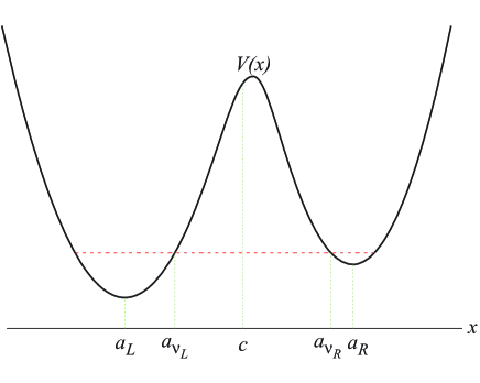
Figure 1: An asymmetric double-well potential $V(x)$ and the classical turning points $a_{\nu_{L}}$ and $a_{\nu_{R}}$. We assume that $V(x)$ is quadratic around its minima at $x=a_{L}$ and at $x=a_{R}$ with angular frequencies $\omega_{L}$ and $\omega_{R}$, respectively.

As we are interested in the barrier penetration, we restrict our attention on non-negative $\nu_{L}$ and $\nu_{R}$. By introducing

$$z_{i}=\frac{\sqrt{2}(x-a_{i})}{l_{i}},$$ (4)

with

$$l_{i}=\sqrt{{\hbar}\over{m\omega_{i}}},$$ (5)

we rewrite Eq. (3) as

$$\frac{d^{2}\psi}{dz_{i}^{2}}+\left(\nu_{i}+\frac{1}{2}-\frac{z_{i}^{2}}{4}\right)\psi=0.$$ (6)

The solutions of Eq. (6) are parabolic cylinder functions and we write the wave function $\psi(x)$ as

$$\psi_{L}(x)=C_{L}D_{\nu_{L}}(-z_{L})=C_{L}D_{\nu_{L}}\left(\frac{\sqrt{2}(a_{L}-x)}{l_{L}}\right)$$ (7)

and

$$\psi_{R}(x)=C_{R}D_{\nu_{R}}(z_{R})=C_{R}D_{\nu_{R}}\left(\frac{\sqrt{2}(x-a_{R})}{l_{R}}\right)$$ (8)

around the minima of the left-hand well and right-hand well, respectively, with constant $C_{L}$ and $C_{R}$ . The choice of the solution in Eq. ($\ref{pcfl})$ (in Eq. (8)) is made bearing in mind that we wish to construct a normalizable wave function so that $\int_{-\infty}^{a_{L}}|\psi_{L}(x)|^{2}dx$ ($\int_{a_{R}}^{\infty}|\psi_{R}(x)|^{2}dx$) is finite if we suppose the expression of $\psi_{L}(x)$ ($\psi_{R}(x)$) is valid for $x<a_{L}$ ($x>a_{R}$).

$D_{\alpha}(z)$ of Whittaker can be expressed in terms of other parabolic cylinder functions $U$ and $V$ as [19]

$$D_{\alpha}(z)=\cos(\alpha\pi)U(-\alpha-\frac{1}{2},-z)+\frac{\pi}{\Gamma(-\alpha)}V(-\alpha-\frac{1}{2},-z).$$ (9)

Equation (9) can be used to find the asymptotic expansion for $|z|\gg|\alpha|$

$$D_{\alpha}(z)~{} \sim ~{}\cos(\alpha\pi)\exp\left(-\frac{z^{2}}{4}\right)|z|^{\alpha}\left[1-\frac{\alpha(\alpha-1)}{2z^{2}}+\cdots\right]$$ (10)

$$~{}+\frac{\sqrt{2\pi}}{\Gamma(-\alpha)|z|^{\alpha+1}}\exp\left(\frac{z^{2}}{4}\right)\left[1+\frac{(\alpha+1)(\alpha+2)}{2z^{2}}+\cdots\right]$$

which is completely valid only for $z$ real and negative [19]. Using the relation

$$\Gamma(-\alpha)=-\frac{\pi}{\alpha!\sin(\alpha\pi)},$$

Eq. (10) is then rewritten as (see also Ref. [20])

$$D_{\alpha}(z)~{} \sim ~{}\cos(\alpha\pi)|z|^{\alpha}\exp\left(-\frac{z^{2}}{4}\right)\left[1-\frac{\alpha(\alpha-1)}{2z^{2}}+\cdots\right]$$ (11)

$$~{}-\frac{\sin(\alpha\pi)\alpha!}{|z|^{\alpha+1}}\sqrt{\frac{2}{\pi}}\exp\left(\frac{z^{2}}{4}\right)\left[1+\frac{(\alpha+1)(\alpha+2)}{2z^{2}}+\cdots\right].$$

In the quadratic region of the left-hand well satisfying $\sqrt{2}(x-a_{L})\gg\nu_{L}l_{L}$, using Eqs. (7) and (11), we obtain

$$\psi_{L}(x)\simeq C_{L}\cos(\nu_{L}\pi)\left(\frac{\sqrt{2}(x-a_{L})}{l_{L}}\right)^{\nu_{L}}e^{-\frac{(x-a_{L})^{2}}{2l_{L}^{2}}}$$ (12)

$$-C_{L}\sin(\nu_{L}\pi)\nu_{L}!\sqrt{\frac{2}{\pi}}\left(\frac{l_{L}}{\sqrt{2}(x-a_{L})}\right)^{\nu_{L}+1}e^{\frac{(x-a_{L})^{2}}{2l_{L}^{2}}}.$$

In the region of the right-hand well of $\sqrt{2}(a_{R}-x)\gg\nu_{R}l_{R}$, using Eqs. (8) and (11), we also have

$$\psi_{R}(x)\simeq C_{R}\cos(\nu_{R}\pi)\left({\sqrt{2}(a_{R}-x)\over l_{R}}\right)^{\nu_{R}}e^{-\frac{(x-a_{R})^{2}}{2l_{R}^{2}}}$$ (13)

$$-C_{R}\sin(\nu_{R}\pi)\nu_{R}!\sqrt{\frac{2}{\pi}}\left(\frac{l_{R}}{\sqrt{2}(a_{R}-x)}\right)^{\nu_{R}+1}e^{\frac{(x-a_{R})^{2}}{2l_{R}^{2}}}.$$

To be precise, in obtaining Eqs. (12) and (13), we have assumed the existence of certain numbers $N_{L}~{}(\gg\nu_{L})$ and $N_{R}~{}(\gg\nu_{R})$ such that the potential is quadratic in the regions $a_{L}\leq x\leq a_{L}+N_{L}l_{L}$ and $a_{R}-N_{R}l_{R}\leq x\leq a_{R}$. We note that, in Eq. (12), the magnitude of the ratio of the first term to the second one at $x=a_{L}+N_{L}l_{L}$ is $\sqrt{\frac{\pi}{2}}\frac{1}{\nu_{L}!}|\frac{\cos(\nu_{L}\pi)}{\sin(\nu_{L}\pi)}|(\sqrt{2}N_{L})^{2\nu_{L}+1}e^{-N_{L}^{2}},$ so that, if $\frac{1}{|\sin(\nu_{L}\pi)|}$ is moderate(not exponentially large), the magnitude of the first term for $N_{L}$ large is exponentially small compared to that of the second term when $x\gtrsim a_{L}+N_{L}l_{L}$. Likewise, in Eq. (13), if $N_{R}$ is large and $\frac{1}{|\sin(\nu_{R}\pi)|}$ is moderate, the second term is dominant over the first one for $x\lesssim a_{R}-N_{R}l_{R}$.

In the classically forbidden region between the wells, with a point $c$ satisfying $a_{L}<c<a_{R}$, the WKB approximation to an eigenfunction is written as

$$\psi_{WKB}(x)=A\sqrt{\frac{\hbar}{p(x)}}\exp\left(\int_{c}^{x}\frac{p(y)}{\hbar}dy\right)+B\sqrt{\frac{\hbar}{p(x)}}\exp\left(-\int_{c}^{x}\frac{p(y)}{\hbar}dy\right),$$ (14)

where $p(x)$ is defined as

$$p(x)=\sqrt{2m[V(x)-E]}.$$ (15)

We here define the classical turning points $a_{\nu_{L}}$ and $a_{\nu_{R}}$ satisfying $a_{L}<a_{\nu_{L}}<c<a_{\nu_{R}}<a_{R}$ (see Fig. 1) and

$$E=V(a_{\nu_{L}})=V(a_{\nu_{R}}).$$ (16)

In the region of quadratic potential near the left minimum, by introducing

$$W_{L}(\nu_{L}) = \int_{a_{\nu_{L}}}^{x}\frac{p(y)}{\hbar}dy=\int_{a_{\nu_{L}}}^{x}\sqrt{\frac{(a_{L}-y)^{2}}{l_{L}^{2}}-2\nu_{L}-1}~{}dy$$ (17)

$$= \int_{\sqrt{2\nu_{L}+1}}^{\frac{-a_{L}+x}{l_{L}}}\sqrt{z^{2}-2\nu_{L}-1}~{}dz$$ (18)

for $x>a_{\nu_{L}}$, we have the asymptotic expansion

$$W_{L}(\nu_{L}) = \frac{(-a_{L}+x)^{2}}{2l_{L}^{2}}-\frac{1}{2}(\nu_{L}+\frac{1}{2})$$ (20)

$$+(\nu_{L}+\frac{1}{2})\ln\frac{\sqrt{2}(-a_{L}+x)}{l_{L}\sqrt{\nu_{L}+\frac{1}{2}}}+O\left(\frac{l_{L}^{2}(\nu_{L}+\frac{1}{2})}{(-a_{L}+x)^{2}}\right).$$

With

$$\int_{c}^{x}\frac{p(y)}{\hbar}dy=\int_{c}^{a_{\nu_{L}}}\frac{p(y)}{\hbar}dy+W_{L}(\nu_{L}),$$

we then find

$$\psi_{WKB}(x)$$ (21)

$$\simeq A\frac{\sqrt{l_{L}}}{\pi^{\frac{1}{4}}}\sqrt{\nu_{L}!g_{\nu_{L}}}\left(\frac{l_{L}}{\sqrt{2}(x-a_{L})}\right)^{\nu_{L}+1}\exp\left(\frac{(-a_{L}+x)^{2}}{2l_{L}^{2}}-\int_{a_{\nu_{L}}}^{c}\frac{p(y)}{\hbar}dy\right)\phantom{\hskip 11.38092pt}$$ (22)

$$~{}~{}+B\frac{(4\pi)^{\frac{1}{4}}\sqrt{l_{L}}}{\sqrt{\nu_{L}!g_{\nu_{L}}}}\left(\frac{\sqrt{2}(x-a_{L})}{l_{L}}\right)^{\nu_{L}}\exp\left(-\frac{(-a_{L}+x)^{2}}{2l_{L}^{2}}+\int_{a_{\nu_{L}}}^{c}\frac{p(y)}{\hbar}dy\right)~{}$$ (23)

for $\sqrt{2}(-a_{L}+x)\gg l_{L}\sqrt{2\nu_{L}+1}$, where

$$g_{k}=\frac{\sqrt{2\pi}}{k!}\left(k+\frac{1}{2}\right)^{k+\frac{1}{2}}e^{-k-\frac{1}{2}}.$$ (24)

Matching this expression of $\psi_{WKB}(x)$ onto the asymptotic form of $\psi_{L}(x)$ in the overlap region, we have

$$A = -\sin(\nu_{L}\pi)\frac{\sqrt{2\nu_{L}!}}{{\pi^{\frac{1}{4}}\sqrt{l_{L}g_{\nu_{L}}}}}\exp\left(\int_{a_{\nu_{L}}}^{c}\frac{p(y)}{\hbar}dy\right)C_{L},$$ (25)

$$B = \cos(\nu_{L}\pi)\frac{\sqrt{\nu_{L}!g_{\nu_{L}}}}{(4\pi)^{\frac{1}{4}}\sqrt{l_{L}}}\exp\left(-\int_{a_{\nu_{L}}}^{c}\frac{p(y)}{\hbar}dy\right)C_{L}.$$ (26)

In passing, we note that the form of $g_{k}$ first appears in Ref. [21] from the comparison between an exact eigenfunction and the corresponding semiclassical wave function for the harmonic oscillator. For a plane pendulum in quantum mechanics described by Mathieu’s equation, it is well-known that, in the limit of low probability for barrier penetration, the correct asymptotic mathematical expression for the width of the $k$-th energy band ($k$-th stable region) is given by the product of $g_{k-1}$ and the result obtained from the semiclassical calculation [10] at the leading order [11].

With the notation

$$W_{R}(\nu_{R}) = \int_{x}^{a_{\nu_{R}}}\frac{p(y)}{\hbar}dy=\int_{x}^{a_{\nu_{R}}}\sqrt{\frac{(a_{R}-y)^{2}}{l_{R}^{2}}-2\nu_{R}-1}~{}dy$$ (27)

$$= \int_{\sqrt{2\nu_{R}+1}}^{\frac{a_{R}-x}{l_{R}}}\sqrt{z^{2}-2\nu_{R}-1}~{}dz,$$ (28)

using the asymptotic relation

$$W_{R}(\nu_{R})\simeq\frac{(a_{R}-x)^{2}}{2l_{R}^{2}}-\frac{1}{2}(\nu_{R}+\frac{1}{2})+(\nu_{R}+\frac{1}{2})\ln\frac{\sqrt{2}(a_{R}-x)}{l_{R}\sqrt{\nu_{R}+\frac{1}{2}}},$$ (29)

in the quadratic-potential region around the right minimum satisfying $\sqrt{2}(a_{R}-x)\gg\l_{R}\sqrt{2\nu_{R}+1}$, we have

$$\psi_{WKB}(x)$$ (30)

$$\simeq A\frac{(4\pi)^{\frac{1}{4}}\sqrt{l_{R}}}{\sqrt{\nu_{R}!g_{\nu_{R}}}}\left(\frac{\sqrt{2}(a_{R}-x)}{l_{R}}\right)^{\nu_{R}}\exp\left(-\frac{(a_{R}-x)^{2}}{2l_{R}^{2}}+\int_{c}^{a_{\nu_{R}}}\frac{p(y)}{\hbar}dy\right)\phantom{\hskip 34.14322pt}$$ (31)

$$~{}+B\frac{\sqrt{l_{R}\nu_{R}!g_{\nu_{R}}}}{\pi^{\frac{1}{4}}}\left(\frac{l_{R}}{\sqrt{2}(a_{R}-x)}\right)^{\nu_{R}+1}\exp\left(\frac{(a_{R}-x)^{2}}{2l_{R}^{2}}-\int_{c}^{a_{\nu_{R}}}\frac{p(y)}{\hbar}dy\right).$$ (32)

Comparing $\psi_{WKB}(x)$ and $\psi_{R}(x)$ in the overlap region, we obtain

$$A = \cos(\nu_{R}\pi)\frac{\sqrt{\nu_{R}!g_{\nu_{R}}}}{(4\pi)^{\frac{1}{4}}\sqrt{l_{R}}}\exp\left(-\int_{c}^{a_{\nu_{R}}}\frac{p(y)}{\hbar}dy\right)C_{R},$$ (33)

$$B = -\sin(\nu_{R}\pi)\frac{\sqrt{2\nu_{R}!}}{\pi^{\frac{1}{4}}\sqrt{l_{R}g_{\nu_{R}}}}\exp\left(\int_{c}^{a_{\nu_{R}}}\frac{p(y)}{\hbar}dy\right)C_{R}.$$ (34)

For the reasons given after Eq. (13), for large $N_{L}$ and moderate $\frac{1}{|\sin(\nu_{L}\pi)|}$, the first term in Eq. (12) is subleading in the overlap region, which means that Eq. (26) comes from the comparison between exponentially small terms compared to the leading ones. For the WKB approximation, it has been discussed that the accuracy of the approximation is not such as to allow the retention in the wave function of exponentially small terms superimposed on exponentially large ones [12]. This implies that, while Eq. (25) is valid within the approximation, this approximation does not provide the validity of Eq. (26) for large $N_{L}$ and moderate $\frac{1}{|\sin(\nu_{L}\pi)|}$. On the other hand, in the limit of $\nu_{L}\rightarrow n_{L}$ with a non-negative integer $n_{L}$, as the fact

$$D_{n_{L}}(z)=2^{-\frac{n_{L}}{2}}e^{-\frac{z^{2}}{4}}H_{n_{L}}\left(\frac{z}{\sqrt{2}}\right)$$ (35)

implies, $\psi_{L}(x)$ reduces to $(-)^{n_{L}}C_{L}\pi^{\frac{1}{4}}\sqrt{n_{L}!l_{L}}\psi_{n_{L}}^{sho}(a_{L};x)$, with the $n_{L}$th excited state harmonic oscillator wave function

$$\psi_{n_{L}}^{sho}(a_{L};x)=\frac{1}{\pi^{\frac{1}{4}}\sqrt{2^{n_{L}}n_{L}!l_{L}}}H_{n_{L}}\left(\frac{x-a_{L}}{l_{L}}\right)e^{-\frac{(x-a_{L})^{2}}{2l_{L}^{2}}}$$

$$~{}=\frac{1}{\pi^{\frac{1}{4}}\sqrt{2^{n_{L}}n_{L}!l_{L}}}e^{-\frac{(x-a_{L})^{2}}{2l_{L}^{2}}}\left(\frac{2(x-a_{L})}{l_{L}}\right)^{n_{L}}[1-\frac{n_{L}(n_{L}-1)l_{L}^{2}}{4(x-a_{L})^{2}}+\cdots],\phantom{\hskip 19.91684pt}$$ (36)

where $H_{n_{L}}$ denotes the $n_{L}$th order Hermite polynomial. Thus, if $\nu_{L}$ is in the (Hermite-Gaussian) limit of $\frac{1}{|\sin(\nu_{L}\pi)|}\rightarrow\infty$, Eq. (26) is valid while the WKB method may not provide the validity of Eq. (25). Likewise, for large $N_{R}$, Eq. (34) is valid if $\frac{1}{|\sin(\nu_{R}\pi)|}$ is moderate, and Eq. (33) is valid if $\nu_{R}$ is in the limit of $\frac{1}{|\sin(\nu_{R}\pi)|}\rightarrow\infty$, in the approximations.

Here, we assume that the potential is quadratic in the region $|x-a_{L}|\leq N_{L}l_{L}$ with the large $N_{L}$; for small $n_{L}$,

$$\epsilon_{L}=V(a_{L})+(n_{L}+\frac{1}{2})\hbar\omega_{L}$$ (37)

is thus approximately an eigenvalue of the double-well system so that, for the corresponding eigenvalue $E$, $\nu_{L}\simeq n_{L}$. For this eigenvalue,

$$(-)^{n_{L}}C_{L}\pi^{\frac{1}{4}}\sqrt{n_{L}!l_{L}}\psi_{n_{L}}^{sho}(a_{L};x)$$

is a good approximation to $\psi_{L}(x)$, which implies that Eq. (26) is valid. Similarly, for a small non-negative integer $n_{R}$,

$$\epsilon_{R}=V(a_{R})+(n_{R}+\frac{1}{2})\hbar\omega_{R}$$ (38)

is approximately an eigenvalue of the double-well system, and for the corresponding eigenvalue Eq. (33) is valid with $\nu_{R}\simeq n_{R}$.

For $\nu_{L}\simeq n_{L}$ with moderate $\frac{1}{|\sin(\nu_{R}\pi)|}$, using Eqs. (26) and (34) which are (approximtely) valid in this case, we find

$$\frac{C_{L}}{C_{R}}=-\frac{2\sin(\pi\nu_{R})}{\cos(\pi\nu_{L})}\sqrt{\frac{\nu_{R}!l_{L}}{\nu_{L}!l_{R}}}\frac{1}{\sqrt{g_{\nu_{L}}g_{\nu_{R}}}}~{}e^{\int_{a_{\nu_{L}}}^{a_{\nu_{R}}}\frac{p(y)}{\hbar}dy}.$$ (39)

For $\nu_{R}\simeq n_{R}$ with moderate $\frac{1}{|\sin(\nu_{L}\pi)|}$, using Eqs. (25) and ($\ref{ACR})$, likewise, we have

$$\frac{C_{L}}{C_{R}}=-\frac{\cos(\pi\nu_{R})}{2\sin(\pi\nu_{L})}\sqrt{\frac{\nu_{R}!l_{L}}{\nu_{L}!l_{R}}}\sqrt{g_{\nu_{L}}g_{\nu_{R}}}~{}e^{-\int_{a_{\nu_{L}}}^{a_{\nu_{R}}}\frac{p(y)}{\hbar}dy}.$$ (40)

If $\nu_{L}\simeq n_{L}$ with moderate $\frac{1}{|\sin(\nu_{R}\pi)|}$, while the validity of Eq. (40) as well as that of Eq. ($\ref{ACR})$ is not provided by the the WKB approximation, Eq. (39) is valid within the approximations to show that $|C_{L}|\gg|C_{R}|$. The ratio $R(\nu_{L},\nu_{R})$ of the probability of the particle being in the classically allowed region of the left-hand well to that of the right-hand well is given as

$$R(\nu_{L},\nu_{R})=\bigg{|}\frac{C_{L}}{C_{R}}\bigg{|}^{2}\frac{l_{L}}{l_{R}}\frac{\int_{-\sqrt{4\nu_{L}+2}}^{\sqrt{4\nu_{L}+2}}[D_{\nu_{L}}(z_{L})]^{2}dz_{L}}{\int_{-\sqrt{4\nu_{R}+2}}^{\sqrt{4\nu_{R}+2}}[D_{\nu_{R}}(z_{R})]^{2}dz_{R}}.$$

Since $D_{\alpha}(z)$ is an entire function of $z$ with $D_{\alpha}(0)=\frac{2^{\frac{\alpha}{2}}}{\sqrt{\pi}}(\frac{\alpha-1}{2})!\cos(\frac{\alpha}{2}\pi)$ and $\frac{dD_{\alpha}(z)}{dz}|_{z=0}=\frac{2^{\frac{\alpha+1}{2}}}{\sqrt{\pi}}\left(\frac{\alpha}{2}\right)!\sin(\frac{\alpha}{2}\pi)$ [15], for the large $N_{L},$ $N_{R}$ and moderate $\frac{1}{|\sin(\nu_{R}\pi)|},$ Eq. (39) thus implies that the eigenstate is primarily localized in the left-hand well with negligible magnitude for $x>c$. We note that, in the expression of $\psi_{R}(x)$ given in Eq. (13), the second term whose magnitude decreases rapidly when $z_{R}$ increases from $-\sqrt{2}N_{R}$ towards $-\nu_{R}$ is dominant over the first one in the asymptotic region for moderate $\frac{1}{|\sin(\nu_{R}\pi)|}$, in accordance with the localization. This localization in turn suggests that the corresponding eigenstate is non-degenerate. Indeed, localized non-degenerate eigenstates have been found numerically in various asymmetric double-well systems without necessarily assuming parabolicities of the wells [5, 6]. Likewise, for the non-degenerate eigenstate of $E\approx\epsilon_{R}$ with moderate $\frac{1}{|\sin(\nu_{L}\pi)|}$, Eq. (40) shows that the eigenstate is primarily localized in the right-hand well.

If $\epsilon_{L}\approx\epsilon_{R}$ so that both Eqs. (39) and (40) are valid, they give rise to the quantization condition for the energy levels:

$$\tan(\pi\nu_{L})\tan(\pi\nu_{R})=\frac{1}{4}g_{\nu_{L}}g_{\nu_{R}}\exp\left(-2\int_{a_{\nu_{L}}}^{a_{\nu_{R}}}\frac{p(y)}{\hbar}dy\right).$$ (41)

We note that quantization formula analogous to Eq. (41) has been found in a semiclassical analysis for a general double-well potential problem [16, 17]; in these previous derivations, however, since the wells are not assumed to be parabolic, the equation has been given in terms of the action integrals on the left-hand side and without the prefactor $g_{\nu_{L}}g_{\nu_{R}}$ on the right-hand side [16, 17]. From its derivation given here, we note that Eq. (41) is valid only when $\nu_{L}\simeq n_{L}$ and $\nu_{R}\simeq n_{R}$; further, in this equation, $\frac{1}{|\sin(\nu_{R}\pi)|}$ and $\frac{1}{|\sin(\nu_{R}\pi)|}$ are implicitly assumed to be moderately large so that one term is not exponentially dominant over the other in the overlap region in Eqs. (12) and (13), for the validity of Eqs. (25) and (34) (see also next section).

For further analyses of the quantization condition, with the constants $\delta_{n_{L}},~{}\delta_{n_{R}}$ satisfying

$$\epsilon_{L}+\hbar\omega_{L}\delta_{n_{L}}=\epsilon_{R}+\hbar\omega_{R}\delta_{n_{R}},$$ (42)

we define

$$\triangle\epsilon=\epsilon_{L}-\epsilon_{R}=\hbar(\delta_{n_{R}}\omega_{R}-\delta_{n_{L}}\omega_{L}),$$ (43)

to rewrite $\nu_{L}$, $\nu_{R}$ in Eq. (1) as

$$\nu_{L}=n_{L}+\delta_{n_{L}}+\delta_{L},~{}~{}~{}~{}\nu_{R}=n_{R}+\delta_{n_{R}}+\frac{\omega_{L}}{\omega_{R}}\delta_{L},$$ (44)

with a constant $\delta_{L}$ ($|\delta_{L}|\ll 1$). Equation (41) is then approximated as

$$(\delta_{L}+\frac{\omega_{R}}{\omega_{L}}\delta_{n_{R}})(\delta_{L}+\delta_{n_{L}})=\frac{\omega_{R}}{\omega_{L}}\left[\frac{\sqrt{{g_{n_{L}}g_{n_{R}}}}}{2\pi}\exp\left(-\int_{a_{n_{L}}}^{a_{n_{R}}}\frac{p(y)}{\hbar}dy\right)\right]^{2}.$$ (45)

Two real roots of the quadratic equation of Eq. (45) for $\delta_{L}$ give two energy eigenvalues $E_{\pm}$ .

For the degenerate left and right states of $\epsilon_{R}=\epsilon_{L}$, using $\delta_{n_{L}}=\delta_{n_{R}}=0$, we obtain the splitting ${\it\Delta}$ $(=2|\delta_{L}|\hbar\omega_{L})$ between the two energy eigenvalues:

$${\it\Delta}=\frac{\hbar}{\pi}\sqrt{g_{n_{L}}g_{n_{R}}\omega_{L}\omega_{R}}\exp\left(-\int_{a_{n_{L}}}^{a_{n_{R}}}\frac{p(y)}{\hbar}dy\right)$$ (46)

which exactly agrees with the result given in Ref. [6]. Using Eq. (44), $C_{L}/C_{R}$ can be approximated from Eqs. (39) (or (40)) as

$$\frac{C_{L}}{C_{R}}=\pm(-1)^{n_{L}+n_{R}}\sqrt{\frac{n_{R}!l_{R}}{n_{L}!l_{L}}}$$ (47)

for $E=E_{\mp}$. The following formula for an integer $n$ [15]

$$\int_{-\infty}^{\infty}\{D_{n}(z)\}^{2}dz=\sqrt{2\pi}n!,$$

and Eq. (47) then imply that the left-right amplitude ratio is approximately unity (that is, $\int_{-\infty}^{c}|\psi(x)|^{2}dx\simeq\int_{c}^{\infty}|\psi(x)|^{2}dx$) for $E=E_{\pm}$.

For $\triangle\epsilon\neq 0$, with the two roots $\delta_{L_{+}}$ and $\delta_{L_{-}}$ of Eq. (45), we find the eigenvalues

$$E_{\pm} = \hbar\omega_{L}\left[n_{L}+\delta_{n_{L}}+\frac{1}{2}+\frac{1}{2}\left\{(\delta_{L_{+}}+\delta_{L_{-}})\pm(\delta_{L_{+}}-\delta_{L_{-}})\right\}\right]+V(a_{L})$$ (48)

$$= \hbar\omega_{L}\left[n_{L}+\frac{1}{2}\left(1+\delta_{n_{L}}-\frac{\omega_{R}}{\omega_{L}}\delta_{n_{L}}\right)\right]+V(a_{L})\pm\frac{1}{2}\sqrt{(\triangle\epsilon)^{2}+{\it\Delta}^{2}}$$

$$= \frac{1}{2}(\epsilon_{L}+\epsilon_{R})\pm\frac{1}{2}\sqrt{(\triangle\epsilon)^{2}+{\it\Delta}^{2}},$$

to get the energy splitting

$$\triangle E=E_{+}-E_{-}=\sqrt{(\triangle\epsilon)^{2}+{\it\Delta}^{2}}.$$ (49)

In view of the discussions on two-level systems (see, e.g., Ref. [22]), Eq. (49) suggests that, for $\triangle E\ll\hbar\omega_{L}$ and $\triangle E\ll\hbar\omega_{R}$, we can confine ourselves to a two-dimensional subspace described by the eigenfunctions corresponding to the eigenvalues $E=E_{\pm}$ as a first approximation.

3 Two-level approximation and energy splitting

For a two-level approximation, we hypothesize two approximate solutions to the Schrödinger equation $\tilde{\psi}_{L}(x)$ and $\tilde{\psi}_{R}(x)$ which are primarily localized with energy $E$ in the left-hand and right-hand wells, respectively. For $\tilde{\psi}_{L}(x)$ with $E\simeq\epsilon_{L}$, we naturally approximate $\tilde{\psi}_{L}(x)$ by $\psi_{n_{L}}^{sho}(a_{L};x)$ near $x=a_{L}$, which will be more accurate in the (Hermite-Gaussian) limit of $E\rightarrow\epsilon_{L}$ ($\nu_{L}\rightarrow n_{L}$). The pertinent WKB wave function in the forbidden region between the wells is then

$$\psi_{WKB}^{L}(x)=N_{L}\sqrt{\frac{\hbar}{p(x)}}e^{-\int_{c}^{x}\frac{p(y)}{\hbar}dy}$$ (50)

the amplitude of which decreases as $x$ increases. In the region of quadratic potential satisfying $\sqrt{2}(-a_{L}+x)\gg l_{L}\sqrt{2n_{L}+1}$, using Eq. (20), we have

$$\psi_{WKB}^{L}(x)=N_{L}\sqrt{\frac{\hbar}{p(x)}}\exp\left(\int_{a_{n_{L}}}^{c}\frac{p(y)}{\hbar}dy-W_{L}(n_{L})\right)\phantom{\hskip 93.89418pt}$$ (51)

$$\simeq N_{L}\frac{(4\pi)^{\frac{1}{4}}\sqrt{l_{L}}}{\sqrt{n_{L}!g_{n_{L}}}}\left(\frac{\sqrt{2}(x-a_{L})}{l_{L}}\right)^{n_{L}}\exp\left(-\frac{(-a_{L}+x)^{2}}{2l_{L}^{2}}+\int_{a_{n_{L}}}^{c}\frac{p(y)}{\hbar}dy\right).$$ (52)

Requiring that this asymptotic form of $\psi_{WKB}^{L}(x)$ matches onto that of $\psi_{n_{L}}^{sho}(a_{L};x)$ in the forbidden region near the turning point, we find

$$N_{L}=\sqrt{\frac{g_{n_{L}}}{2\pi}}\frac{1}{l_{L}}\exp\left[-\int_{a_{n_{L}}}^{c}\frac{p(y)}{\hbar}dy\right],$$ (53)

and thus [13]

$$\psi_{WKB}^{L}(x)=\sqrt{\frac{m\omega_{L}g_{n_{L}}}{2\pi p(x)}}~{}e^{-\int_{a_{n_{L}}}^{x}\frac{p(y)}{\hbar}dy}.$$ (54)

Since we are considering $\tilde{\psi}_{L}(x)$ primarily localized in the left-hand well, we will take $\tilde{\psi}_{L}(x)=0$ for $x>a_{R}-N_{R}l_{R}$ in further use. For $\tilde{\psi}_{R}(x)$ with $E\simeq\epsilon_{R}$, the pertinent WKB wave function in the forbidden region between the wells is

$$\psi_{WKB}^{R}(x)=N_{R}\sqrt{\frac{\hbar}{p(x)}}e^{\int_{c}^{x}\frac{p(y)}{\hbar}dy}.$$ (55)

Requiring that the asymptotic form of $\psi_{WKB}^{R}(x)$ matches onto that of $\psi_{n_{R}}^{sho}(a_{R};x)$ in the region of quadratic potential satisfying $\sqrt{2}(a_{R}-x)\gg l_{R}\sqrt{2n_{R}+1}$, where $\psi_{n_{R}}^{sho}(a_{R};x)$ is defined by the replacement of the subscript $L$ by $R$ in Eq. (36), we have

$$N_{R}=(-1)^{n_{R}}\sqrt{\frac{g_{n_{R}}}{2\pi}}\frac{1}{l_{R}}\exp\left[-\int_{c}^{a_{n_{R}}}\frac{p(y)}{\hbar}dy\right].$$ (56)

The factor $(-1)^{n_{R}}$ in Eq. (56) is due to the negativity of the harmonic oscillator wave function $\psi_{n_{R}}^{sho}(a_{R};x)$ of odd $n_{R}$ in the limit of $x-a_{R}\ll-l_{R}$.

Assuming that $\epsilon_{L}$ and $\epsilon_{R}$ are close together and very different from the energy eigenvalues of all other states of the system, we may restrict our attention on the two-dimensional subspace spanned by $\tilde{\psi}_{L}(x)$ and $\tilde{\psi}_{R}(x)$ [22]. For simplicity we start with the case of $\epsilon_{L}=\epsilon_{R}=E_{0}$ in which all the diagonal elements of the $2\times 2$ Hamiltonian matrix in the subspace are $E_{0}$, and the off-diagonal elements $\int_{-\infty}^{\infty}\tilde{\psi}_{L}^{*}(x)H\tilde{\psi}_{R}(x)$ and $\int_{-\infty}^{\infty}\tilde{\psi}_{R}^{*}(x)H\tilde{\psi}_{L}(x)$ are equal to each other since we have taken $\tilde{\psi}_{L}(x)$ and $\tilde{\psi}_{R}(x)$ to be real. It is easy to find that the eigenfunctions corresponding to the energy eigenvalues $E_{0}\pm\frac{\tilde{\it\Delta}}{2}$ in the subspace are written as

$$\tilde{\psi}_{\pm}(x)=\frac{1}{\sqrt{2}}\left(\tilde{\psi}_{L}(x)\mp(-1)^{n_{R}}\tilde{\psi}_{R}(x)\right),$$ (57)

where

$$\tilde{\it\Delta}=2\times(-1)^{n_{R}+1}\int_{-\infty}^{\infty}\tilde{\psi}_{L}(x)H\tilde{\psi}_{R}(x).$$ (58)

To find an explicit expression of $\tilde{\it\Delta}$, as in Ref. [4], we multiply the Schrödinger equation (2) for $\tilde{\psi}_{+}(x)$ with energy $E_{0}+\frac{\tilde{\it\Delta}}{2}$ by $\tilde{\psi}_{-}(x)$, and the equation for $\tilde{\psi}_{-}(x)$ with energy $E_{0}-\frac{\tilde{\it\Delta}}{2}$ by $\tilde{\psi}_{+}(x)$. Subtracting the two resulting expressions and integrating over $x\in[c,\infty)$, with the facts

$$\int_{c}^{\infty}(\tilde{\psi}_{R}(x))^{2}dx\simeq 1,~{}~{}\int_{c}^{\infty}(\tilde{\psi}_{L}(x))^{2}dx\simeq 0,~{}~{}{\rm and}~{}\int_{c}^{\infty}\tilde{\psi}_{L}(x)\tilde{\psi}_{R}(x)dx\simeq 0$$ (59)

which are given by the definitions of $\tilde{\psi}_{L}(x)$ and $\tilde{\psi}_{R}(x)$, we find

$$\tilde{\it\Delta}\simeq(-1)^{n_{R}}\frac{2\hbar^{2}}{m}N_{L}N_{R}.$$ (60)

With the explicit expressions given in Eqs. (53) and (56), it is easy to check that $\tilde{\it\Delta}$ reduces to ${\it\Delta}$ of Eq. (46). Moreover, using the expressions of $A$ and $B$ in Eqs. (25) and (26) (or, in Eqs. (33) and (34)), if $\nu_{L}=n_{L}\pm\frac{\it\Delta}{2\hbar\omega_{L}}$ and $\nu_{R}=n_{R}\pm\frac{\it\Delta}{2\hbar\omega_{R}}$, we find that

$$\frac{B}{A}\simeq\mp(-1)^{n_{R}}\frac{N_{L}}{N_{R}}.$$ (61)

Equation (61) implies that $\tilde{\psi}_{\pm}(x)$ reduces to $\psi(x)$ for $E=E_{\pm}$ up to normalization constants in the forbidden region between the wells, to show that this two-level description is indeed equivalent to the wave function approach of the previous section, for $\triangle\epsilon=0$.

In the (Hermite-Gaussian) limit of $\nu_{L}\rightarrow n_{L}$ Eq. (53) is equal to Eq. (26) with $B=N_{L}$ and $C_{L}=(-1)^{n_{L}}\frac{1}{\pi^{\frac{1}{4}}\sqrt{n_{L}!l_{L}}}$, and in the limit of $\nu_{R}\rightarrow n_{R}$ Eq. (56) is equal to Eq. (33) when $A=N_{R}$ and $C_{R}=\frac{1}{\pi^{\frac{1}{4}}\sqrt{n_{R}!l_{R}}}$. For the low-lying states, the approximation of $\tilde{\psi}_{L}(x)$ ($\tilde{\psi}_{R}(x)$) by $\psi_{n_{L}}^{sho}(a_{L};x)$ ($\psi_{n_{R}}^{sho}(a_{R};x))$ near the turning point would be more accurate in the limit of $\nu_{L}\rightarrow n_{L}$ ($\nu_{R}\rightarrow n_{R}$), while, as has been discussed in the previous section, the WKB method does not provide the validity of Eq. (25) (Eq. (34)) in the limit; indeed, neither Eq. (25) nor Eq. (34) has appeared in obtaining Eq. (60). Nevertheless, the fact $\tilde{\it\Delta}\simeq{\it\Delta}$ may suggest that when $\nu_{L}\simeq n_{L}$ and $\nu_{R}\simeq n_{R}$, $\nu_{L}$ and $\nu_{R}$ adjust themselves so that $\frac{1}{|\sin(\nu_{L}\pi)|}$ and $\frac{1}{|\sin(\nu_{R}\pi)|}$ are moderately large and thus Eqs. (25) and (34) are in fact valid to render Dekker’s method applicable.

It is straightforward to extend the description to include the case of $\triangle\epsilon\neq 0$. Without losing generality, we assume $\triangle\epsilon>0$. In this case, the $2\times 2$ Hamiltonian matrix in the subspace spanned by $\tilde{\psi}_{L}(x)$ and $\tilde{\psi}_{R}(x)$ is

$$\left(\begin{array}[]{cc}\epsilon_{L}&(-1)^{n_{R}+1}\frac{\tilde{\it\Delta}}{2}\\ (-1)^{n_{R}+1}\frac{\tilde{\it\Delta}}{2}&\epsilon_{R}\end{array}\right)\phantom{\hskip 170.71652pt}$$ (64)

$$~{}~{}=\frac{\epsilon_{L}+\epsilon_{R}}{2}\left(\begin{array}[]{cc}1&0\\ 0&1\end{array}\right)+\frac{1}{2}\sqrt{(\triangle\epsilon)^{2}+{\tilde{\it\Delta}}^{2}}\left(\begin{array}[]{cc}\cos\theta&\sin\theta\\ \sin\theta&-\cos\theta\end{array}\right),$$ (69)

and the eigenfunctions $\psi_{\pm}(\theta;x)$ of the Hamiltonian corresponding to the eigenvalues $E_{\pm}$ of Eq. (48) are written as

$$\psi_{+}(\theta;x) = \cos(\frac{\theta}{2})\tilde{\psi}_{L}(x)+\sin(\frac{\theta}{2})\tilde{\psi}_{R}(x),$$ (70)

$$\psi_{-}(\theta;x) = (-1)^{n_{R}}\left[-\sin(\frac{\theta}{2})\tilde{\psi}_{L}(x)+\cos(\frac{\theta}{2})\tilde{\psi}_{R}(x)\right]$$ (71)

up to constant phases, where

$$\cos\theta=\frac{\triangle\epsilon}{\sqrt{(\triangle\epsilon)^{2}+{\tilde{\it\Delta}}^{2}}},~{}~{}\sin\theta=\frac{(-1)^{n_{R}+1}\tilde{\it\Delta}}{\sqrt{(\triangle\epsilon)^{2}+{\tilde{\it\Delta}}^{2}}}$$ (72)

with $-\frac{\pi}{2}<\theta<\frac{\pi}{2}$. The method described in Ref. [4] can also be used as follows;

$$\int_{c}^{\infty}[\psi_{-}(\theta;x)H\psi_{+}(\theta;x)-\psi_{+}(\theta;x)H\psi_{-}(\theta;x)]dx$$ (73)

$$=\sqrt{\triangle\epsilon)^{2}+{\tilde{\it\Delta}}^{2}}\int_{c}^{\infty}\psi_{-}(\theta;x)\psi_{+}(\theta;x)dx\simeq-\frac{\tilde{\it\Delta}}{2}$$ (74)

$$=-\frac{\hbar^{2}}{2m}\int_{c}^{\infty}\frac{d}{dx}\left[\psi_{-}(\theta;x)\frac{d}{dx}\psi_{+}(\theta;x)-\psi_{+}(\theta;x)\frac{d}{dx}\psi_{-}(\theta;x)\right]dx$$ (75)

$$=(-1)^{n_{R}}~{}\frac{\hbar^{2}}{2m}\int_{c}^{\infty}\frac{d}{dx}\left[\psi_{L}(x)\frac{d}{dx}\psi_{R}(x)-\psi_{R}(x)\frac{d}{dx}\psi_{L}(x)\right]dx$$ (76)

$$=(-1)^{n_{R}+1}~{}\frac{\hbar^{2}}{2m}\left[\psi_{L}(x)\frac{d}{dx}\psi_{R}(x)-\psi_{R}(x)\frac{d}{dx}\psi_{L}(x)\right]\bigg{|}_{x=c}$$ (77)

$$=(-1)^{n_{R}+1}\frac{\hbar^{2}}{m}N_{L}N_{R},$$ (78)

to show that the expression of $\tilde{\it\Delta}$ in Eq. (60) is still valid in this case. In obtaining the last equality in Eq. (78), we used the fact that $V(x)$ is differentiable at $x=c$. It is easy to check that, if we take the limit of $\theta\rightarrow(-1)^{n_{R}+1}\frac{\pi}{2}$, $\psi_{\pm}(\theta;x)$ reduce to $\tilde{\psi}_{\pm}(x)$ of $\triangle\epsilon=0$.

4 Concluding remarks

We have systematically applied Dekker’s method for the low-lying states of an asymmetric potential. While the method gives the quantization condition for two almost degenerate states which reproduces the energy splitting formula obtained through the two-level approach [6], for the other low-lying states it shows that the eigenstate is non-degenerate and primarily localized in one of the wells. Indeed, numerical studies with [5] or without parabolicity [6] implies that the low-lying eigenstate of an asymmetric double-well potential is either one of the two almost degenerate tunneling states or a localized non-degenerate state, in accordance with the analytic reasons given here. Though we have introduced $c$ satisfying $a_{L}+N_{L}l_{L}<c<a_{R}-N_{R}l_{R}$ during the derivations, the point $c$ appears neither in the quantization condition nor in $C_{L}/C_{R}$. This independence from the choice of $c$ implies that the splitting formula in Eqs. (46) and (49) would be applicable even when the potential barrier is not simply concave downwards. It would be interesting to test the splitting formula for the potential which is above $V(a_{n_{L}})$ $(=V(a_{n_{R}}))$ between $a_{n_{L}}$ and $a_{n_{R}}$ but has structures such as bumps and wells. Though numerical methods can be used for a specific one-dimensional potential problem to find the eigenvalues, however, we believe that the analytic result which is shown to be accurate for the low-lying states in the numerical calculations [6] would be of importance by itself. The evaluation of the energy splitting in a symmetric double-well potential is known to be closely related to that of widths of energy bands in a periodic potential [23], and it would be interesting if one could extend Dekker’s method to be applicable for a periodic problem.

References

• [1] R.J. Bemish, M.C. Chan, R.E. Miller, Chem. Phys. Lett. 251 (1996) 182.
• [2] J.P. Gordon, Phys. Rev. 99 (1955) 1253.
• [3] N. Noguchi, K. Komatsu, A. Shinozaki, K. Shinoda, H. Kagi, Spectrochim. Acta A 133 (2014) 509.
• [4] H. Dekker, Phys. Rev. A 35 (1987) 1825.
• [5] J.H. Weiner, S.T. Tse, J. Chem Phys. 74 (1981) 2419.
• [6] P.R. Johnson, W.T. Parsons, F.W. Strauch, J.R. Anderson, A.J. Dragt, C.J. Lobb, F.C. Wellstood, Phys. Rev. Lett. 94 (2005) 187004.
• [7] J. Koch, T.M. Yu, J. Gambetta, A.A. Houck, D.I. Schuster, J. Majer, A. Blais, M.H. Devoret, S.M. Girvin, R.J. Schoelkopf, Phys. Rev. A 76 (2007) 042319.
• [8] G. Catelani, R.J. Schoelkopf, M.H. Devoret, L.I. Glazman, Phys. Rev. B 84 (2011) 064517.
• [9] G. Blanch, 20. Mathieu Functions, in: M. Abramowitz, I.A. Stegun (Eds.), Handbook of Mathematical Functions with Formulas, Graphs, and Mathematical Tables, John Wiley & Sons, New York, 1972.
• [10] J.N.L. Connor, T. Uzer, R.A. Marcus, A.D. Smith, J. Chem. Phys. 80 (1984) 5095.
• [11] G. Wolf, Chapter 28 Mathieu Functions and Hill’s Equation, in: F.W.J. Olver, D.W. Lozier, R.F. Boisvert, C.W. Clark (Eds.), NIST Handbook of Mathematical Functions, Cambridge Univ. Press, New York, 2010, p. 661.
• [12] L.D. Landau, E.M. Lifshitz, Quantum Mechanics, third ed., Elsevier Butterworth-Heinemann, Amsterdam, 1977, pp. 166-185.
• [13] D.-Y. Song, Ann. Phys. 323 (2008) 2991; arXiv:1102.0083 (unpublished).
• [14] H. Dekker, Physica 146A (1987) 375.
• [15] E.T. Whittaker, G.N. Watson, A Course of Modern Analysis, fourth ed., Cambridge University Press, Cambridge, 1992.
• [16] N. Fröman, P.O. Fröman, U. Myhrman, and R. Paulsson, Ann. Phys. 74 (1972) 314;
N. Fröman, P.O. Fröman, Physical Problems Solved by the Phase-Integral Methods, Cambridge Univ. Press, Cambridge, 2002.
• [17] J.N.L. Connor, Chem. Phys. Lett. 4 (1969) 419.
• [18] G. Rastelli, Phys. Rev. A 86 (2012) 012106.
• [19] J.C.P. Miller, 19. Parabolic Cylinder Functions, in: M. Abramowitz, I.A. Stegun (Eds.), Handbook of Mathematical Functions with Formulas, Graphs, and Mathematical Tables, John Wiley & Sons, New York, 1972, pp. 686-689.
• [20] S.C. Miller Jr., R.H. Good Jr., Phys. Rev. 91 (1953) 174.
• [21] W.H. Furry, Phys. Rev. 71 (1947) 360.
• [22] C. Cohen-Tannoudji, B. Diu, and F. Laloë, Quantum Mechanics, second ed., John Wiley & Sons, Paris, 1977, pp. 406-410.
• [23] S. Coleman, Aspects of Symmetry, Cambridge Univ. Press, Cambridge, 1985.