Probing the resonance of Dirac particle by the application of complex momentum representation

Abstract

Resonance plays critical roles in the formation of many physical phenomena, and several methods have been developed for the exploration of resonance. In this work, we propose a new scheme for resonance by solving the Dirac equation in complex momentum representation, in which the resonant states are exposed clearly in complex momentum plane and the resonance parameters can be determined precisely without imposing unphysical parameters. Combining with the relativistic mean-field theory, this method is applied to probe the resonances in ¹²⁰Sn with the energies, widths, and wavefunctions being obtained. Comparing with other methods, this method is not only very effective for narrow resonances, but also can be reliably applied to broad resonances.

Resonance is the most striking phenomenon in the whole range of scattering experiments, and appears widely in atomic, molecular, and nuclear physics Taylor72 as well as in chemical reactions Yang15 . Resonance plays a critical role in the formation of many physical phenomena, such as halo Meng96 , giant halo Meng98 ; YZhang12 , deformed halo Zhou10 ; Hamamoto10 , and quantum halos Jensen04 . The contribution of the continuum to the giant resonance mainly comes from single-particle resonance Curutchet89 ; Cao02 . Moreover, resonance is also closely relevant to the nucleosynthesis of chemical elements in the universe SZhang12 ; Faestermann15 . Therefore, study on the resonance is one of the hottest topics in different fields of physics.

Based on the conventional scattering theory, a series of methods for resonance have been proposed, such as R-matrix method Wigner47 ; Hale87 , K-matrix method Humblet91 , S-matrix method Taylor72 ; Cao02 , Jost function approach Lu12 ; Lu13 , Green’s function method Economou06 ; Sun14 , and so on. These methods have gained success in handling resonant and scattering problems. Unfortunately, solution of the scattering problem turns out to be a very difficult task both from the formal as well as from the computational points of view. For this reason, several bound-state-like methods have been developed, which include the real stabilization method (RSM) Hazi70 , the analytic continuation in the coupling constant (ACCC) approach Kukulin89 , and the complex scaling method (CSM) Moiseyev98 .

The RSM, which identifies the resonant states in terms of independence of the calculated results on model parameters, is simple and able to provide rough results for the resonance parameters. For better results, many efforts have been made in improving the RSM calculations Taylor76 ; Mandelshtam94 . The application of RSM to the relativistic mean-field (RMF) theory has been developed in Ref. LZhang08 . In the ACCC approach, a resonant state is processed as an analytic continuation of bound state, which is direct and convenient in determining the resonance parameters Kukulin89 . Presently, this approach has been combined with the RMF theory Yang01 ; Zhang04 , and some exotic phenomena in nuclei were well explained Guo06 ; Xu15 . The CSM is one of the most frequently used methods for exploration of the resonance in atomic and molecular physics Moiseyev98 as well as in nuclear physics Michel09 ; Kruppa14 ; Carbonell14 ; Myo14 ; Papadimitriou15 . Recently, we have applied the CSM to the relativistic framework Guo101 , and obtained satisfactory descriptions of the single-particle resonances in spherical nuclei Guo102 ; Guo103 ; Shi15 and deformed nuclei Shi14 .

Although these bound-state-like methods are efficient in handling the unbound problems, there still exist some shortcomings. The RSM is simple but not precise enough for determining the resonance parameters, and it is often used as a first step for other methods. There exists certain dependence of the calculated results on the range of analytical continuation and the order of polynomial in Padé approximation in the ACCC calculations. The CSM calculations are quite accurate, but it is not completely independent on the rotation angle in the actual calculations with a finite basis. Hence, it is necessary to explore new schemes without introducing any unphysical parameters, but able to obtain accurately the concerned results.

From the scattering theory, it is known that the bound states populate on the imaginary axis in the momentum plane, while the resonances locate at the fourth quadrant. If we devise a scheme to solve directly the equation of motion in the complex momentum space, we can obtain not only the bound states but also resonant states. There have been some investigations on how to obtain the bound states Sukumar79 ; Kwon78 and resonant states Berggren68 ; Hagen06 ; Deltuva15 using momentum representation in nonrelativistic case, and used later as “Berggren representation” in shell model calculations Liotta96 ; Michel02 . However, probing the resonance of Dirac particle by the application of complex momentum representation is still missing. As the resonance of Dirac particle is widely concerned in many fields Shah16 ; Zhou14 ; Stefanska16 ; Schulz15 and almost all the methods have been developed for description of the relativistic resonance LZhang08 ; Zhang04 ; Guo101 ; Grineviciute12 ; Fuda01 ; Horodecki00 ; Sun14 , in this paper we will establish a new scheme for the resonance of Dirac particle using the complex momentum representation, which can be implemented straightforwardly to the relevant studies in other fields. In the following, we first introduce the theoretical formalism.

Considering that the RMF theory is very successful in describing nuclear phenomena Serot86 ; Ring96 ; Vretenar05 ; Meng06 ; Niksic11 ; Liang15 ; Meng15 and astrophysics phenomena Sun08 ; Niu09 ; Meng11 ; Xu13 ; Niu13 ; Niu13b , without loss of generality, we explore the resonance of Dirac particle based on the RMF framework, where the Dirac equation describing nucleons can be written as

$$\left[\vec{\alpha}\cdot\vec{p}+\beta\left(M+S\right)+V\right]\psi=\varepsilon\psi,$$ (1)

where $M$ represents the nucleon mass, $\vec{\alpha}$ and $\beta$ are the Dirac matrices, $S$ and $V$ are the scalar and vector potentials, respectively. The details of the RMF theory can refer to the literatures Serot86 ; Ring96 ; Vretenar05 ; Meng06 . The solutions of Eq. (1) include the bound states, resonant states, and non-resonant continuum. The bound states can be obtained with conventional methods. For the resonant states, several techniques have been developed, but there exist some shortcomings in these methods. Here, we will establish a new scheme for the resonances by solving the Dirac equation using complex momentum representation.

The wavefunction of a free particle with momentum $\vec{p}$ or wavevector $\vec{k}=$ $\vec{p}/\hbar$ is denoted as $\left|\vec{k}\right\rangle$. In the momentum representation, the Dirac equation (1) can be expressed as

$$\int d\vec{k}^{\prime}\left\langle\vec{k}\right|H\left|\vec{k}^{\prime}\right\rangle\psi\left(\vec{k}^{\prime}\right)=\varepsilon\psi\left(\vec{k}\right),$$ (2)

where $H=\vec{\alpha}\cdot\vec{p}+\beta\left(M+S\right)+V$ is the Dirac Hamiltonian, and $\psi\left(\vec{k}\right)$ is the momentum wavefunction. For a spherical system, $\psi\left(\vec{k}\right)$ can be split into the radial and angular parts as:

$$\psi\left(\vec{k}\right)=\left(\begin{array}[]{c}f(k)\phi_{ljm_{j}}\left(\Omega_{k}\right)\\ g(k)\phi_{\tilde{l}jm_{j}}\left(\Omega_{k}\right)\end{array}\right),$$ (3)

where $\phi_{ljm_{j}}\left(\Omega_{k}\right)$ is a two-dimensional spinor $\phi_{ljm_{j}}\left(\Omega_{k}\right)=\left[\chi_{1/2}\left(s\right)\otimes Y_{l}\left(\Omega_{k}\right)\right]_{jm_{j}}$. Quantum number $l$ ($\tilde{l}$) is the orbital angular momentum corresponding to the large (small) component of Dirac spinor. The relationship between $l$ and $\tilde{l}$ is related to the total angular momentum quantum number $j$ with $\tilde{l}=2j-l$.

Putting the wavefunction (3) into Eq. (2), the Dirac equation is reduced to the following form:

$$\left\{\begin{array}[]{c}Mf(k)-kg(k)+\int k^{\prime 2}dk^{\prime}V^{+}\left(k,k^{\prime}\right)f(k^{\prime})=\varepsilon f(k),\\ -kf(k)-Mg(k)+\int k^{\prime 2}dk^{\prime}V^{-}\left(k,k^{\prime}\right)g(k^{\prime})=\varepsilon g(k),\end{array}\right.$$ (4)

with

$$V^{+}\left(k,k^{\prime}\right) =\frac{2}{\pi}\int r^{2}dr\left[V\left(r\right)+S\left(r\right)\right]j_{l}\left(k^{\prime}r\right)j_{l}\left(kr\right),$$ (5)

$$V^{-}\left(k,k^{\prime}\right) =\frac{2}{\pi}\int r^{2}dr\left[V\left(r\right)-S\left(r\right)\right]j_{\tilde{l}}\left(k^{\prime}r\right)j_{\tilde{l}}\left(kr\right),$$ (6)

where $f(k)$ and $g(k)$ are the radial part of Dirac spinor, and $j_{l}\left(kr\right)(j_{\tilde{l}}\left(kr)\right)$ are the spherical Bessel functions of order $l(\tilde{l})$. By turning the integral in Eq. (4) into a sum over a finite set of points $k_{j}$ and $dk$ with a set of weights $w_{j}$, it is then transformed into a matrix equation:

$$\sum\limits_{j=1}^{N}\left(\begin{array}[]{cc}A_{ij}^{+}&B_{ij}\\ B_{ij}&A_{ij}^{-}\end{array}\right)\left(\begin{array}[]{c}f(k_{j})\\ g(k_{j})\end{array}\right)=\varepsilon\left(\begin{array}[]{c}f(k_{i})\\ g(k_{i})\end{array}\right),$$ (7)

where $A_{ij}^{\pm}={\pm}M\delta_{ij}+w_{j}k_{j}^{2}V^{\pm}\left(k_{i},k_{j}\right)$ and $B_{ij}=-k_{i}\delta_{ij}$. In Eq. (7), the Hamiltonian matrix is not symmetric. For simplicity in computation, we symmetrize it by the transformation,

$$\mathfrak{f}(k_{i})=\sqrt{w_{i}}k_{i}f(k_{i}),\quad\mathfrak{g}(k_{i})=\sqrt{w_{i}}k_{i}g(k_{i}),$$ (8)

which gives us a symmetric matrix in the momentum representation as

$$H=\left(\begin{array}[]{cc}\mathcal{A}^{+}&\mathcal{B}\\ \mathcal{B}&\mathcal{A}^{-}\end{array}\right),$$ (9)

where $\mathcal{A}_{ij}^{\pm}={\pm}M\delta_{ij}+\sqrt{w_{i}w_{j}}k_{i}k_{j}V^{\pm}\left(k_{i},k_{j}\right)$ and $\mathcal{B}_{ij}$ is the same as $B_{ij}$. So far, to solve the Dirac equation (1) becomes an eigensolution problem of the symmetric matrix (9). To calculate the symmetric matrix, several key points need to be clarified. As the integration in Eq. (4) is from zero to infinite, it is necessary to truncate the integration to a large enough momentum $k_{\text{max}}$. When $k_{\text{max}}$ is fixed, the integration can be calculated by a sum shown in Eq. (7). As a sum with evenly spaced $dk$ and a constant weight $w_{j}$ converges slowly, it should not be used. We replace the sum by the Gauss-Legendre quadrature with a finite grid number $N$, which gives us a $2N\times 2N$ Dirac Hamiltonian matrix (9). In the realistic calculations, we need to choose a proper contour for the momentum integration. From the scattering theory, we know that the bound states populate on the imaginary axis in the momentum plane, while the resonances locate at the fourth quadrant. The contour shown in Fig. 1(a) encloses only the bound states. For the resonant states, the contour needs to be deformed into a complex one illustrated in Fig. 1(b) denoted as L₊. Using the complex contour L₊, one can obtain not only the bound states but also resonant states in the continuum. As long as the range of contour is large enough, we are able to get all the concerned resonances. For convenience, we claim this method for exploring the resonances using the complex momentum representation in the framework of RMF theory as the RMF-CMR method.

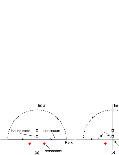
Figure 1: (Color online) The complex momentum plane. The black open squares represent the bound states and the red filled diamonds resonant states with the mirroring of the states in the imaginary axis.

Using the formalism presented above, we explore the resonances in real nuclei. By taking the nucleus ¹²⁰Sn as an example, we first perform the RMF calculation with the scalar and vector potentials being obtained. For the resonant states, the momentum representation is adopted. The Dirac equation is solved by diagonalizing the matrix (9) in the momentum space along a triangle contour, and the tip of the triangle is placed below the expected position of the resonance pole. The contour is truncated to a finite momentum $k_{\text{max}}=3.5$ fm^-1, which is sufficient for all the concerned resonances. The grid number of the Gauss-Legendre quadrature $N=120$ is used for the momentum integration along the contour, which is enough to ensure the convergence with respect to number of discretization points. In the practical calculations, the grid number $N$ is divided into $n$, $n$, and $2n$ used in each segment of the contour, respectively. For the state $h_{9/2}$, we confine the triangle contour with the four points $k=0$ fm^-1, $k=0.11-i0.008$ fm^-1, $k=0.22$ fm^-1, and $k_{\text{max}}=3.5$ fm^-1 in the complex $k$-plane. The calculated results are displayed in Fig. 2, where we can see that most solutions follow the contour, corresponding to the non-resonant continuum states. There is one solution that does not lie on the contour, corresponding to the $1h_{9/2}$ resonance, which is separated completely from the continuum and exposed clearly in the complex momentum plane.

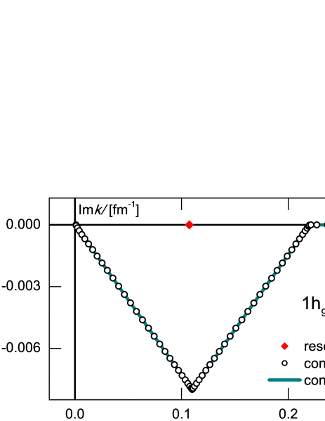
Figure 2: (Color online) Single-particle spectra for the state $h_{9/2}$ in the complex $k$-plane in the RMF-CMR calculations with the effective interaction NL3 Lal97 . The red filled diamond, black open circles, and olive solid line represent the $1h_{9/2}$ resonant state, the continuum, and the contour of integration in the complex momentum plane, respectively.

Although the resonances can be exposed in the complex $k$-plane, we would like to further check whether the present calculations depend on the choice of contour. In Fig. 3, we show the single-particle spectra for the state $f_{5/2}$ in four different contours. In each panel, one can see a resonant state exposed clearly in the complex $k$-plane. In comparison with panel (a), the contour in panel (b) is deeper, and the corresponding continuous spectra drop down with the contour, while the position of the resonant state $2f_{5/2}$ does not change. Similarly, when the contour moves from left to right or from right to left, as shown in panels (c) and (d), the continuum follows the contour, while the resonant state $2f_{5/2}$ keeps at its original position. These indicate that the physical resonant states obtained by the present method are indeed independent on the contour.

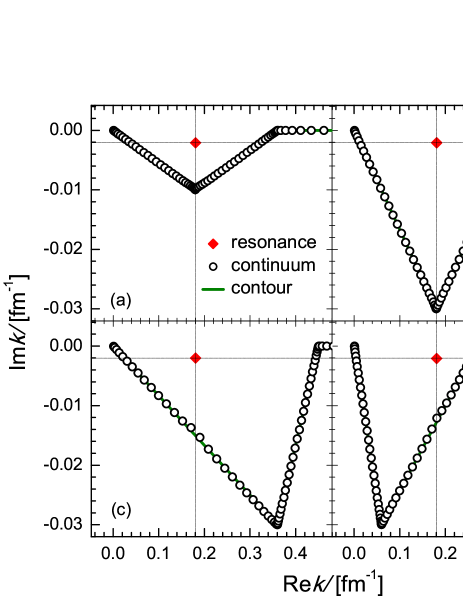
Figure 3: (Color online) Same as Fig. 2, but for the state $2f_{5/2}$ in four different contours for the momentum integration. The red filled diamond in each panel represents the $2f_{5/2}$ resonant state.

As the resonant states are independent on the contour, we can choose a large enough contour to expose all the concerned resonances. Using the one with $k=0$ fm^-1, $k=0.75-i0.28$ fm^-1, $k=1.5$ fm^-1, and $k_{\text{max}}=3.5$ fm^-1, the calculated single-neutron spectra in ¹²⁰Sn are shown in Fig. 4, where the bound states are exposed on the imaginary axis, the resonant states are isolated from the continuum in the fourth quadrant, and the continuum follows the integration contour. Here, we have observed nine resonant states $1h_{9/2}$, $2f_{5/2}$, $1i_{13/2}$, $1i_{11/2}$, $1j_{15/2}$, $1j_{13/2}$, $2g_{9/2}$, $2g_{7/2}$, and $2h_{11/2}$. For the resonant states $1h_{9/2}$, $1i_{13/2}$, and $2f_{5/2}$, their positions are close to the real $k$-axis, corresponding to the narrow resonances with smaller widths. For the resonant states $2g_{9/2}$, $2g_{7/2}$, and $2h_{11/2}$, they are far away from the real $k$-axis, corresponding to the broad resonances. Note that these broad resonances have not been obtained in the RMF-CSM calculations Guo101 because it requires a large complex rotation, which leads to the divergence of complex rotation potential. Similarly, there are also some troubles for exploring these broad resonance in other methods. The present RMF-CMR method provides a powerful and efficient pathway to explore the broad resonances as long as the momentum contour covers the range of resonance.

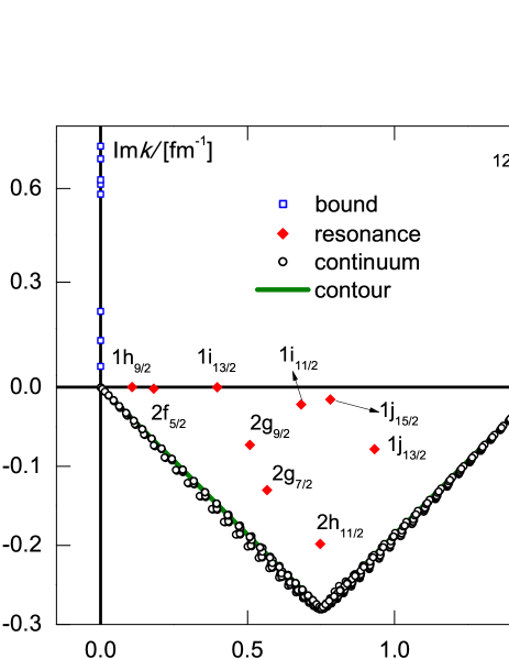
Figure 4: (Color online) Single-neutron spectra in ¹²⁰Sn in the RMF-CMR calculations with the interaction NL3. The blue open squares, red filled diamonds, and black open circles represent the bound states, the resonant states, and the continuum, respectively. The olive solid line denotes the contour of integration in the complex momentum plane.

Table 1: The calculated energies for the single neutron resonant states in ¹²⁰Sn varying with the grid number of the Gauss-Legendre quadrature in the momentum integration. More data are listed in Ref. [69]. All energies are in units of MeV.

	$1h_{9/2}$	$2f_{5/2}$	$1i_{13/2}$	$2g_{9/2}$
$N$	$E_{r}$,$E_{i}$	$E_{r}$,$E_{i}$	$E_{r}$,$E_{i}$	$E_{r}$,$E_{i}$
60	0.239,-2.81E-8	0.678,-0.0157	3.267,-0.00186	5.232,-1.534
80	0.239,-2.77E-8	0.678,-0.0156	3.267,-0.00186	5.232,-1.534
100	0.239,-2.76E-8	0.678,-0.0156	3.267,-0.00186	5.232,-1.534
120	0.239,-2.76E-8	0.678,-0.0156	3.267,-0.00186	5.232,-1.534
140	0.239,-2.76E-8	0.678,-0.0156	3.267,-0.00186	5.232,-1.534
160	0.239,-2.76E-8	0.678,-0.0156	3.267,-0.00186	5.232,-1.534

When the resonant states are exposed in the complex $k$-plane, we can read the real and imaginary parts of their wave vectors. We can then extract the resonance parameters like energy and width by the formula $E_{r}+iE_{i}=E_{r}-i\Gamma/2=\sqrt{k^{2}+M^{2}}-M$. In order to obtain precise results for the resonance parameters, it is necessary to check the convergence of the calculated results on the grid number in the Gauss-Legendre quadrature. The resonance parameters for four resonant states varying with the grid number are listed in Table 1, where three significant digits are reserved in the decimal part. From Table 1, we can see that the calculated results are unchange when $N\geqslant 80$ in the present precision with the $1h_{9/2}$ exception. For the state $1h_{9/2}$, the tiny difference among the widths should be attributed to the fact that its width is too small in comparison with the corresponding energy. These imply that we have obtained the convergent results in the present calculations.

The above discussions indicate that the present method is applicable and efficient for exploring the resonance. For comparison, the calculated results from other different bound-state-like methods, RMF-CSM Guo101 , RMF-RSM LZhang08 , and RMF-ACCC Zhang04 , are listed in Table 2 for several narrow single-neutron resonant states in ¹²⁰Sn. From Table 2, we can see that, in the RMF-CMR calculations with NL3, the energies and widths for all the available resonant states are comparable to those obtained by the other methods. The same conclusion can also be obtained in the RMF-CMR calculations with the effective interaction PK1 Long04 , which have not been shown here.

Table 2: Energies and widths of single neutron resonant states for ¹²⁰Sn in the RMF-CMR calculations in comparison with the RMF-CSM, RMF-RSM, and RMF-ACCC calculations. Data are in units of MeV.

	RMF-CMR	RMF-CSM	RMF-RSM	RMF-ACCC
$nl_{j}$	$E_{r},\Gamma$	$E_{r},\Gamma$	$E_{r},\Gamma$	$E_{r},\Gamma$
$2f_{5/2}$	0.678,0.031	0.670,0.020	0.674,0.030	0.685,0.023
$1i_{13/2}$	3.267,0.004	3.266,0.004	3.266,0.004	3.262,0.004
$1i_{11/2}$	9.607,1.219	9.597,1.212	9.559,1.205	9.60,1.11
$1j_{15/2}$	12.584,0.993	12.577,0.992	12.564,0.973	12.60,0.90

Although the agreeable results are obtained, it is worthwhile to remark the difference in these four different calculations. In the RMF-ACCC calculations, the resonant states are obtained by extending a bound state to resonant state, which is effective for the narrow resonances Zhang04 ; Guo06 ; Xu15 , but for the broad resonances the results from the ACCC calculations are less precise. Compared with the RMF-ACCC, the RMF-RSM is much simpler. The resonant states can be determined in terms of the independence of the calculated results on the model parameters. As shown in Fig. 1 in Ref. LZhang08 , there appear the plateau for the resonant states in the energy surface. For the narrow resonance $1i_{13/2}$, the plateau is clear, which implies that it is easy to determine the narrow resonances by the RMF-RSM. Although the CSM is efficient for not only narrow resonances but also broad resonances, there is the singularity in nuclear potential with a large complex rotation, which leads that the RMF-CSM is inapplicable for some broad resonances. Therefore, these four methods are all effective for the narrow resonances, while only the RMF-CMR method is applicable and more reliable for the broad resonances.

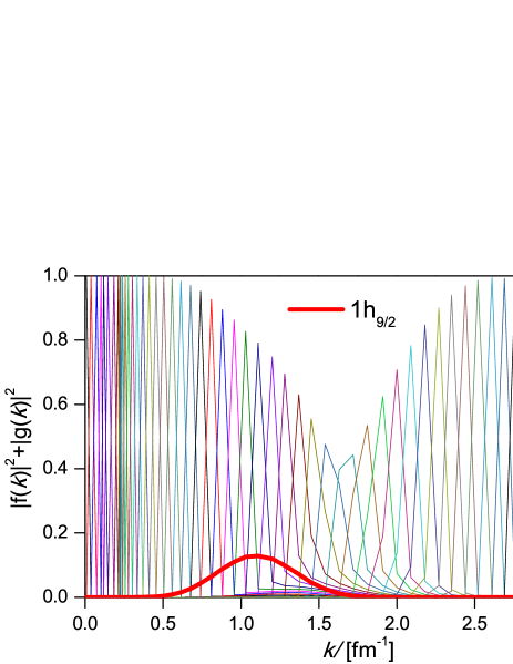
Figure 5: (Color online) Radial-momentum probability distributions for the single-particle states $h_{9/2}$. The thick red line represents the probability distributions corresponding to the $1h_{9/2}$ resonant state, while the others are the background of the continuum.

Besides the spectra, we have also obtained the wavefunction of Dirac particle in the momentum space. The radial-momentum probability distributions (RMPD) for the single-particle states $h_{9/2}$ are drawn in Fig. 5. The RMPD corresponding to the resonance $1h_{9/2}$ is expanded much wider than the surrounding states. The Heisenberg uncertainty principle tells us that a less well-defined momentum corresponds to a more well-defined position. Consequently, this state should correspond to a localized wavefunction, i.e., a wavefunction of resonant state. Compared with the $1h_{9/2}$, the RMPD for the other states display sharp peaks at different values of $k$, which correspond to free particles. These indicate that we can also judge the resonance by the wavefunction in the momentum representation.

In summary, we have proposed a new scheme to explore the resonances in the RMF framework, where the Dirac equation is solved directly in the complex momentum representation, and the bound and resonant states are dealt on an equal footing. We have presented the theoretical formalism and elaborated the numerical details. As an illustrating example, we have explored the resonances in the nucleus ¹²⁰Sn and determined the corresponding resonance parameters. In comparison with several frequently used bound-state-like methods, and the agreeable results are obtained. In particular, the present method can expose clearly the resonant states in the complex momentum plane, and determine precisely the resonance parameters without imposing unphysical parameters. Also highly remarkable is the present method is applicable for not only narrow resonances but also broad resonances that are difficult to be obtained before.

This work was partly supported by the National Natural Science Foundation of China under Grants No.11575002 and the Key Research Foundation of Education Ministry of Anhui Province under Grant No. KJ2016A026.

References

- (1) J. R. Taylor, Scattering Theory: The Quantum Theory on Nonrelativistic Collisions (John Wiley & Sons, New York, 1972).
- (2) T. Yang et al., Science 347, 60 (2015).
- (3) J. Meng and P. Ring, Phys. Rev. Lett. 77, 3963 (1996).
- (4) J. Meng and P. Ring, Phys. Rev. Lett. 80, 460 (1998).
- (5) Y. Zhang, M. Matsuo, and J. Meng, Phys. Rev. C 86, 054318 (2012).
- (6) S. G. Zhou, J. Meng, P. Ring, and E. G. Zhao, Phys. Rev. C 82, 011301 (2010).
- (7) I. Hamamoto, Phys. Rev. C 81, 021304 (2010).
- (8) A. S. Jensen, K. Riisager, D. V. Fedorov, and E. Garrido, Rev. Mod. Phys. 76, 215 (2004).
- (9) P. Curutchet, T. Vertse, and R. J. Liotta, Phys. Rev. C 39, 1020 (1989).
- (10) L. G. Cao and Z. Y. Ma, Phys. Rev. C 66, 024311 (2002).
- (11) S. S. Zhang, M. S. Smith, G. Arbanas, and R. L. Kozub, Phys. Rev. C 86, 032802(R) (2012).
- (12) T. Faestermann, P. Mohr, R. Hertenberger, and H.-F. Wirth, Phys. Rev. C 92, 052802(R) (2015).
- (13) E. P. Wigner and L. Eisenbud, Phys. Rev. 72, 29 (1947).
- (14) G. M. Hale, R. E. Brown, and N. Jarmie, Phys. Rev. Lett. 59, 763 (1987).
- (15) J. Humblet, B. W. Filippone, and S. E. Koonin, Phys. Rev. C 44, 2530 (1991).
- (16) B. N. Lu, E. G. Zhao, and S. G. Zhou, Phys. Rev. Lett. 109, 072501 (2012).
- (17) B. N. Lu, E. G. Zhao, and S. G. Zhou, Phys. Rev. C 88, 024323 (2013).
- (18) E. N. Economou, Green’s Function in Quantum Physics (Springer-Verlag, Berlin, 2006).
- (19) T. T. Sun, S. Q. Zhang, Y. Zhang, J. N. Hu, and J. Meng, Phys. Rev. C 90, 054321 (2014).
- (20) A. U. Hazi and H. S. Taylor, Phys. Rev. A 1, 1109 (1970).
- (21) V. I. Kukulin, V. M. Krasnopl’sky, and J. Horáček, Theory of Resonances: Principles and Applications (Kluwer, Dordrecht, The Netherlands, 1989).
- (22) N. Moiseyev, Phys. Rep. 302, 212 (1998).
- (23) H. S. Taylor and A. U. Hazi, Phys. Rev. A 14, 2071 (1976).
- (24) V. A. Mandelshtam, H. S. Taylor, V. Ryaboy, and N. Moiseyev, Phys. Rev. A 50, 2764 (1994).
- (25) L. Zhang, S. G. Zhou, J. Meng, and E. G. Zhao, Phys. Rev. C 77, 014312 (2008).
- (26) S. C. Yang, J. Meng, and S. G. Zhou, Chin. Phys. Lett. 18, 196 (2001).
- (27) S. S. Zhang, J. Meng, S. G. Zhou, and G. C. Hillhouse, Phys. Rev. C 70, 034308 (2004).
- (28) J. Y. Guo and X. Z. Fang, Phys. Rev. C 74, 024320 (2006).
- (29) X. D. Xu, S. S. Zhang, A. J. Signoracci, M. S. Smith, and Z. P. Li, Phys. Rev. C 92, 024324 (2015).
- (30) N. Michel, W. Nazarewicz, M. Pszajczak, and T. Vertse, J. Phys. G 36, 013101 (2009).
- (31) A. T. Kruppa, G. Papadimitriou, W. Nazarewicz, and N. Michel, Phys. Rev. C 89, 014330 (2014).
- (32) J. Carbonell, A. Deltuva, A. C. Fonseca, R. Lazauskas, Prog. Part. Nucl. Phys. 74, 55 (2014).
- (33) T. Myo, Y. Kikuchi, H. Masui, and K. Katō, Prog. Part. Nucl. Phys. 79, 1 (2014).
- (34) G. Papadimitriou and J. P. Vary, Phys. Rev. C 91, 021001(R) (2015).
- (35) J. Y. Guo, X. Z. Fang, P. Jiao, J. Wang, and B. M. Yao, Phys. Rev. C 82, 034318 (2010).
- (36) J. Y. Guo, M. Yu, J. Wang, B. M. Yao, and P. Jiao, Comput. Phys. Commun. 181, 550 (2010).
- (37) J. Y. Guo, J. Wang, B. M. Yao, and P. Jiao, Int. J. Mod. Phys. E 19, 1357 (2010).
- (38) M. Shi, J. Y. Guo, Q. Liu, Z. M. Niu, and T. H. Heng, Phys. Rev. C 92, 054313 (2015).
- (39) M. Shi, Q. Liu, Z. M. Niu, and J. Y. Guo, Phys. Rev. C 90, 034319 (2014).
- (40) C. V. Sukumar, J. Phys. A 12, 1715 (1979).
- (41) Y. R. Kwon and F. Tabakin, Phys. Rev. 18, 932 (1978).
- (42) T. Berggren, Nucl. Phys. A 109, 265 (1968).
- (43) G. Hagen and J. S. Vaagen, Phys. Rev. C 73, 034321 (2006).
- (44) A. Deltuva, Few-Body Syst. 56, 897 (2015).
- (45) R.J. Liotta, E. Maglione, N. Sandulescu, T. Vertse, Phys. Lett. B 367, 1 (1996).
- (46) N. Michel, W. Nazarewicz, M. Ploszajczak, and K. Bennaceur Phys. Rev. Lett. 89, 042502 (2002).
- (47) M. Shah, B. Pate, P. C. Vinodkumar, Eur. Phys. J. C 76, 36 (2016).
- (48) X.-N. Zhou, X.-L. Du, K. Yang, and Y.-X. Liu, Phys. Rev. D 89, 043006 (2014).
- (49) P. Stefańska, Phys. Rev. A 93, 022504 (2016).
- (50) C. Schulz, R. L. Heinisch, and H. Fehske, Phys. Rev. B 91, 045130 (2015).
- (51) J. Grineviciute and D. Halderson, Phys. Rev. C 85, 054617 (2012).
- (52) M. G. Fuda, Phys. Rev. C 64, 027001 (2001).
- (53) P. Horodecki, Phys. Rev. A 62, 052716 (2000).
- (54) B. Serot and J. D. Walecka, Adv. Nucl. Phys. 16, 1 (1986).
- (55) P. Ring, Prog. Part. Nucl. Phys. 37, 193 (1996).
- (56) D. Vretenar, A. V. Afanasjev, G. A. Lalazissis, and P. Ring, Phys. Rep. 409, 101 (2005).
- (57) J. Meng, H. Toki, S. G. Zhou, S. Q. Zhang, W. H. Long, and L. S. Geng, Prog. Part. Nucl. Phys. 57, 470 (2006).
- (58) T. Nikšić, D. Vretenar, P. Ring, Prog. Part. Nucl. Phys. 66, 519 (2011).
- (59) H. Z. Liang, J. Meng, and S. G. Zhou, Phys. Rep. 570, 1 (2015).
- (60) J. Meng and S. G. Zhou, J. Phys. G: Nucl. Part. Phys. 42, 093101 (2015).
- (61) B. Sun, F. Montes, L. S. Geng, H. Geissel, Yu. A. Litvinov, and J. Meng, Phys. Rev. C 78, 025806 (2008).
- (62) Z. M. Niu, B. Sun, and J. Meng, Phys. Rev. C 80, 065806 (2009).
- (63) J. Meng, Z. M. Niu, H. Z. Liang, and B. H. Sun, Sci. China Phys. Mech. Astron. 54(Suppl.1), s119 (2011).
- (64) X. D. Xu, B. Sun, Z. M. Niu, Z. Li, Y.-Z. Qian, and J. Meng, Phys. Rev. C 87, 015805 (2013).
- (65) Z. M. Niu, Y. F. Niu, H. Z. Liang, W. H. Long, T. Nikšić, D. Vretenar, and J. Meng, Phys. Lett. B 723, 172 (2013).
- (66) Z. M. Niu, Y. F. Niu, Q. Liu, H. Z. Liang, and J. Y. Guo, Phys. Rev. C 87, 051303(R) (2013).
- (67) G. A. Lalazissis, J.Konig, and P. Ring, Phys. Rev. C 55, 540 (1997).
- (68) W. Long, J. Meng, N. VanGiai, and S.-G. Zhou, Phys. Rev. C 69, 034319 (2004).