Diffusion of particles in simple fluids: A joint theory of kinetics and hydrodynamics

Abstract

The particle diffusion in a fluid is a classical topic that dates back to more than one century ago. However, a full solution to this issue still lacks. In this work the velocity autocorrelation function and the diffusion constant are derived analytically, and the hydrodynamics effect on the particle diffusion is analyzed in detail. Unlike previous studies, the ring-collision effect is exhaustively considered in our treatment, and the hydrodynamics approach is extended to the whole time range. Large scale molecular dynamics simulations for the hard-disk fluid show that our analytical results are valid up to the density close to the crystallization point.

The particle diffusion in a fluid is a profound issue of statistics physics. A primary attack to this problem was made by Boltzmann in 1872, and a more comprehensive understanding was obtained due to Einstein’s study Einstein in 1905 to the Brownian motion. These seminal studies established the kinetics theory, which predicts that the velocity autocorrelation function (VACF) of a particle decays exponentially, implying immediately a time-independent diffusion constant theorySP ; Leener . However, it was found later by Alder and Wainwright in 1967 that the VACF may feature a long-time tail Alder , suggesting that the kinetics theory is not thorough yet. Since then the long-time tail has been intensively studied theorySP ; Leener ; Alder ; Alder2 ; Alder3 ; wain-tlnt ; Dorfman1 ; Dorfman2 ; Dorfman3 ; Ernst ; tlnt ; cv-longtail ; review-l-t-coupling ; high-density ; formula-2d ; 2d-tailnotimport ; Erpenbeck and has been attributed to the hydrodynamics effect. To harmonize these results, the diffusion process is divided into two stages, the kinetics stage (KS) for short time and the hydrodynamics stages (HS) for long time theorySP , and the VACF reads

$${C(t)}/{\Omega}=\left\{\begin{array}[]{ll}\exp({-\Omega t/D_{k}}),&\text{KS;}\\ \sim[(1-1/d)/n][4\pi(D_{k}+\nu_{k})t]^{-\frac{d}{2}},&\text{HS}.\end{array}\right.$$ (1)

Here $t$, $n$, $D_{k}$, $\nu_{k}$, and $d$ are, respectively, the correlation time, average particle number density, kinetics diffusion constant, kinetics viscosity diffusivity, and dimensionality of the system; ${\Omega=C(0)=k_{B}T/m}$ ($k_{B}$ and $T$ are the Boltzmann constant and the system temperature; $m$ is the mass of particles). The hydrodynamics consideration provides a correction to Einstein’s picture, and as a result, the diffusion constant, denoted by $D(t)$, turns out to be time dependent following the Green-Kubo formula  theorySP ; Kubo ; Andrieux ; In particular, the correction to the diffusion constant is finite for $d=3$ but makes the diffusion constant divergent in the thermodynamical limit for $d=2$.

Despite of these developments, how a particle diffuses in a fluid is still unclear. On one hand, qualitatively, the tail of the VACF may not follow the predicted power law. For example, for $d=2$, it has been shown that the asymptotic self-consistent solution of the VACF is $C(t)\sim(t\sqrt{\ln t})^{-1}$ instead wain-tlnt ; tlnt . In a recent careful numerical study of the hard-disk fluid, it has been found that the VACF tends to $\sim t^{-1}$ at low densities but $\sim(t\sqrt{\ln t})^{-1}$ at moderate densities pre2008 . On the other hand, quantitatively, the amplitude of the power-law tail given by the hydrodynamics theory suffers from a cut-off approximation in the wave-vector space theorySP ; in addition, the transition time from the KS to the HS has not been identified precisely either. All these limitations make it impossible to accurately evaluate the hydrodynamics effect based on the existing theory.

In clear contrast, the experimental techniques have been developed so fast in recent years that nowadays it has been possible to measure the instantaneous velocity of a Brownian particle in laboratories Science ; Nature ; WangBo . More importantly, the hints of the hydrodynamics effect have been evidenced Nature . It is thus highly desired to give the particle diffusion process a thorough theroy. Motivated by this, in the present work we derive the VACF and the diffusion constant by an accurate analytical study. First of all, the ring-collision effect is taken into full consideration to calculate the hydrodynamics contribution by means of the linearizing hydrodynamics approach. We then combine the kinetics contribution to get two coupled equations for both the VACF and the diffusion constant and to get their explicit solutions. Finally, the obtained analytic results are carefully scrutinized with large scale molecular dynamics simulations of the two-dimensional hard-disk fluid.

The key point of our consideration is that the kinetics and hydrodynamics processes take place simultaneously. Without loss of generality, we suppose that initially a tagged particle resides at the origin and moves along the $x$ axis with the momentum $p_{x}^{c}=mu_{x}^{c}$, where $u_{x}^{c}$ is its initial velocity. $p_{x}^{c}$ also represents the memory of the particle’s initial moving direction. As the system evolves, upon the collisions between the tagged particle and other particles, $p_{x}^{c}$ will transfer to the latter. We refer to this process, i.e., the initial momentum of the tagged particle transferring away from it, as the kinetic process, and denote the portion of $p_{x}^{c}$ that has not transferred at time $t$ as $p_{x}^{k}(t)$. On the other hand, it is possible for the portion of $p_{x}^{c}$ that has transferred away to transfer back to the tagged particle via ring collisions Alder2 . Such a feedback is a collective effect of the surrounding particles which we refer to as the hydrodynamic process and denote the portion of $p_{x}^{c}$ that returns back to the tagged particle at time $t$ as $p_{x}^{h}(t)$. Following the definition of the VACF, $C(t)=\langle u_{x}(t)u_{x}^{c}\rangle=\langle p_{x}(t)p_{x}^{c}\rangle/m^{2}$, the VACF as well as the diffusion constant can be divided into two parts respectively, i.e., $C(t)=C_{k}(t)+C_{h}(t)$ and $D(t)=D_{k}(t)+D_{h}(t)$.

We assume that $C_{k}(t)$ follows the kinetics prediction, i.e., $C_{k}(t)={\Omega}\exp({-\Omega t/D_{k}})$ Dorfman2 ; Dorfman3 . To obtain $C_{h}(t)$ and $D_{h}(t)$, we calculate $p_{x}^{h}(t)$ in the following. Let $p(\mathbf{r},t)$ represent the density of the initial momentum transferring to the unit volume at position $\mathbf{r}$ and time $t$ and the probability with which the tagged particle appears in this area is $\rho(\mathbf{r},t)$; then on average the portion of the initial momentum returns to the tagged particle is $\rho(\mathbf{r},t)p(\mathbf{r},t)/n$. The total amount of the initial momentum returns to it is thus

$$p_{x}^{h}(t)=(1/n)\int p(\mathbf{r},t)\rho(\mathbf{r},t)d\mathbf{r}.$$ (2)

In this way, the ring-collision effect of various orders is integrated exhaustively.

We calculate $p(\mathbf{r},t)$ by hydrodynamics approaches. With the conventional assumption that the mean velocity of the fluid is zero and the local deviations of a hydrodynamic variable from its average value are small, we get $\mathbf{p}(\mathbf{r},t)=mn\mathbf{u}(\mathbf{r},t)=m\mathbf{j}(\mathbf{r},t)$, where $\mathbf{j}(\mathbf{r},t)$ is the local particle current. The relaxation properties of the momentum is thus connected to the particle current. We then have the conservation equations of the total particle number, the energy, and hte momentum of the system under this assumption, and by linearizing them with the help of the double transforms with respect to space (Fourier) and time (Laplace), we get the hydrodynamics equations (see, e.g., Ref. theorySP ). This is conventional in the hydrodynamics approaches, but our particular treatment SM is to solve the equations with the specific initial conditions of $[p_{x}(0,0),p_{y}(0,0),p_{z}(0,0)]$ $=[p_{x}^{c}\delta(\mathbf{r}),0,0]$, $\Delta T(0,0)=\Delta T\delta(\mathbf{r})$, and $\Delta n(0,0)=\Delta n\delta(\mathbf{r})$ for a three dimensional fluid, which gives the heat mode

$$\frac{p^{heat}(\mathbf{k},t)}{p_{x}^{c}}=\frac{k_{y}^{2}+k_{z}^{2}}{k^{2}}\exp(-\nu_{k}k^{2}t)$$ (3)

and the sound mode

$$\frac{p^{sound}(\mathbf{k},t)}{p_{x}^{c}}=\frac{k_{x}^{2}}{k^{2}}\exp(-\Gamma k^{2}t)\cos(c_{s}kt)$$ (4)

of the momentum (or particle current) fluctuation under the long wave approximation (up to the $\sim k^{2}$ term). Here $c_{s}$ is the sound speed and the parameter $\Gamma$ represents the sound attenuation coefficient defined in Ref. theorySP , p. 229. We then get $p(\mathbf{k},t)=p^{heat}(\mathbf{k},t)+p^{sound}(\mathbf{k},t)$. These solutions apply to a two dimensional fluid as well with $k_{z}=0$.

As to $\rho(\mathbf{r},t)$, the kinetics theory gives $\rho(\mathbf{r},t)=\frac{1}{4\pi D_{k}t}\exp({-\frac{r^{2}}{4D_{k}t}})$. Considering that the hydrodynamics effect enhances the diffusion due to the returning of the initial momentum, we assume that $\rho(\mathbf{r},t)$ generally has the same form as given by the kinetics theory but with a time-dependent diffusion constant $D_{h}(t)+D_{k}$ instead. Transforming it with respect to the space, we get $\rho(\mathbf{k},t)=\exp[-(D(t)+D_{k})k^{2}t]$.

To find the solution of Eq. (2) we employ the Parseval’s formula $\int_{-\infty}^{\infty}p(\mathbf{r},t)\rho(\mathbf{r},t)d\mathbf{r}=(\frac{1}{2\pi})^{2}\int_{-\infty}^{\infty}p(\mathbf{k},t)\rho(\mathbf{k},t)d\mathbf{k}$ (see e.g., Ref Rudin , p. 187) to convert the intergal in the configuration space to that in the wave-vector space, which gives

$$C_{h}(t)=\frac{\Omega(d-1)}{nd}[4\pi(D_{h}(t)+D_{k}+\nu_{k})t]^{-\frac{d}{2}}.$$ (5)

Note that in deriving this result the sound mode is neglected as its contribution is a high order small quantity SM . Eq. (5) will be the same as that given by the conventional approaches theorySP ; Dorfman1 ; Dorfman2 if one sets $D_{h}(t)=0$, but there it is an approximation result under the cut-off assumption (see e.g., Ref. theorySP , p. 248).

In deriving Eq. (5), the underlying assumption is that the initial momentum $p_{x}^{c}$ of the tagged particle has transferred to the surrounding particles completely. At short times, the portion of $p_{x}^{c}$ that the hydrodynamics process accounts for is $p_{x}^{c}[1-\exp(-{\Omega t/}D^{k})]$; the remaining portion is still carried by the tagged particle. For this reason Eq. (5) can be extended straightforwardly to the short time regime as

$$C_{h}(t)=\frac{\Omega(d-1)}{nd}(1-e^{-\frac{{\Omega}t}{D_{k}}})[4\pi(D_{h}(t)+D_{k}+\nu_{k})t]^{-\frac{d}{2}}.$$ (6)

This extended formula therefore applies to the whole time range. Inserting $C_{h}(t)$ into the Green-Kubo formula and solving the coupled equations, we get

$$C_{h}(t) = \frac{\Omega(d-1)}{nd}(1-e^{-\frac{{\Omega}t}{D_{k}}})(4\pi t)^{-\frac{d}{2}}A(t)^{-\frac{d}{d+2}}$$ (7)

$$D_{h}(t) = A(t)^{\frac{2}{d+2}}-(D_{k}+\nu_{k})$$ (8)

with $A(t)=(D_{k}+v_{k})^{2}+[G+\log(t/D_{k})-ei(-{\Omega}t/D_{k})]{\Omega}/(4\pi n)$ for $d=2$ and $A(t)=(D_{k}+\nu_{k})^{\frac{5}{2}}+(5/12{\ \pi}n)D_{k}^{-1/2}\Omega^{2/3}erf[({\Omega t}/D_{k})^{1/2}]-(5/12n)\Omega\pi^{-3/2}[1-\exp(-\Omega t/D_{k})]t^{-1/2}$ for $d=3$. Here $G=0.577...$ is the Euler-Gamma constant, $erf$ and $ei$ are respectively the error function and the exponential integral function.

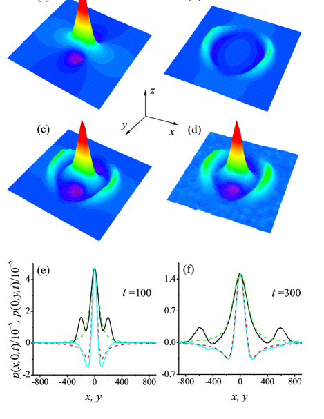
Figure 1: The analytical result of the heat mode (a), the sound mode (b), and their superposition (c) at $t=300$ for $\nu_{k}=7.7$. (d) The simulated $p(\mathbf{r},t)$ at $t=300$; (e)-(f) The intersections of the simulated $p(\mathbf{r},t)$ with $x=0$ (black solid lines) and $y=0$ (cyan solid lines) at $t=100$ and $300$, respectively. They are compared with the heat mode given by Eq. (9) with the best fitting value of $\nu_{k}=8.3$ whose intersections with $x=0$ ($y=0$) are indicated by the green dashed (red dashed) lines. For simulations $\sigma=4$.

For $d=2$, the hydrodynamics contribution of $D_{h}(t)$ diverges in the thermodynamical limit. The asymptotic solutions of Eq. (7)-(8) are $C(t)={\Omega}\sqrt{1/16\pi n}(t\sqrt{\ln t})^{-1}$ and $D(t)=\sqrt{\ln t/(4\pi n\Omega)}$, which agree with previous results wain-tlnt ; tlnt . From Eq. (6) one can further deduce that these solutions apply beyond the time scale of $t>t_{self}=\exp[(4\pi n/\Omega)(D_{k}+\nu_{k})^{2}]$ when $D_{k}+\nu_{k}$ can be ignored comparing to $D_{h}(t)$. For $t<t_{self}$, the VACF experiences a transition from $\sim t^{-1}$ to $\sim(t\sqrt{\ln t})^{-1}$. Particularly, in the period that $D_{h}(t)$ is negligible comparing to $D_{k}+\nu_{k}$, the tail of the VACF can be well approximated with $\sim t^{-1}$. For $d=3$, the VACF converges asymptotically to $\sim t^{-3/2}$, and $D_{h}(t)$ converges to the constant ${D_{h}(\infty)=[{\left(D_{k}+\nu_{k}\right)}^{5/2}+\frac{5}{12n{\pi}}(D_{k})^{-1/2}\Omega^{3/2}]}^{2/5}-(D_{k}+\nu_{k})$ which gives the upper bound of the hydrodynamics contribution.

In the following we put these analytical results into numerical tests with the hard-disk fluid model. This model is the simplest paradigmatic fluid model but has general importance for fluids since its structure do not differ in any significant way from that corresponding to more complicated interatomic potentials theorySP . It consists of $N$ disks of unitary mass $m=1$ moving in an $L\times L$ square box with the periodic boundary conditions. As the VACF is free from the finite-size effects for time $t<t_{f}=L/(2c_{s})$ pre2008 ; chenfinite ; SM , the box should be big enough to guarantee the computed tail of the VACF to be accurate. In our simulations the system size is fixed at $L=2000$ and $N=40000$ throughout. As such the average disk number density is fixing at $n=0.01$ and the disk diameter, $\sigma$, is adopted to control the packing density $\phi=n\pi\sigma^{2}/4$ (referred to as the density for short in the following). In particular, $\sigma=2$ to $9$ is investigated numerically that covers both the regimes of gas and liquid. As a reference, the crystallization density is $\phi=0.71$, corresponding to $\sigma=9.5$. The system is evolved with the event-driven algorithm Alder ; cal at the dimensionless temperature $T=1$ ($k_{B}$ is set to be unity).

$\sigma(\phi)$	2(0.03)	4(0.13)	6(0.28)	8(0.50)	9(0.63)
$\nu_{k}$(E)	14.1	7.7	6.3	8.5	14.3
$\nu_{k}$(S)	14.3	8.3	8.05	15.0	35.0
$c_{s}$(E)	1.51	1.85	2.72	5.50	9.97
$c_{s}$(S)	1.65	1.97.	2.81	5.71	9.85
$D_{k}$(E)	13.4	5.70	2.76	1.10	0.59
$D_{k}$(S)	13.61	5.50	2.35	0.54	0.27
$D^{h}(t)/D^{k}$	0.14	0.69	2.09	7.29	7.32

Table 1: Comparison of the kinetics coefficients for the hard-disk fluid model obtained by the Enskog formula (E) and by our analytical prediction based on the simulation results of $p(\mathbf{r},t)$ (S). $t=10^{7}$ for $D^{h}(t)$ in the last row.

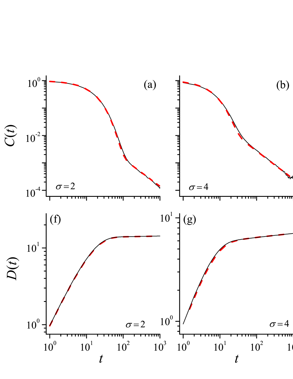
Figure 2: (Color online) (a)-(e) Comparison of the simulated VACFs (black solid lines) and the analytical results with the parameters $\nu_{k}$ and $D_{k}$ given by our computations (red dotted lines) at various system densities. (f)-(j) The same as (a)-(e) but for the diffusion constant.

We first check the prediction of the hydrodynamics modes. For the heat mode, the inverse Fourier transform of Eq. (3) with respect to space gives

$$\frac{p^{heat}(\mathbf{r},t)}{p_{x}^{c}}=\frac{x^{2}-y^{2}}{2\pi r^{4}}(1+e^{-\frac{r^{2}}{4\nu_{k}t}})+\frac{y^{2}}{4\pi r^{2}\nu_{k}t}e^{-\frac{r^{2}}{4\nu_{k}t}}.$$ (9)

Similarly, the sound mode can be obtained by the inverse transform of Eq. (4) (in form of series expansion SM ). Combining them together, we then have the analytical result of $p(\mathbf{r},t)$. An example for $\nu_{k}=7.7$ (the Enskog value for $\sigma=4$) is given in Fig. 1(a)-(c). Noting that $p(\mathbf{r},t)$ is not isotopic. Numerically, it is computed by the spatiotemporal correlation function $\langle\widetilde{p}(\mathbf{r},t)p_{x}^{c}\rangle$  chendiffusion :

$$\frac{p(\mathbf{r},t)}{p_{x}^{c}}=\frac{\langle\widetilde{p}(\mathbf{r},t)p_{x}^{c}\rangle}{\langle|p_{x}^{c}|^{2}\rangle}+\frac{n}{N-1}.$$ (10)

Here $\widetilde{p}(\mathbf{r},t)$ represents the temporal momentem density. See Fig. 1(d) for the simulated $p(\mathbf{r},t)$ for $\sigma=4$ as an example.

The explicit expression of the heat mode allow us to compute the viscosity diffusivity $\nu_{k}$ numerically based on our equilibrium simulations of $p(\mathbf{r},t)$. This can be done conveniently by best fitting the heat mode, i.e, the center peak, of the simulated $p(\mathbf{r},t)$ [see Fig. 1(d)] with $p^{heat}(\mathbf{r},t)$. In this way, we find that the $\nu_{k}$ value for the illustrating case of $\sigma=4$ is $\nu_{k}=8.3$. Note that this ‘measurement’ does not depend on time [see Fig. 1(e)-(f) for two different times], implying that the viscosity diffusivity is not affected by the hydrodynamics effect. In fact, previous numerical studies using the Helfand-Einstein formula have shown that it does not depend on the system size either formula-2d ; 2d-tailnotimport , which also supports that the viscosity diffusivity is a time-independent constant. Table I summarizes the value of $\nu_{k}$ computed in this way for various system densities and the sound speed computed by tracing the sound mode (i.e., side peaks) of the simulated $p(\mathbf{r},t)$. It is important to notice that the $\nu_{k}$ value we obtain agrees very well with that given by the Enskog formula (under the first Sonine polynomial approximation formula-2d ; Gass ; pl-eskog ) at the dilute gas regime but deviates remarkably as the density increases. In contrast, the sound speed values agrees with each other very well for all the densities.

To compare the simulated $p(\mathbf{r},t)$ with the analytical prediction, we assume the numerically measured value of $\nu_{k}$ in the latter and find the agreement is perfect in both the gas and liquid regimes even in a very dense liquid case ($\sigma=8$). But as expected, if the Enskog value of $\nu_{k}$ is taken, then the agreement is perfect only in the dilute gas case. For a moderate density the agreement can be good qualitatively with noticeable difference [compare Fig. 1(c) and (d)].

Next we turn to the instantaneous diffusion constant. Numerically it can be computed by the Green-Kubo formula, $D(t)=\int_{0}^{t}C(t^{\prime})dt^{\prime}$, if $C(t)$ is calculated. It can also be calculated according to its definition, $D(t)=d\langle r^{2}(t)\rangle/dt$, by tracing the tagged particle directly for $\langle r^{2}(t)\rangle$. The two ways give the same result SM . Figure 2(a)-(e) show the VACF at different densities, whose tail is close to $\sim t^{-1}$ but deviates differently. Taking the Enskog kinetics coefficients given in Table I, we have $t_{self}=$ $10^{23}$, $10^{10}$, $10^{4}$, $10^{13}$, and $10^{35}$ for the corresponding densities. The value of $t_{self}$ is big at the dilute and the dense limit because in the former $D_{k}$ is big and in the latter $\nu_{k}$ becomes big. In both cases $D_{h}(t)$ is comparatively small in a remarkably long time range in which it can be neglected and $C(t)\sim t^{-1}$ is expected [see Eq. (6)]

We have evidenced the considerable deviation of the computed $\nu_{k}$ from the Enskog value. For $D_{k}$ this is also the case. To evaluate $D_{k}$, we have $D(t)=D_{h}(t)+D_{k}=A(t)^{\frac{2}{d+2}}-\nu_{k}$ [see Eq. (6)], hence by taking the simulated $D(t)$ and numerically measured $\nu_{k}$ we can solve $A(t)$ and thus $D_{k}$. In doing so we have to adopt a big enough value of $t$ to make sure that the solved $D_{k}$ is a constant whose value does not change if $t$ is increased further. The $D_{k}$ value obtained in this way is presented in Table I; it can be seen that it is close to the corresponding Enskog value at low densities but deviates increasingly again as the density increases.

Applying the values of $D_{k}$ and $\nu_{k}$ measured in our method, we find that the analytical results of $C(t)$ and $D(t)$ agree perfectly with simulated ones, except an obvious disagreement in the VCAF at the highest density we have investigated ($\sigma=9$): a dip appears around the transition point $t\approx\tau$ and as a result the predicted $D(t)$ is slightly larger than the simulated result for $t>\tau$ [Fig. 2(j)]. The dip may be induced by the lattice feature as the system is close to the crystallization phase. Nevertheless, the diffusion constant can still be predicted fairly well due to the long power law tail that becomes dominant.

It is useful for application aims to have an estimation of the hydrodynamics effect in a macroscopic system. The average distance between two neighboring molecules in the air is about $10^{-9}$ meter; given that our model has a macroscopic size, say one centimeter, we have $L\sim 10^{8}$ and as such the time a particle diffuses freely without being influenced by the boundaries is $t_{f}\sim 10^{7}$. In Tab. I the ratio $D_{h}(10^{7})/D_{k}$ for the hard-disk fluid is listed, from which it can be seen that in a dilute gas the kinetics contribution dominates, but as the density increases, the hydrodynamics contribution increases dramatically and the kinetics contribution turns out to be negligible.

The hydrodynamics influence is much weaker for a three-dimensional system because of the fast convergence of the Green-Kubo integral. Adopting the kinetics coefficients of the hard-disk fluid for an estimation, we find ${D_{h}(\infty)/D^{k}<}1\%$ in general. Only in certain extreme situations, for example $D^{k}\rightarrow 0$ in the crystallization limit, the hydrodynamics contribution may become comparable to that of the kinetics.

In summary, based on the consideration that the kinetics and hydrodynamics processes take place simultaneously and by characterizing them with the losing and returning of the memory to the initial state of a particle, we have derived explicitly the VACF and the diffusion constant of a simple fluid, which are firmly corroborated by the numerical study of the hard-disk fluid model. It is found that (1) in the two-dimensional case, the hydrodynamics influence to the particle diffusion is negligible in the dilute gas regime but becomes dominant at high densities. For a three-dimensional fluid, the hydrodynamics influence is in general negligible; (2) The relaxation of momentum is not isotropic. This is different from the relaxation of mass-density fluctuations theorySP . (3) Our simulations show that the Enskog formula should be improved for calculating kinetics coefficients when the system density is high.

This work is supported by the National Natural Science Foundation of China (Grant No. 11335006) and the NSCC-I computer system of China.

References

- (1) A. Einstein, Ann. Phys. (Leipzig) 17, 549 (1905).
- (2) J. P. Hansen and I. R. McDonald, Theory of Simple Liquids, 3rd ed. (Academic, London, 2006).
- (3) P. Reusibois and M. de Leener, Classical Kinetic Theory of Fluids, Wiley-Interscience, New York, 1977.
- (4) B. S. Alder and T. E. Wainwright, Phys. Rev. Lett. 18, 988 (1967);
- (5) B. S. Alder and T. E. Wainwright, Phys. Rev. A 1,18 (1970).
- (6) B. S. Alder, D. M. Gass, and T. E. Wainwright, J. Chem. Phys. 53, 3813 (1970).
- (7) T. E. Wainwright, B.J. Alder, and D. M. Gass, Phys. Rev. A 4, 233 (1971).
- (8) S. R. Dorfman and E. G. D. Cohen, Phys. Rev. Lett. 25, 1257(1970)
- (9) J. R. Dorfman and E. G. D. Cohen, Phys. Rev. A 6, 776 (1972)
- (10) S. R. Dorfman and E. G. D. Cohen, Phys. Rev. A.12, 292 (1975).
- (11) M. H. Ernst, E. H. Hauge, and J. M. J. van Leeuwen, Phys. Rev. A 4, 2055 (1971)
- (12) D. Forster, D. R. Nelson, and M. J. Stephen, Phys. Rev. A 16 732 (1977).
- (13) J. J. Erpenbeck and W. W. Wood, Phys. Rev. A 26, 1648 (1982); Phys. Rev. A 32, 412 (1985).
- (14) Y. Pomeau and P. Reuibois, Physics Reports, 19, 63 (1975).
- (15) J. W. Dufty, Mol. Phys. 100, 2331, (2002); J. W. Dufty and M. H. Ernst, ibid, 102, 2123 (2004).
- (16) R. Garcia-Rojo, S. Luding, and J. J. Brey, Phys. Rev. E 74, 061305 (2006).
- (17) S. Viscardy and P. Gaspard, Phys. Rev. E 68, 041204 (2003).
- (18) J. J. Erpenbeck and W. W. Wood, Phys. Rev. A 26, 1648(1982)
- (19) R. Kubo, M. Toda, and N. Hashitsume, Statistical Physics II: Nonequilibrium Statistical Mechanics (Springer, New York, 1991);
- (20) D. Andrieux and P. Gaspard, J. Stat. Mech. P02006 (2007).
- (21) M. Isobe, Phys. Rev. E 77, 021201 (2008).
- (22) Tongcang Li, Simon Kheifets, David Medellin and Mark G. Raizen, Science 328, 1673 (2010).
- (23) Thomas Franosch, Matthias Grimm, Maxim Belushkin, Flavio M. Mor, Giuseppe Foffi, LazloForro and Sylvia Jeney, Nature, 478, 85 (2011).
- (24) Bo Wang, James Kuo, Sung Chul Bae and Steve Granick, Nature Materials 11, 481(2012).
- (25) Rudin, Walter (1987), Real and Complex Analysis, 3rd ed., (Singapore: McGraw Hill, 1987).
- (26) D. C. Rapaport, J. Comput. Phys. 34, 184 (1980).
- (27) D. M. Gass, J. Chem. Phys. 54, 1898 (1971).
- (28) J. J. Erpenbeck and W. W. Wood, Phys. Rev. A 43, 4254 (1991).
- (29) S. Chen, Y. Zhang, J. Wang, and H. Zhao, Phys. Rev. E 89, 022111 (2014).
- (30) S. Chen, Y. Zhang, J. Wang, and H. Zhao, J. Stat. Mech., 033205 (2016).
- (31) H. Zhao, Phys. Rev. Lett. 96, 140602 (2006).
- (32) S. Chen, Y. Zhang, J. Wang, and H. Zhao, Phys. Rev. E 87, 032153 (2013).
- (33) See the Supplimentary Material with this submission.