Blocking Collapsed Gibbs Sampler for Latent Dirichlet Allocation Models

Abstract

The latent Dirichlet allocation (LDA) model is a widely-used latent variable model in machine learning for text analysis. Inference for this model typically involves a single-site collapsed Gibbs sampling step for latent variables associated with observations. The efficiency of the sampling is critical to the success of the model in practical large scale applications. In this article, we introduce a blocking scheme to the collapsed Gibbs sampler for the LDA model which can, with a theoretical guarantee, improve chain mixing efficiency. We develop two procedures, an $O(K)$-step backward simulation and an $O(\log{K})$-step nested simulation, to directly sample the latent variables within each block. We demonstrate that the blocking scheme achieves substantial improvements in chain mixing compared to the state of the art single-site collapsed Gibbs sampler. We also show that when the number of topics is over hundreds, the nested-simulation blocking scheme can achieve a significant reduction in computation time compared to the single-site sampler.

1 Introduction

Gibbs sampling is an iterative scheme to generate random samples from a posterior distribution, which has underpinned many important applications in Bayesian statistics and machine learning (Andrieu et al., 2003). It is applicable when the joint distribution is difficult to sample from directly, but the distribution of each variable conditional on the rest, is known and is easy to simulate from. The Gibbs sampler often works in a single-site update (Geman and Geman, 1984) or data augmentation (Tanner and Wong, 1987) manner. Multiple sampling techniques may be applicable, such as collapsing and blocking, which are able to improve chain mixing (Liu et al., 1994). In this article, we propose a blocking scheme to improve the efficiency of the collapsed Gibbs sampler for the latent Dirichlet allocation (LDA) model, which is popular for topic modelling. We demonstrate that the proposed sampler achieves substantial improvements compared to the state of the art single-site collapsed Gibbs sampler (Griffiths and Steyvers, 2004).

The LDA model is a Bayesian hierarchical mixture model, which posits a fixed number of topics (mixture components) for a collection of documents, known as a corpus. It assumes that each document in the corpus reflects a combination of those topics. The model is then used to extract those unknown topics from a given corpus. In the model, each topic is characterised by a distinct multinomial topic-specific distribution, over a typically large vocabulary, while each document is modelled by a multinomial document-specific distribution over all topics. Thus, the distribution of the words from one document is a mixture of multinomial distributions over the vocabulary. The sharing of mixture components and the varying of mixture coefficients among documents reveals the similarity or dissimilarity of the underlying patterns of their words.

Blei et al. (2003) first proposed the LDA model to find the underlying patterns of words from corpora. Finding these patterns allows for effective corpus exploration, document classification, and information retrieval. It has multiple applications in areas such as text processing (Blei et al., 2003; Griffiths and Steyvers, 2004) and computer vision (Fei-Fei and Perona, 2005). In practical text analysis applications, LDA models have previously been fitted to corpera containing more than tens of thousands of documents, for vocabularies of over tens of thousands of unique terms and for hundreds of topics. This leads to models with many millions of parameters, which is a considerable challenge for Bayesian inference.

Many methods have been developed for inference and learning, such as variational methods (Minka and Lafferty, 2002; Blei et al., 2003; Teh et al., 2007) and the collapsed Gibbs sampling method (Griffiths and Steyvers, 2004). The collapsed Gibbs sampler generates word-topic allocations for all words in the corpus. Their conditional sampling distributions are derived by integrating out the multinomial parameters of the document-specific distributions as well as those of topic-specific ones. The topic allocation of each word is updated sequentially w.r.t. a discrete distribution over all topics, i.e. the sampler performs single-site updates. This collapsed Gibbs sampler has been shown to achieve better results faster than variational methods on small to medium corpora (Griffiths and Steyvers, 2004; Teh et al., 2007; Asuncion et al., 2009). Beyond Gibbs sampling, some researchers (Welling and Teh, 2011; Ahn et al., 2012; Patterson and Teh, 2014) have proposed using Langevin Monte Carlo methods combined with stochastic gradient techniques for posterior inference. These approaches can produce faster sampler updates, as they are only constructed from a subset of observations in each iteration. However, they have worse performance in chain mixing.

While the collapsed Gibbs sampler employs Rao–Blackwellization (Casella and Robert, 1996) to avoid explicitly sampling some parameters, it can however exhibit slow mixing because it only updates one hidden state assignment at a time (Celeux et al., 2000). As such, its performance deteriorates quickly when working with large datasets, which are typical in text analysis.

Various attempts have been made to scale up the collapsed Gibbs sampler to analyse increasingly large scale document corpora. Some researchers have proposed developing sampling strategies that can mimic the collapsed Gibbs dynamic, under distributed or online mini-batch settings (Smyth et al., 2009; Newman et al., 2009; Canini et al., 2009). These approaches can provide substantial memory and time savings, but they are not guaranteed to sample from the true posterior distribution.

In collapsed Gibbs sampling, the cost of evaluating and simulating from discrete distributions, which have the same dimension as the number of topics, consumes a major part of the overall computation time. Several authors (Porteous et al., 2008; Yao et al., 2009; Li et al., 2014; Yuan et al., 2015) have investigated different approaches to reduce such computational complexity. Their methods either exploit the sparsity of observations, and/or use multiple cheap independent Metropolis proposals (Andrieu et al., 2003) instead of the expensive full conditional sampling distributions. Though these approaches have provided some improvements to the computation time, their sampling efficiency is ultimately hindered by the mixing rate of the single-site collapsed Gibbs sampler.

In conclusion, most of the existing work on Markov chain Monte Carlo (MCMC) methods for the LDA model attempts to achieve faster operations on computation by retaining or sacrificing the chain mixing efficiency of the collapsed Gibbs sampler. In this article, we propose a non-trivial blocking scheme for the collapsed Gibbs sampler, which is theoretically guaranteed to accelerate chain mixing (Liu et al., 1994). We first provide the background of the model and discuss existing sampling approaches in Section 2. In Section 3, we introduce the blocking scheme, from which the full conditional distributions of the blocked latent variables can be directly simulated. We develop $O(K)$-step backward simulation and $O(\log{K})$-step nested simulation schemes to achieve this. We examine the performance of the proposed blocking scheme for one simulated and two real world datasets in Section 4, and demonstrate that the proposed sampler can achieve substantial improvements in chain mixing, compared to the state of the art single-site collapsed Gibbs sampler. Regardless of its quadratic computational complexity in evaluating sampling densities, the nested-simulation blocking scheme can also achieve a reduction in computation time per iteration when there are more than a few hundred topics. In Section 5, we discuss some possible future research directions.

2 Background

We first provide a brief review of the LDA model and its associated Gibbs sampling approaches.

2.1 Model

The LDA model summarises a document collection by multiple topics, where each topic may potentially span multiple documents. A standard assumption is that the data are exchangeable, i.e. the order of documents in a collection does not matter, and that the order of words in a document does not matter.

Let $w_{dn}\in\{1,\ldots,V\}$ be the word at position $n$ in document $d$, with its value indicating a word from a vocabulary of size $V$. Document $d$ of length $N_{d}$ is then constructed as $w_{d}=(w_{d1},\ldots,w_{dN_{d}})$. Given $K$ topics, the topic-specific distribution for topic $k$ is a $V$-dimensional multinomial distribution with parameter vector $\phi_{k}=(\phi_{k1},\ldots,\phi_{kV})$, $0\leq\phi_{kv}\leq 1$ for all $v$ and $\sum_{v}\phi_{kv}=1$. That is, for topic $k$, the probability of observing $w_{dn}=v$ is $\phi_{kv}$.

Similarly, let $z_{dn}\in\{1,\ldots,K\}$ be the latent variable for each word $w_{dn}$. Its value denotes the topic to which the associated word $w_{dn}$ belongs. The value of $z_{dn}$ follows the document-specific distribution for document $d$, which is a multinomial distribution with parameter vector $\theta_{d}=(\theta_{d1},\ldots,\theta_{dK})$, $0\leq\theta_{dk}\leq 1$ for all $k$ and $\sum_{k}\theta_{dk}=1$. In document $d$, the probability that $z_{dn}=k$, i.e. the probability that $w_{dn}$ is associated with topic $k$, is $\theta_{dk}$.

Let $\phi_{1:K}=(\phi_{1},\ldots,\phi_{K})$ be the multinomial parameters of the topic-specific distributions for all $K$ topics and $z_{d}=(z_{d1},\ldots,z_{dN_{d}})$ be the labels for all words in document $d$. In the LDA model, the likelihood function for $w_{d}$ is a mixture of $K$ components, which are the topic-specific distributions, with mixture coefficients $\theta_{d}$. This mixture structure formation leads to a latent variable model, with the complete likelihood function

$$p(w_{d},z_{d}|\theta_{d},\phi_{1:K})=\prod_{n}\theta_{d,z_{dn}}\phi_{z_{dn},w_{dn}}.$$ (1)

If there are $D$ documents, then their words are $w_{1:D}=(w_{1},\ldots,w_{D})$ and their associated topics are $z_{1:D}=(z_{1},\ldots,z_{D})$. Let $\theta_{1:D}=(\theta_{1},\ldots,\theta_{D})$ be the multinomial parameters of the document-specific distributions for all $D$ documents. To proceed with Bayesian inference, we specify the Dirichlet distribution $\pi(\theta_{d}|\alpha_{1:K})$, with $\alpha_{1:K}=(\alpha_{1},\ldots,\alpha_{K}),\,\alpha_{k}>0$ for all $k$, as the prior for $\theta_{d}$, and the symmetric Dirichlet distribution $\pi(\phi_{k}|\beta),\,\beta>0$ as the prior for $\phi_{k}$. The posterior distribution can then be obtain from (1) as

$$\pi(z_{1:D},\theta_{1:D},\phi_{1:K}|w_{1:D},\alpha_{1:K},\beta)\propto\prod_{d}\prod_{k}\theta_{dk}^{S_{d\cdot k}+\alpha_{k}-1}\times\prod_{k}\prod_{v}\phi_{kv}^{S_{\cdot vk}+\beta-1},$$ (2)

where $S_{d\cdot k}$ is the number of words in document $d$ associated with topic $k$ and $S_{\cdot vk}$ is the number of words in all documents taking the value $v$ and being associated with topic $k$. Both $S_{d\cdot k}$ and $S_{\cdot vk}$ are functions of $w_{1:D}$ and $z_{1:D}$.

2.2 Gibbs sampling

Due to the latent variable structure (2), a data augmentation scheme, under which the sampler targets both latent variables $z_{1:D}$ and parameters $(\theta_{1:D},\phi_{1:K})$, can be naturally devised, by alternating simulation between Dirichlet densities and discrete densities as follows:

$$\theta_{d}|z_{d}\sim\prod_{k}\theta_{dk}^{S_{d\cdot k}+\alpha_{k}-1}\text{ for all }d \phi_{k}|z_{1:D}\sim\prod_{v}\phi_{kv}^{S_{\cdot vk}+\beta-1}\text{ for all }k;$$ and (3)

$$z_{dn}=k|\theta_{d},\phi_{1:K}\sim\frac{\theta_{dk}\phi_{k,w_{dn}}}{\sum_{l}\theta_{dl}\phi_{l,w_{dn}}} \text{for all }(d,n).$$

As an alternative, Griffiths and Steyvers (2004) proposed to use a collapsed Gibbs sampling scheme, in which the sampler explores the marginal posterior distribution of the latent variables $z_{1:D}$, given by

$$p(z_{1:D}|w_{1:D},\alpha_{1:K},\beta)\propto\frac{\prod_{d}\prod_{k}\Gamma(S_{d\cdot k}+\alpha_{k})\times\prod_{k}\prod_{v}\Gamma(S_{\cdot vk}+\beta)}{\prod_{k}\Gamma(S_{\cdot\cdot k}+V\beta)},$$ (4)

where $S_{\cdot\cdot k}=\sum_{v}S_{\cdot vk}$ is the number of words associated with topic $k$ in all documents. This statistic is also a function of $w_{1:D}$ and $z_{1:D}$.

We denote $z_{1:D}^{(-dn)}$ to mean $z_{1:D}$, but excluding the single element $z_{dn}$, with an analogous definition for $w_{1:D}^{(-dn)}$. The single-site collapsed Gibbs sampling approach of Griffiths and Steyvers (2004) updates each $z_{dn}$ sequentially, conditional on the remaining latent variables, from a $K$-dimensional discrete distribution

$$p(z_{dn}=k|z_{1:D}^{(-dn)},w_{1:D},\alpha_{1:K},\beta)\propto\frac{(S_{d\cdot k}^{(-dn)}+\alpha_{k})(S_{\cdot vk}^{(-dn)}+\beta)}{S_{\cdot\cdot k}^{(-dn)}+V\beta},$$ (5)

where $S_{d\cdot k}^{(-dn)}$, $S_{\cdot vk}^{(-dn)}$ and $S_{\cdot\cdot k}^{(-dn)}$, respectively, denote the values of $S_{d\cdot k}$, $S_{\cdot vk}$ and $S_{\cdot\cdot k}$ constructed from $w_{1:D}^{(-dn)}$ and $z_{1:D}^{(-dn)}$. Newman et al. (2009) show empirically that this collapsing scheme is more efficient than the data augmentation sampler (3) in achieving better predictive performance.

Although this single-site sampler is straightforward and easily to implement, it can, however, be slow to converge and mix poorly, especially for models with mixture structures. Celeux et al. (2000) attributed this mixing problem to the incremental nature of the single-site Gibbs sampler, which is unable to simultaneously move a group of variables to a different mixture component. A sampling scheme which allows a group of latent variables to be updated simultaneously may remedy this problem, as Liu et al. (1994) have proven that grouping dependent variables can improve chain mixing efficiency. Therefore, a blocking scheme within the collapsed Gibbs sampler should potentially provide a considerable performance boost.

3 Blocking

In this section, we propose a blocking scheme for the existing collapsed (5) for the LDA model, which can improve chain mixing with a theoretical guarantee. We first construct the sufficient statistic w.r.t. $\theta_{1:D}$ and $\phi_{1:K}$, which naturally leads to a blocking scheme. We then develop a backward simulation and a nested simulation for exact sampling from the full conditional distributions of the blocked latent variables.

3.1 Sufficient statistic

For document $d$, we define $n_{dvk}=\sum_{n}\delta_{(v,k)}(w_{dn},z_{dn})$ to be a statistic of $(w_{d},z_{d})$, where $\delta_{(v,k)}(w_{dn},z_{dn})=1$ if and only if $(w_{dn},z_{dn})=(v,k)$. Hence, $n_{dvk}$ enumerates the number of times word $v$ is associated with topic $k$ in document $d$. In this way, we can summarise $(w_{d},z_{d})$ by a $V\times K$ matrix $\mathbb{N}_{d}$ with entries $n_{dvk}$.

In the following, we show that $\mathbb{N}_{d}$ is sufficient for $(\theta_{d},\phi_{1:K})$ in the complete likelihood function (1). Let $n_{d\cdot k}=\sum_{v}n_{dvk}$ be the number of $z_{dn}$ being equal to $k$, and $n_{dv\cdot}=\sum_{k}n_{dvk}$ be the number of times word $v$ appears in document $d$. Define $C_{dv}=\sum_{n}\sum_{k}\delta_{(v,k)}(w_{dn},z_{dn})$ to be the total count of word $v$ in document $d$. Grouping those terms $\theta_{d,z_{dn}}\phi_{z_{dn},w_{dn}}$ for which $(w_{dn},z_{dn})$ takes the same values $(v,k)$, we can rewrite the complete likelihood function (1) as

$$p(w_{d},\mathbb{N}_{d}|\theta_{d},\phi_{1:K})=\prod_{v}\left\{\frac{C_{dv}!}{\prod_{k}(n_{dvk}!)}\times\prod_{k}(\theta_{dk}\phi_{kv})^{n_{dvk}}\right\},$$ (6)

where $\prod_{v}\frac{C_{dv}!}{\prod_{k}(n_{dvk}!)}$ is the total number of equivalent realisations of $z_{d}$, i.e. those realisations of $z_{d}$ leading to the same $\mathbb{N}_{d}$ given $w_{d}$. Note that (6) is equal to (1) up to a multiplicative constant. Therefore, $\mathbb{N}_{d}$ is sufficient for $\theta_{d}$ and $\phi_{1:K}$.

For all $D$ documents, the corresponding 3-dimensional matrix of sufficient statistic is $\mathbb{N}_{1:D}=(\mathbb{N}_{1},\ldots,\mathbb{N}_{D})$. Given the Dirichlet priors for each $\theta_{d}$ and $\phi_{k}$, the collapsed posterior (4) can be derived by integrating out $\theta_{1:D}$ and $\phi_{1:K}$, which gives

$$p(\mathbb{N}_{1:D}|w_{1:D},\alpha_{1:K},\beta)\propto\frac{\prod_{d}\prod_{k}\Gamma(n_{d\cdot k}+\alpha_{k})\times\prod_{k}\prod_{v}\Gamma(n_{\cdot vk}+\beta)}{\prod_{d}\prod_{v}\prod_{k}(n_{dvk}!)\times\prod_{k}\Gamma(n_{\cdot\cdot k}+V\beta)}.$$ (7)

Due to the sufficiency, all equivalent realisations of $z_{d}$ given $w_{d}$ are uniformly distributed. In particular, we consider $B_{dv}=\{z_{dn};\,w_{dn}=v\}$, which is the group of $z_{dn}$ in document $d$ with their associated $w_{dn}$ taking word $v$. Given $(n_{dvk})_{1:K}=(n_{dv1},n_{dv2},\ldots,n_{dvK})$, all the equivalent realisations of $B_{dv}$ are uniformly distributed. Therefore, the blocked sampling scheme can be built upon the above posterior distribution (7) by sequentially sampling the blocks $B_{dv}$ via sampling $(n_{dvk})_{1:K}$ for all $d,\,v$.

3.2 Blocking scheme

The blocking scheme we consider is to sample all latent variables $z_{dn}$ in the group $B_{dv}$ simultaneously, conditional on the rest. To do this, their associated sufficient statistics $(n_{dvk})_{1:K}$ can first be simulated from the full conditional distribution,

$$p((n_{dvk})_{1:K}|\text{rest})\propto\prod_{k}\frac{(n_{d\cdot k}^{[-dvk]}+\alpha_{k})^{(n_{dvk})}\times(n_{\cdot vk}^{[-dvk]}+\beta)^{(n_{dvk})}}{n_{dvk}!\times(n_{\cdot\cdot k}^{[-dvk]}+V\beta)^{(n_{dvk})}},$$ (8)

where $n_{d\cdot k}^{[-dvk]}=n_{d\cdot k}-n_{dvk}$, $n_{\cdot vk}^{[-dvk]}=n_{\cdot vk}-n_{dvk}$, $n_{\cdot\cdot k}^{[-dvk]}=n_{\cdot\cdot k}-n_{dvk}$ and $x^{(n)}=\Gamma(x+n)/\Gamma(x)=x(x+1)\cdots(x+n-1)$. Next, all $z_{dn}\in B_{dv}$ are updated jointly, by uniformly choosing from all possible topic allocations resulting in the same $(n_{dvk})_{1:K}$. In practice, this last step can be skipped because knowing $(n_{dvk})_{1:K}$ is enough to proceed the subsequent computation. If the block contains more than one variable ($C_{dv}>1$), this blocking scheme is theoretically guaranteed to accelerate chain mixing efficiency (Liu et al., 1994), as all $z_{dn}\in B_{dv}$ are dependent in the collapsed posterior distribution (4).

Direct simulation from (8) requires evaluation of its normalising constant. As this unnormalised density function is the product of $K$ functions of each $n_{dvk}$, this structure allows for a sum-of-product algorithm (Bishop, 2006) for exact computation of this collection of normalising constants, and backward (Section 3.2.1) or nested (Section 3.2.2) simulations for direct sampling from the distribution (8).

To simplify notation, we rewrite the unnormalised density function (8) as $\prod_{k}q_{k}(n_{dvk})$ with

$$q_{k}(n_{dvk})=\frac{(n_{d\cdot k}^{[-dvk]}+\alpha_{k})^{(n_{dvk})}\times(n_{\cdot vk}^{[-dvk]}+\beta)^{(n_{dvk})}}{n_{dvk}!\times(n_{\cdot\cdot k}^{[-dvk]}+V\beta)^{(n_{dvk})}},$$

for $k=1,\ldots,K$. If we let

$$h_{k_{0}:k_{1}}(c)={\displaystyle\sum_{n_{dvk_{0}}+\cdots+n_{dvk_{1}}=c}}q_{k_{0}}(n_{dvk_{0}})\times\cdots\times q_{k_{1}}(n_{dvk_{1}}),$$ (9)

where $k_{0}\leq k_{1}$, then $h_{1:K}(C_{dv})$ is the normalising constant of $\prod_{k}q_{k}(n_{dvk})$, so that the full conditional distribution of $(n_{dvk})_{1:K}$ is

$$p((n_{dvk})_{1:K}|\text{rest})=\frac{\prod_{k}q_{k}(n_{dvk})}{h_{1:K}(C_{dv})}.$$

3.2.1 Backward simulation

Backward simulation works in a sequential manner. It first samples $n_{dvK}$ from its marginal distribution. Then backwards from $k=K-1,\ldots,1$, it samples $n_{dvk}$ from its conditional distribution given $n_{dvK},n_{d,v,K-1},\ldots,$ $n_{d,v,k+1}$. Provided values of the normalising constant $h_{1:k}(c)$ for any $k\leq K$ and $c\leq C_{dv}$ are available, such a sampling procedure can be naturally devised due to the factored structure of (8).

First, the number of words in topic $K$ can be directly simulated from the discrete marginal distribution

$$p(n_{dvK}=n|\text{rest})=\frac{q_{K}(n)\times h_{1:(K-1)}(C_{dv}-n)}{h_{1:K}(C_{dv})},$$

for $n=0,1,\ldots,C_{dv}$. Then progressing backwards, the number of words for topic $k=K-1,\ldots,3$, given those previously simulated for topics $k+1,\ldots,K$, can be simulated from the distribution

$$p(n_{dvk}=n|n_{d,v,k+1},\ldots,n_{dvK},\text{rest})=\frac{q_{k}(n)h_{1:(k-1)}(C_{dv}-\sum_{l=k+1}^{K}n_{dvl}-n)}{h_{1:k}(C_{dv}-\sum_{l=k+1}^{K}n_{dvl})}.$$ (10)

for $n=0,1,\ldots,C_{dv}-\sum_{l=k+1}^{K}n_{dvl}$. For the final stage $k=2$, the configuration for the first two topics, $(n_{dv1},n_{dv2})$ can be simultaneously sampled from the joint distribution

$$p(n_{dv1}=n_{1},n_{dv2}=n_{2}|n_{dv3},\ldots,n_{dvK},\text{rest})=\frac{q_{2}(n_{2})q_{1}(n_{1})}{h_{1:2}(C_{dv}-\sum_{k=3}^{K}n_{dvk})}.$$

It is trivial to see that the product of these conditional densities leads to the target density (8).

To enable backward simulation, we need to be able to compute the normalising constants $h_{1:k}(c)$ for any $k\leq K$ and $c\leq C_{dv}$. Due to its factored structure (9), a forward summation approach can be used to recursively obtain each value of $h_{1:k}(c)$.

It is trivial that $h_{1:1}(c)=q_{1}(c)$ for any $c$. The constants $h_{1:k}(c)$ with $k\geq 2$ can be sequentially computed through the forward recursive equation

$$h_{1:k}(c)=\sum_{n=0}^{c}q_{k}(n)\times h_{1:(k-1)}(c-n),$$

as each constituent term $h_{1:(k-1)}(0)$, $h_{1:(k-1)}(1)$, $\ldots,$ $h_{1:(k-1)}(c)$ will have been previously calculated.

3.2.2 Nested simulation

Backward simulation costs $O(K)$ steps of discrete sampling. As $K$ is large in practice, the blocked sampling could be painfully slow such that its gain in chain mixing is worthless. Therefore, we propose a nested simulation scheme which takes at most $O(C_{dv}\log{K})$ steps.

In nested simulation, a binary tree is used to represent a nested partition structure of all $K$ topics. The root takes all topics, with its left-child node taking those for topic 1 to topic $K_{1/2}=[(K+1)/2]$ (where $[x]$ denotes the integer part of $x$), while its right-child node takes the rest of its parent’s topics. Each child node is then taken as a parent node in turn, with its left- and right-child nodes constructed in the same manner based on splitting the topics in half between the child nodes. This procedure is repeated until a binary tree with $K$ leaves (a leaf is a node containing only one topic) is obtained, where each node is associated with at least one topic.

Let the size of each node be the number of latent variables of its associated topics. Hence, the size of the node associated with topic $k_{0}$ to topic $k_{1}$ is $\sum_{k=k_{0}}^{k_{1}}n_{dvk}$. The nested simulation starts from the root of size $C_{dv}$, which contains all topics, and simulates downwards to obtain sizes for all nodes. The first step samples the size of its left-child (which is of size $\sum_{k=1}^{K_{1/2}}n_{dvk}$) and the size of its right-child w.r.t. the discrete sampling density

$$p(\sum_{k=1}^{K_{1/2}}n_{dvk}=n,\sum_{k=K_{1/2}+1}^{K}n_{dvk}=C_{dv}-n|\text{rest})=\frac{h_{1:K_{1/2}}(n)\times h_{(K_{1/2}+1):K}(C_{dv}-n)}{h_{1:K}(C_{dv})},$$

for $n=0,1,\ldots,C_{dv}$. Then progressing downwards, sizes for child nodes can be simulated given the size of their parent node. For each parent node associated with topics $k_{0}$ to $k_{1}$ ($k_{0}<k_{1}$) with size $\sum_{k=k_{0}}^{k_{1}}n_{dvk}>0$, sizes for the children nodes are simulated from the distribution

$$p(\sum_{k=k_{0}}^{k_{1/2}}n_{dvk}=n,\sum_{k=k_{1/2}+1}^{k_{1}}n_{dvk}=c-n|\sum_{k=k_{0}}^{k_{1}}n_{dvk}=c,\text{rest})=\\ \frac{h_{k_{0}:k_{1/2}}(n)\times h_{(k_{1/2}+1):k_{1}}(c-n)}{h_{k_{0}:k_{1}}(c)},$$ (11)

for $n=0,1,\ldots,\sum_{k=k_{0}}^{k_{1}}n_{dvk}$ where $k_{1/2}=[(k_{0}+k_{1})/2]$. Zero size parent nodes can be skipped as no latent variables belong to topics associated with this node. The nested simulation stops when sizes for all leaves are sampled. For the leaf node associated with topic $k$, its size determines the value of $n_{dvk}$. It is trivial to see that the product of these conditional densities leads to the target density (8).

To enable nested simulation, we need to be able to compute the normalising constants $h_{k_{0}:k_{1}}(c)$ for the root and all parent nodes in the binary tree. Due to its factored structure (9), a upward summation approach can be used to recursively obtain each value of $h_{k_{0}:k_{1}}(c)$.

It is trivial that $h_{k:k}(c)=q_{k}(c)$ for any $k\leq K$ and $c\leq C_{dv}$. The constants $h_{k_{0}:k_{1}}$ with $k_{0}<k_{1}$ can be sequentially computed through the upward recursive equation

$$h_{k_{0}:k_{1}}(c)=\sum_{n=0}^{c}h_{k_{0}:k_{1/2}}(n)\times h_{(k_{1/2}+1):k_{1}}(c-n).$$

as each constituent term $h_{k_{0}:k_{1/2}}(\cdot)$ and $h_{(k_{1/2}+1):k_{1}}(\cdot)$ will have been previously calculated.

3.3 Computational complexity

The blocking scheme increases the computational cost of evaluating the sampling densities, as the full conditional densities of blocked latent variables (8) are more complex compared to those for single-site updates (5). To compute the sampling densities for all $z_{dn}$ in the block $B_{dv}$ of size $C_{dv}$, the required number of operations is $O(C_{dv}^{2}K)$, which is quadratic in $C_{dv}$, while it is $O(C_{dv}K)$ for the single-site collapsed Gibbs sampler. This quadratic cost is due to the calculation of normalising constants (9), which in fact is computing $C_{dv}$-length discrete convolutions. In practise, $C_{dv}$, the number of appearances of a given word in a document, is typically not large. When $K\gg C_{dv}$, the extra computational cost resulting from the blocking scheme will not be significant, as it is still linear in $K$.

Given the sampling densities, the simulation cost of the latent variables is the other contributor to the computational complexity. To update all $z_{dn}$ in block $B_{dv}$ of size $C_{dv}$, the single-site sampler requires $C_{dv}$ sequential steps sampling from a $K$-dimensional discrete distribution, with each step costing $O(K)$ operations. For the blocked sampler, the backward simulation in theory requires $K-1$ steps, however it can terminate at any step $k\leq K$ if $C_{dv}-n_{dv1}-\cdots n_{dvk}=0$. In comparison, the nested simulation requires at most $O(C_{dv}\log{K})$ steps due to the binary tree structure. Further, in each step, backward simulation and nested simulation only require $O(C_{dv}-n_{dv1}-\cdots-n_{d,v,k+1}+1)$ and $O(n_{dvk_{0}}+\cdots+n_{dvk_{1}})$ operations respectively to simulate from their conditional density (10 and 11). These sampling operations have much less complexity than sampling from $K$-dimensional discrete distributions when $C_{dv}\ll K$.

In particular when $C_{dv}=1$, i.e. word $v$ only appears once in document $d$, computational complexity of the single-site sampling scheme and the backward-simulation blocked sampling scheme are $O(K)$ , while the nested scheme has far less computational complexity. For the computational cost of evaluating the sampling densities, the required number of operations for all schemes is $O(K)$ as $1=C_{dv}=C_{dv}^{2}$. For the simulation cost, the single-site sampler uses one simulation from a $K$-dimensional discrete distribution. The backward simulation performs sequential sampling from at most $K-1$ binomial distributions, while the nested scheme performs a binary-tree-search style sampling from at most $\log{K}$ binomial distributions.

4 Experiments

The performance of the collapsed Gibbs sampler using the proposed blocking scheme was evaluated for one simulated and two real datasets. Interest is in two aspects of performance: mixing efficiency and the time taken to learn the model. Blocked collapsed Gibbs samplers (10 and 11) are first compared to the single-site collapsed Gibbs sampler (5), and to the data augmentation sampler (3) using the simulated dataset in Griffiths and Steyvers (2004). All collapsed samplers are then compared through analyses of two real datasets: the KOS blog entries from dailykos.com and the NIPS papers dataset from books.nips.cc, both of which are available for download from the UCI Machine Learning Repository (Lichman, 2013). We demonstrate that the blocking scheme can on average achieve substantial improvements in chain mixing over the state of the art single-site sampler, with moderate additional computational cost when $K$ is small. As $K$ becomes larger, the iteration speed of nested-simulation blocked scheme achieves and surpasses the performance of the single-site sampler. This indicates that our blocking scheme is particularly suitable to models with a large number of topics, $K$.

4.1 Evaluation method

We determine the mixing efficiency of a sampler via two metrics, evaluated over the realised MCMC sample path. The first one is the logarithm of the posterior probability (4): given the same number of iterations, the sampler with better mixing efficiency can reach a region with higher log posterior probability. While the log posterior probability contains an intractable normalising constant, we equivalently evaluate the unnormalised probability

$$\mathrm{log}\,q(z_{1:D}|w_{1:D},\alpha_{1:K},\beta)=\\ \sum_{d}\sum_{k}\log\Gamma(S_{d\cdot k}+\alpha_{k})+\sum_{k}\sum_{v}\log\Gamma(S_{\cdot vk}+\beta)-\sum_{k}\log\Gamma(S_{\cdot\cdot k}+V\beta),$$ (12)

which is equal to $\log\,p(z_{1:D}|w_{1:D},\alpha_{1:K},\beta)$ plus a constant term for any $z_{1:D}$. The unnormalised log posterior probability is useful for evaluating the speed that the sampler reaches the region of high posterior probability given some starting point. The faster it reaches this region, the shorter burnin period it will have. However, this metric only measures one aspect of mixing efficiency.

The second mixing efficiency metric is the perplexity (Blei et al., 2003; Wallach et al., 2009), which is the probability assigned to unseen data given some training documents. Let $w_{A}^{\star}=\{w_{d}^{\star};\,d\in A\}$, with $w_{d}^{\star}=(w_{d1}^{\star},\ldots,w_{dN_{d}^{\star}}^{\star})$, represent the collection of unseen words in the corpus in some test set $A$. The perplexity is given by

$$\text{perp}(w_{A}^{\star}|\theta_{1:D},\phi_{1:K})=\exp\left\{-\frac{\sum_{d\in A}\sum_{v}C_{dv}^{\star}\log(\sum_{k}\theta_{dk}\phi_{kv})}{\sum_{d\in A}N_{d}^{\star}}\right\},$$ (13)

where $C_{dv}^{\star}=\sum_{n}\delta_{v}(w_{dn}^{\star})$ is the total number of occurrences of the word $v$ in $w_{d}^{\star}$. A document completion approach (Wallach et al., 2009) is used to partition each document in the test set $A$ into two sets of words, $w_{d}$ and $w_{d}^{\star}$, using $w_{d}$ to estimate $\theta_{d}$, and then calculating the perplexity on $w_{d}^{\star}$. In the $l^{\text{th}}$ MCMC iteration, $\theta_{dk}$ and $\phi_{kv}$ are respectively estimated by

$$\theta_{dk}^{(l)}=\frac{S_{d\cdot k}^{(l)}+\alpha_{k}}{N_{d}+\sum_{k}\alpha_{k}}\quad\text{ and }\quad\phi_{kv}^{(l)}=\frac{S_{\cdot vk}^{(l)}+\beta}{S_{\cdot\cdot k}^{(l)}+V\beta}.$$

For every $L=10$ iterations, the sample mean $\frac{1}{L}\sum_{l}\left(\sum_{k}\theta_{dk}^{(l)}\phi_{kv}^{(l)}\right)$ is used to estimated the $\sum_{k}\theta_{dk}\phi_{kv}$ term in (13), in order to circumvent the label switching problem (Celeux et al., 2000) in MCMC samples. The perplexity can measure the ability of a sampler to explore the posterior density. The sampler which better explores this region can provide estimators with better predictive performance, and thereby a lower perplexity value.

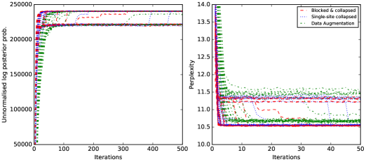
Figure 1: The unnormalised log posterior probability (left) and the perplexity (right) of the blocked collapsed Gibbs sampler (dashed), the single-site collapsed Gibbs sampler (dotted), and the data augmentation sampler (dashed & dotted) for the simulated dataset ($D=2,000,\,V=25,\,K=10$).

4.2 Results for simulated data

We analyse a simulated corpus of $D=2,000$ documents following the model setup of Griffiths and Steyvers (2004), with $K=10$ topics for all documents and $V=25$ unique words in the vocabulary. Each document in the simulated corpus has $100$ words, and the hyper-parameters in the model are set to be $\alpha_{k}=0.1$ for all $k$ and $\beta=0.01$. To evaluate the perplexity, we hold out half of the words in the last $250$ documents as the test dataset, with the remainder as training data. That is, $N_{d}=100$ for $d\leq 1,750$ and $N_{d}=N_{d}^{\star}=50$ for $d>1,750$. We implement the blocked and single-site collapsed Gibbs samplers and the data augmentation sampler 30 times, identically initialised at random points. The estimates of the unnormalised log posterior probability (12) and the perplexity (13) are shown in Figure 1.

For this small dataset, while most runs of each sampler appear to converge within $\sim 100$ iterations, not all converge to the region of the global posterior mode. Both collapsed samplers perform well on average, with relatively few runs (5 out of 30) trapped in regions of local modes after 500 iterations, compared to the data augmentation sampler (10 out of 30 runs). Both collapsed samplers consistently outperform the data augmentation algorithm in achieving lower perplexity. As the burnin efficiency of the two collapsed samplers is very rapid for most runs ($\sim 50$ iterations), the blocked sampler only achieves slightly better performance for this dataset.

While this small dataset does not demonstrate a clear advantage for the blocked collapsed Gibbs sampler over the single-site sampler, it does illustrate that sampler performance can improve even in non-challenging scenarios. However in practice, real datasets are commonly both large and sparse, such that the single-site collapsed Gibbs sampler performs poorly.

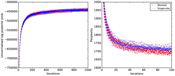
(a) KOS

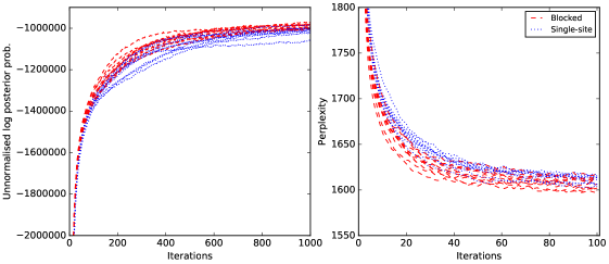
(b) NIPS

Figure 2: The unnormalised log posterior probability (left) and the perplexity (right) of the collapsed Gibbs samplers with blocking (dashed) and singe-site update (dotted) schemes for the KOS dataset with $K=32$ (top), and NIPS dataset with $K=40$ (bottom).

4.3 Results for real data

We analyse two corpora, the KOS corpus of $D=3,430$ documents with $V=6,906$ unique words and $K=32$ topics, and the NIPS corpus of $D=1,500$, $V=12,419$ and $K=40$. The KOS (NIPS) corpus has $467,714$ ($1,932,365$) total words. As before, the LDA model hyper-parameters are set to be $\alpha_{k}=0.1$ for all $k$ and $\beta=0.01$. To evaluate the perplexity, we hold out half of the words in the last 430 (250) documents of the KOS(NIPS) dataset as test data, with the remainder used as training data. We implement the blocked and single-site collapsed Gibbs samplers 20 (10) times, initialised at random points, for the KOS (NIPS) dataset. The estimates of the unnormalised log posterior probability (12) and the perplexity (13) are shown in Figure 2a (KOS) and Figure 2b (NIPS).

For the KOS dataset, the blocked sampler performs no better than the single-site sampler in terms of unnormalised log posterior probability, while it performs a little better in terms of perplexity. This is expected to occur as $62.9\%$ of words in the KOS dataset appear only once in their documents. As a result, most blocks will have only one latent variable, and so sampling such blocks is equivalent to sampling a single variable, as for the single-site collapsed Gibbs sampler. Therefore, the gain in performance achieved by blocking, while apparent, is not particularly large.

For the NIPS dataset, the performance of the blocked sampler is significantly better than the single-site sampler. The blocked sampler can reach the region of high posterior probability several hundred iterations faster than the single site sampler. Further, the blocked sampler achieves lower perplexity values on average, due to the blocking scheme which enables a more efficient exploration of the posterior density.

4.4 Time comparison results

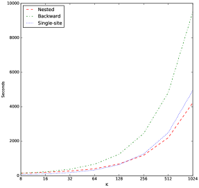
(a) KOS

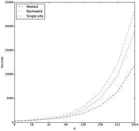
(b) NIPS

Figure 3: Average time per iteration (in seconds) for Gibbs samplers with nested blocking (dashed line), backward blocking (dashed & dotted line) and single-site update (dotted line) schemes, for KOS (left) and NIPS (right) datasets with $K$ from 8 to 1024.

To investigate the computational costs of the different collapsed Gibbs samplers, we implement blocking (nested- and backward-simulation) and single-site schemes algorithms (in Python 3.4) on the above two real datasets, replicated 10 times under different settings on a cluster node with one CPU core with the Intel Xeon E5-2670 2.60 GHz processor and 12 Gb RAM. The average time costs per iteration, measured in seconds, for each algorithm on the KOS and NIPS datasets for models with $K=8,16,\ldots,1024$ topics are shown in Figure 3.

For the smaller KOS dataset, the single-site collapsed sampler runs at more than twice the speed of the backward-simulation blocked sampler for any number of topics. For the relatively larger NIPS dataset, the backward-simulation method takes around 25% extra computation time. However, the nested-simulation blocked sampler, though only slightly better than the backward-simulation scheme when $K$ is around 16, achieves and surpasses the performance of the single-site sampler as $K$ becomes larger. In particular when $K=1024$, the nested-simulation blocked sampler can save 14.4% and 36.5% computation per iteration over the single-site sampler for the KOS and NIPS datasets, respectively. This indicates that our blocking sampler can achieve better both mixing with lower computational cost.

5 Discussion

We have introduced a novel blocking scheme for the collapsed Gibbs sampler applied to the LDA model, which can, with a theoretical guarantee, improve chain mixing (Liu et al., 1994). Our approach uses a backward simulation or nested simulation scheme to directly sample from the conditional distributions of blocked latent variables. We have demonstrated that the blocked collapsed sampler can achieve substantial improvements in chain mixing, compared to the state of the art single-site collapsed Gibbs sampler, with the nested-simulation method taking significant less computational cost for models with more than hundreds of topics.

Various directions could be explored to further reduce the computation cost for sampling each block. A more efficient simulation procedure could take topic sparsity and algorithm parallelisation into account. In addition, the $O(C^{2}_{dv})$ quadratic cost for evaluating the sampling densities can be to reduced to $O(C_{dv}\log(C_{dv}))$ by using a fast Fourier transformation based discrete convolution when $C_{dv}$ is large. It may not be possible to reduce this further to a linear cost without making an approximation. An $O(C_{dv})$ approximation to sample the block without sacrificing much efficiency is worth investigation, however.

Another research direction is to turn the proposed blocking scheme into a general methodology and extend it to other models with mixture structures. One specific possibility under investigation is to design blocking schemes for the marginal sampler of Dirichlet process mixture models (Neal, 2000) and hierarchical Dirichlet process models (Teh et al., 2006) with discrete observations and conjugate priors.

References

- Ahn et al. (2012) Ahn, S., A. Korattikara, and M. Welling (2012). Bayesian posterior sampling via stochastic gradient Fisher scoring. In Proceedings of the 29th Annual International Conference on Machine Learning, pp. 1591–1598.
- Andrieu et al. (2003) Andrieu, C., N. de Freitas, A. Doucet, and M. I. Jordan (2003). An introduction to MCMC for machine learning. Machine Learning 50(1–2), 5–43.
- Asuncion et al. (2009) Asuncion, A., M. Welling, P. Smyth, and Y. W. Teh (2009). On smoothing and inference for topic models. In Proceedings of the Twenty-Fifth Conference on Uncertainty in Artificial Intelligence, pp. 27–34.
- Bishop (2006) Bishop, C. M. (2006). Pattern Recognition and Machine Learning. New York: Springer-Verlag.
- Blei et al. (2003) Blei, D. M., A. Y. Ng, and M. I. Jordan (2003). Latent Dirichlet allocation. Journal of Machine Learning Research 3, 993–1022.
- Canini et al. (2009) Canini, K. R., L. Shi, and T. L. Griffiths (2009). Online inference of topics with latent Dirichlet allocation. In Proceedings of the Twelfth International Conference on Artificial Intelligence and Statistics.
- Casella and Robert (1996) Casella, G. and C. P. Robert (1996). Rao-Blackwellisation of sampling schemes. Biometrika 83(1), 81–94.
- Celeux et al. (2000) Celeux, G., M. Hurn, and C. P. Robert (2000). Computational and inferential difficulties with mixture posterior distributions. Journal of the American Statistical Association 95(451), 957–970.
- Fei-Fei and Perona (2005) Fei-Fei, L. and P. Perona (2005). A Bayesian hierarchical model for learning natural scene categories. In IEEE Conference on Computer Vision and Pattern Recognition, pp. 524–531.
- Geman and Geman (1984) Geman, S. and D. Geman (1984). Stochastic relaxation, Gibbs distributions, and the Bayesian restoration of images. IEEE Transactions on Pattern Analysis and Machine Intelligence 6(6), 721–741.
- Griffiths and Steyvers (2004) Griffiths, T. L. and M. Steyvers (2004). Finding scientific topics. Proceedings of the National Academy of Sciences 101(suppl 1), 5228–5235.
- Li et al. (2014) Li, A. Q., A. Ahmed, S. Ravi, and A. J. Smola (2014). Reducing the sampling complexity of topic models. In Proceedings of the 20th ACM SIGKDD international conference on Knowledge discovery and data mining.
- Lichman (2013) Lichman, M. (2013). UCI machine learning repository.
- Liu et al. (1994) Liu, J. S., W. H. Wong, and A. Kong (1994). Covariance structure of the Gibbs sampler with applications to the comparisons of estimators and augmentation schemes. Biometrika 81(1), 27–40.
- Minka and Lafferty (2002) Minka, T. and J. Lafferty (2002). Expectation-Propagation for the generative aspect model. In Proceedings of the Eighteenth Conference on Uncertainty in Artificial Intelligence, pp. 352–359.
- Neal (2000) Neal, R. M. (2000). Markov chain sampling methods for Dirichlet process mixture models. Journal of Computational and Graphical Statistics 9(2), 249–265.
- Newman et al. (2009) Newman, D., A. Asuncion, P. Smyth, and M. Welling (2009). Distributed algorithms for topic models. Journal of Machine Learning Research 10, 1801–1828.
- Patterson and Teh (2014) Patterson, S. and Y. W. Teh (2014). Stochastic gradient Riemannian Langevin dynamics on the probability simplex. In Advances in Neural Information Processing Systems 26, pp. 3102–3110.
- Porteous et al. (2008) Porteous, I., D. Newman, A. Ihler, A. Asuncion, P. Smyth, and M. Welling (2008). Fast collapsed Gibbs sampling for latent Dirichlet allocation. In Proceedings of the 14th ACM SIGKDD international conference on Knowledge discovery and data mining, pp. 569–577.
- Smyth et al. (2009) Smyth, P., M. Welling, and A. U. Asuncion (2009). Asynchronous distributed learning of topic models. In Advances in Neural Information Processing Systems 21, pp. 81–88.
- Tanner and Wong (1987) Tanner, M. A. and W. H. Wong (1987). The calculation of posterior distributions by data augmentation. Journal of the American Statistical Association 82(398), 528–540.
- Teh et al. (2006) Teh, Y. W., M. I. Jordan, M. J. Beal, and D. M. Blei (2006, 12). Hierarchical Dirichlet processes. Journal of the American Statistical Association 101(476), 1566–1581.
- Teh et al. (2007) Teh, Y. W., D. Newman, and M. Welling (2007). A collapsed variational Bayesian inference algorithm for latent Dirichlet allocation. In Advances in Neural Information Processing Systems 19, pp. 1353–1360.
- Wallach et al. (2009) Wallach, H. M., I. Murray, R. Salakhutdinov, and D. Mimno (2009). Evaluation methods for topic models. In Proceedings of the 26th Annual International Conference on Machine Learning, pp. 1105–1112.
- Welling and Teh (2011) Welling, M. and Y. W. Teh (2011). Bayesian learning via stochastic gradient Langevin dynamics. In Proceedings of the 28th Annual International Conference on Machine Learning, pp. 681–688.
- Yao et al. (2009) Yao, L., D. Mimno, and A. McCallum (2009). Efficient methods for topic model inference on streaming document collections. In Proceedings of the 15th ACM SIGKDD international conference on Knowledge discovery and data mining, pp. 937–946.
- Yuan et al. (2015) Yuan, J., F. Gao, Q. Ho, W. Dai, J. Wei, X. Zheng, E. P. Xing, T.-Y. Liu, and W.-Y. Ma (2015). LightLDA: Big topic models on modest computer clusters. In Proceedings of the 24th international conference on World wide web, pp. 1351–1361.