Investigating the Circumstellar Disk of the Be Shell Star 48 Librae

Abstract

A global disk oscillation implemented in the viscous decretion disk (VDD) model has been used to reproduce most of the observed properties of the well known Be star $\zeta$ Tau. 48 Librae shares several similarities with $\zeta$ Tau – they are both early-type Be stars, they display shell characteristics in their spectra, and they exhibit cyclic $V/R$ variations – but has some marked differences as well, such as a much denser and more extended disk, a much longer $V/R$ cycle, and the absence of the so-called triple-peak features. We aim to reproduce the photometric, polarimetric, and spectroscopic observables of 48 Librae with a self-consistent model, and to test the global oscillation scenario for this target. Our calculations are carried out with the three-dimensional NLTE radiative transfer code HDUST. We employ a rotationally deformed, gravity-darkened central star, surrounded by a disk whose unperturbed state is given by the VDD model. A two-dimensional global oscillation code is then used to calculate the disk perturbation, and superimpose it on the unperturbed disk. A very good, self-consistent fit to the time-averaged properties of the disk is obtained with the VDD. The calculated perturbation has a period $P=12$ yr, which agrees with the observed period, and the behaviour of the $V/R$ cycle is well reproduced by the perturbed model. The perturbed model improves the fit to the photometric data and reproduces some features of the observed spectroscopic data. Some suggestions to improve the synthesized spectroscopy in a future work are given.

1 Introduction

48 Librae (HD 142983, HR 5941) is a bright ($V\sim 5$) Be star that began to display shell characteristics sometime between 1931 and 1935 (Faraggiana, 1969). Its spectral features were already studied and documented extensively by the mid-1960s (see, e.g., the review by Underhill 1966), but 48 Librae has continued to be the subject of papers to the present day owing to the fact that it possesses several characteristics that make it a particularly intriguing object of study.

Be stars (sometimes referred to as Classical Be stars) are a well studied class of objects consisting of near main-sequence, rapidly rotating, B-type stars that have shown Balmer emission at some epoch. The emission lines that characterize Be star spectra have been conclusively shown to originate in a thin, equatorial disk consisting of material that has decreted from the central star. Furthermore, several recent studies have shown that these disks rotate in a Keplerian fashion (see Meilland et al. 2007; Delaa et al. 2011; Kraus et al. 2012; Wheelwright et al. 2012).

The term “shell star” is reserved for a particular subset of Be stars whose spectra display exceedingly narrow absorption cores superimposed on broad emission lines. They are understood as ordinary Be stars viewed in an edge-on configuration; this provides a very simple and natural explanation for their spectroscopic appearance, as the narrow absorption cores arise due to the large optical depths that occur when viewing the disk through its densest part. In general, shell stars are interesting objects to study because the uncertainty in their inclination angle is largely eliminated.

In addition to being a shell star, 48 Librae displays a quasi-cyclical asymmetry in its emission lines with the violet ($V$) and red ($R$) peaks of the lines usually being of unequal height, and the peak heights varying smoothly from configurations with $V>R$ to $V<R$. Known as $V/R$ variations, this behaviour is common to about one-third of all Be stars (Porter & Rivinius, 2003), although 48 Lib possesses both a very strong maximum flux and an unusually strong asymmetry in its H${\alpha}$ profile. The asymmetry can be so strong as to result in misclassifications of the star as a supergiant (i.e. the line profiles are misinterpreted as P Cyg wind profiles). An example of this can be found in the SIMBAD database where the star is still listed as B8Ia/Ib with a reference to Houk & Smith-Moore (1988).

48 Lib has long been known as a $V/R$ variable star, with the cycles in its Balmer emission lines having a period of $\sim$10 years (see, e.g., Mennickent & Vogt 1988, and the many references therein). A recent study of 48 Lib by Štefl et al. (2012) suggests that the $V/R$ variations were absent between 1995-1998, but that the cycle following that time appears to have a period of $\sim$17 years, i.e. significantly longer than previously observed. Furthermore, they found the maximum value of $V/R$ in the last cycle ($V/R\approx$ 2.2, which occurred in 2006) was greater than the maximum in the previous activity cycle. For this study, we focus solely on the most recent cycle, and therefore do not consider any data taken before 1995.

$V/R$ variations are thought to arise from a one-armed density wave precessing in the disk (Okazaki, 1997; Carciofi et al., 2009; Escolano et al., 2015). This necessarily implies that the density distribution is non-axisymmetric in the disks of stars exhibiting this phenomenon. The differing $V$ and $R$ peak heights seen in the line profiles are then explained very naturally by the changing density configurations that are seen by a stationary observer as the wave pattern precesses. The maximum value of $V/R$ observed in 48 Lib’s last cycle is larger than what is usually observed in Be stars, and suggests the density contrast in its disk may be more extreme than typical.

48 Librae appears to be an isolated star, i.e. it has no known binary companion. Therefore, its disk, which we infer to be quite dense (on average) from its large H$\alpha$ flux and strong IR excess, is very likely to be quite extended. While Be stars in binary systems may have their disk truncated at the tidal radius by the secondary star (Okazaki & Negueruela, 2001; Panoglou et al., submitted), there are no expected disk truncation mechanisms present in 48 Lib. This is considered to be somewhat of a rarity, as a large fraction of Be stars are observed to exist as binaries or multiple star systems (Sana et al., 2012).

The viscous decretion disk (VDD) model, a description of the circumstellar disk which was first introduced by Lee et al. (1991), has begun to emerge as the leading physical model of Be star circumstellar disks. In Carciofi et al. (2009), the VDD model was implemented in the radiative transfer code HDUST to reproduce the spectroscopic, polarimetric, photometric, and near-IR interferometric observations of $\zeta$ Tau. More recently, Klement et al. (2015) used the VDD model and the HDUST code in an extensive study of $\beta$ CMi. While those studies demonstrated that the VDD model could successfully reproduce most of the observables of each target, additional studies on varied targets are required to determine if the VDD model describes Be stars generally.

In this work, we use the VDD model in combination with the HDUST code, described in Carciofi & Bjorkman (2006, 2008), to investigate 48 Librae’s circumstellar disk. This represents the first attempt at applying this method to an isolated Be star with an extended disk, as both $\zeta$ Tau and $\beta$ CMi are binary stars whose disks are truncated. Furthermore, it represents only the second attempt at employing the model to reproduce cyclic $V/R$ variations. The work is organized as follows: in Sect. 2, we describe our observations, and in Sect. 3, we provide an outline of the computational codes employed, followed by a discussion of our models of the central star and the disk. In Sect. 4, we provide the results of our analysis, and in Sect. 5, we give a summary and discussion.

2 Observations

2.1 Photometry

The VO Sed Analyser (VOSA; Bayo et al. 2008) was employed to obtain photometric values spanning from the UV to the far infrared. We use International Ultraviolet Explorer (IUE) HPDP photometry for the UV portion of the SED, and Strömgren $uvby$ (Hauck & Mermilliod, 1998) and Johnson $UBV$ (Mermilliod & Mermilliod, 1994) photometry for the visible portion of the SED. Tycho-2 (Høg et al., 2000) and The Two Micron All Sky Survey (2MASS; Skrutskie et al. 2006) photometry are used for the near infrared, and The Wide-field Infrared Survey Explorer (WISE; Wright et al. 2010), The Infrared Astronomical Satellite Mission (IRAS; Helou & Walker 1988), and AKARI (Murakami et al., 2007; Ishihara et al., 2010) data are used for the far-IR portion of the SED. It should be noted that the IRAS measurements at 60$\mu$m and 100$\mu$m are upper limits only (Waters et al., 1987). Touhami et al. (2013) report a color excess $E(B-V)=0.000\pm 0.007$ for this star, and therefore no dereddening was applied. The photometric values and their respective errors are listed in Table 1.

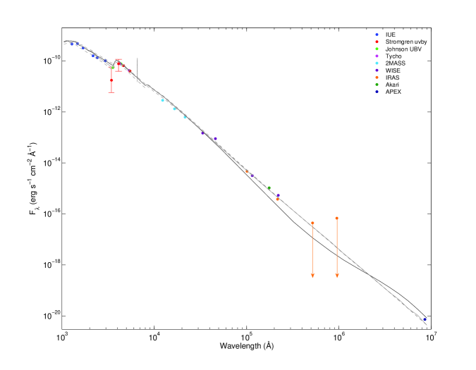
Figure 1: SED of 48 Librae. Filled circles represent measured fluxes obtained with various instruments, as indicated in the legend. The size of the points is equal to or slightly greater than the errors in the measurements, except in the two Strögrem points where error bars have been explicitly added. The two IRAS data points at 60$\mu$m and 100$\mu$m are considered upper limits only. The solid black line represents the unperturbed model created for a B3V star with an average initial disk density $\rho_{0}=8.8\times 10^{-11}$ g cm^-3 oriented at 85°. The solid grey line represents the perturbed model created with the same model star, initial density, and orientation, in a $V=R$ configuration. The dashed grey lines represent the extrema that the $V/R$ variations cause in the model SED, with the upper line representing a $V<R$ configuration and the lower line representing a $V>R$ configuration.

Clearly, the measurements used to create the SED are obtained at different epochs. As Be stars are known to be variable objects, some variation in the measurements owing to the epoch in which they were taken is therefore expected. However, strong photometric variations occur only for those Be stars whose H$\alpha$ profiles undergo phase changes from emission to absorption, which are interpreted as disk-building (emission) and disk-loss (absorption) events. 48 Lib’s H$\alpha$ profile has not been observed in absorption since it first became actively studied in the 1930s, indicating a relatively stable disk that does not dissipate. In addition, the analysis of Jones et al. (2011) indicates 48 Lib’s disk shows no clear trend of growth or loss. Moreover, in our data spanning the most recent V/R cycle, we see no systematic changes in the observed H$\alpha$ equivalent width (EW), which again indicates that the disk is not building or dissipating. For these reasons, we expect the photometry to remain fairly constant over different epochs, and anticipate only minor fluctuations in its values owing to the different configurations (due to the one-armed density oscillation) in which the disk may be viewed. This is confirmed by Figure 1, where it can be seen that the maximal change in the model caused by the different disk configurations is slight, causing the predicted fluxes to vary more or less within the error bars associated with each measurement.

2.2 Radio measurement

Radio measurements exist for only a handful of Be stars, but are extremely useful in determining the full extent of the circumstellar disk. This is because the IR and radio excesses in Be stars arise mostly from free-free emission in the ionized gas. As the free-free opacity increases with wavelength, the flux at longer wavelengths originates from progressively wider expanses of the disk (Vieira et al., 2015).

48 Lib has been detected at 870 $\mu$m by the Atacama Pathfinder EXperiment (APEX) (Güsten et al., 2006), and the data were reduced with CRUSH v. 2.31. The value of the flux is given in Table 1 along with the other photometric fluxes used in this work. The application of APEX to Be stars is described more fully in Klement et al. (2015).

2.3 Spectroscopy

High resolution H$\alpha$ profiles were collected from several sources and analyzed in order to create the observed $V/R$ cycle. A total of 49 H$\alpha$ profiles were obtained on 30 nights between 2005 and 2015 with the fiber-fed échelle spectrograph (also known as the Solar Stellar Spectrograph) attached to the 1.1-meter John S. Hall telescope at the Lowell Observatory, located near Flagstaff, Arizona. The spectroscopic échelle frames were reduced using a custom reduction pipeline developed specifically for the instrument (Hall et al., 1994). 18 HEROS and 11 UVES measurements, obtained between 1995 and 2008, and a single FLASH measurement, obtained in May 2000, were also employed. A detailed description of these observations and their reduction is given in Štefl et al. (2012). Finally, 54 H$\alpha$ line profiles (from 52 different nights) taken from the Be Star Spectra (BeSS) database (Neiner et al., 2011) provided additional coverage of the $V/R$ cycle. A summary of the spectroscopic observations is given in Table 2.

2.4 Linear Polarimetry

Polarimetric measurements of 48 Librae were obtained at the Observatório Pico dos Dias (OPD), owned and operated by the National Astrophysical Laboratory of Brazil (LNA). A set of 14 measurements spanning from May 2009 to June 2015 that have $B,V$, and $R$ or $B,V,R$, and $I$ values was compared to the polarization predicted by our models. The polarimetric observations were performed with the 0.6-m Boller & Chivens telescope. We used a CCD camera with a polarimetric module described in Magalhães et al. (1996), consisting of a rotating half-waveplate and a calcite prism. A typical observation consists of 16 consecutive waveplate positions separated by 22$\fdg$5, from which the Stokes parameters $Q$ and $U$ are obtained (see Magalhães et al. 1984 for details on the data reduction).

Initially, all polarimetric observations were corrected for the interstellar polarization (ISP) using the same ISP value in Štefl et al. (2012): $P_{\rm{max}}=(0.819\pm 0.50)$% at $\lambda=5591$Å  and position angle PA = $(96\pm 5)\arcdeg$. More recently, Draper et al. (2014) have determined the ISP as $P_{\rm{max}}=0.86$% at $\lambda=5593$Å  with PA = $93\arcdeg$. We opted to also apply this correction to our data and compare both sets of corrected observations with the polarization predicted by our model. Table 3 lists the full set of polarimetric values, with $P_{\rm{1}}$ referring to the data corrected by the earlier ISP value, and $P_{\rm{2}}$ referring to the data corrected by the newer ISP determination.

3 Theory and Models

HDUST is a Monte-Carlo-based, fully three-dimensional (3D), non-local thermodynamic equilibrium computer code. It iteratively solves the coupled problems of radiative transfer, radiative equilibrium, and statistical equilibrium to obtain the temperature structure and level populations for a gas of an arbitrary density and velocity distribution.

The simulation proceeds by first emitting photons from a rotationally deformed, gravity-darkened central star. Each photon is tracked as it travels through the circumstellar disk until the point that it eventually escapes. During its travel, the photon interacts (usually many times) with the gas via scattering, or absorption and reemission. These three processes depend on the gas opacity and emissivity, and we include both continuum processes and spectral lines in the determination of these gas properties. In the case of scattering, the photon changes direction, Doppler shifts, and becomes partially polarized. In the case of absorption, the photon is not destroyed, but is reemitted locally with a new frequency and direction determined by the local emissivity of the gas. Since photons are never destroyed, radiative equilibrium is automatically enforced, and flux is conserved exactly. For a full discussion of the HDUST code, the interested reader is referred to Carciofi & Bjorkman (2006, 2008).

3.1 The Central Star

Consulting the literature, it was found that the spectral type classifications of 48 Lib are numerous and varied. For instance, it has been classified as B3V by Underhill (1953), B5IIIp shell He-n by Lesh (1968), B6p shell by Molnar (1972), B4III by Jaschek et al. (1980), B3IV:e-shell by Slettebak (1982), and as B3 shell by Jaschek & Jaschek (1992), just to name a few. Accurate spectral classification of Be stars is known to be particularly difficult due to the presence of emission lines and high rotational velocities which may fill in, distort, or even entirely obliterate key lines normally used in the determination. Hence, to commence our modelling, we initially treated the spectral type of the central star as a free parameter and considered central stars with parameters consistent with B3-B6 stars of various luminosity classes.

In order to translate a spectral type into physical measurements for the star, we consulted Harmanec (1988) to first obtain the mass ($M_{\star}$) that best corresponds to each numeric subclass. From Table 4 of the aforementioned work, the masses of a B3, B4, B5, and B6 star are 6.07, 5.12, 4.36, and 3.80 $M_{\odot}$, respectively. It should be noted that these masses are somewhat smaller than those provided by Cox (2000). We elected to employ the masses determined by Harmanec (1988) as this study represents a very thorough investigation of stellar parameters that focused expressly on B-type stars. Furthermore, this source was also used to fix a mass value for $\zeta$ Tau in Carciofi et al. (2009), and we aim to follow the modelling procedure of that paper as closely as possible in order to facilitate comparisons between the two works.

For each of the four masses given above, we then employed the Geneva stellar models of Georgy et al. (2013), which are a set of evolutionary models specifically designed for rapidly rotating stars, to determine the polar radius ($R_{\rm{p}}$) and luminosity ($L_{\star}$) that corresponds to each subtype. Once a mass has been supplied to the stellar evolution code, only the metallicity, age, and fractional rotation rate of the star are required in order to calculate all other parameters: the polar radius, equatorial radius, luminosity, temperature, fractional surface abundances, etc., which are all given as a function of time. In all cases, we assumed a solar metallicity ($Z_{\odot}=0.014$) for our central star. As the $v\sin i~{}$measurements of 48 Lib are remarkably homogeneous, with most authors finding a value of 400 km s^-1 (see, e.g., Slettebak et al. 1975; Slettebak 1982; Ballereau et al. 1995; Brown & Verschueren 1997; Chauville et al. 2001; Abt et al. 2002), we employed this value to set the fractional rotation rate, $v_{\rm{frac}}=v_{\rm{eq}}/v_{\rm{crit}}$, with $v_{\rm{crit}}=\sqrt{2GM_{\star}/3R_{\rm{p}}}$. Assuming that 400 km s^-1 is a good approximation to the linear velocity at the stellar equator, $v_{\rm{eq}}$, (i.e. assuming that $i$ is sufficiently close to $90\arcdeg$ that sin $i\approx 1$), we find that $v_{\rm{eq}}/v_{\rm{crit}}\approx 0.80$ for the models with masses of 6.07 and 5.12 $M_{\odot}$. For the models of masses 4.36 and 3.80 $M_{\odot}$, the fractional velocity is $\approx 0.83$ and 0.85, respectively. (It should be noted that the approximation arises not only because the $v_{\rm{eq}}$ value is approximate, but because the actual values of $M_{\star}$ and $R_{\rm{p}}$ for each model will vary with time. The value of $v_{\rm{frac}}$ is estimated from values approximately representing the middle main sequence of the star’s lifetime.) The Geneva models require that the rotation velocity be specified in terms of $\omega_{\rm{frac}}=\Omega$/$\Omega_{\rm{crit}}$ (where $\Omega_{\rm{crit}}=\sqrt{8GM_{\star}/27R^{3}_{\rm{p}}}$). Converting our linear velocities to angular ones, we find $v_{\rm{frac}}\approx 0.80\rightarrow\omega_{\rm{frac}}\approx 0.95$ and $v_{\rm{frac}}\approx 0.83$ or $0.85\rightarrow\omega_{\rm{frac}}\approx 0.96$. However, the Geneva models are available only for a set of discrete $\omega_{\rm{frac}}$ values, with $\omega_{\rm{frac}}=0.95$ being the maximum allowed value, and so this value was adopted for all models.

In the HDUST code, the star can be defined by its mass, rotation rate (given in terms of $W=v_{\rm{rot}}/v_{\rm{orb}}$, see Sect. 2.3.1 of Rivinius et al. 2013), polar radius, and luminosity combined with just one other parameter – the gravity-darkening exponent – to describe the star in a completely self-consistent way. We use a model of fast-rotating stars in the Roche approximation, and the spectrum of each latitude bin (described by a pair of $T_{\rm{eff}}$ and $\rm{log}~{}g$) is obtained from an interpolation of the Kurucz models. For the description of the photospheric model see Carciofi et al. (2008).

To select the best value for the gravity-darkening exponent ($\beta_{\rm{GD}}$), we consulted the work of Espinosa Lara & Rieutord (2012), who showed that the standard von Zeipel law, $T_{\rm{eff}}\propto g^{\beta_{\rm{GD}}}_{\rm{eff}}$ with $\beta_{\rm{GD}}=0.25$ (von Zeipel, 1924), is only valid in the case of spherical stars, and that very rapidly rotating, isolated stars represent the strongest deviation from this law. Interpolating from their Table 1, we obtain $\beta_{\rm{GD}}=0.17$ for 48 Lib.

3.2 Disk Structure

The disk is assumed to exist in the equatorial plane of the star, which is perpendicular to its rotation axis. As per the standard convention, the angle $i$ denotes the inclination to the observer’s line of sight, with $i=0\arcdeg$ corresponding to a pole-on orientation, and $i=90\arcdeg$ corresponding to an edge-on viewing of the circumstellar disk. Since the disk is not axisymmetric, an additional angle $\varphi$ (the azimuthal angle) is employed to denote the phase at which the disk is being viewed.

3.2.1 Unperturbed Disk State

To quantify the densities required to reproduce each of the peak heights in the observed H$\alpha$ profile, we employed a symmetric disk whose density structure represents the steady state VDD, and varied the values of initial disk density at the stellar surface. It was assumed that the surface density of the disk decreases as an $n=2.0$ power law with increasing radial distance $r$ from the central star, i.e. $\Sigma=\Sigma_{0}(r/R_{\star})^{-n}$, where $\Sigma_{0}$ is an assumed initial surface density at $r=R_{\star}$. It should be noted that $R_{\star}$ corresponds to the equatorial radius of the star, which is quite different from the polar radius ($R_{\rm{p}}$) owing to the rapid rotation of the star. The vertical structure of the disk is described by a Gaussian density distribution

$$\rho=\frac{\Sigma(r)}{\sqrt{2\pi\cdot H(r)}}e^{-(1/2)(z/H(r))^{2}}$$ (1)

with a radial power law for the disk scale height,

$$H=H_{0}(r/R_{\star})^{\beta}.$$ (2)

The radial exponent $\beta$, which is also known as the disk flaring parameter, was set to 3/2 in all simulations, for which the temperature is constant throughout the disk. $H_{0}$, the disk scale height, is given by

$$H_{0}=\frac{a}{v_{\rm{orb}}}\cdot R_{\star},$$ (3)

where $v_{\rm{orb}}$ is the orbital velocity and

$$a=\sqrt{\frac{k_{B}T_{0}}{\mu m_{H}}}$$ (4)

is the isothermal sound speed.

In the last equation, $k_{B}$ is the Boltzmann constant, $\mu$ is the mean molecular weight, and $m_{H}$ is the mass of a hydrogen atom. $T_{0}$ is the isothermal disk temperature that sets the vertical scale height. Typically, $T_{0}$ is set to a fractional value of the effective temperature of the central star, $T_{\rm{eff}}$, and we adopt $T_{0}=0.7\,T_{\rm{eff}}$ (Carciofi & Bjorkman, 2006). We note that using this prescription for the surface density and scale height is equivalent to setting $n=3.5$ in the expression $\rho(r,0)=\rho_{0}(r/R_{\star})^{-n}$, which is another way that the density structure of Be star disks is typically described.

Finally, the disk is assumed to be composed entirely of hydrogen, and its velocity structure is assumed to be Keplerian rotation. Disks produced by this formalism assume an axisymmetric density distribution.

3.2.2 Perturbed Disk State

In order to model the $V/R$ variations, we employ the two-dimensional (2D) global oscillation model of Okazaki (1997) and Papaloizou et al. (1992). This code calculates perturbed surface densities by imposing an $m$=1 perturbation on the unperturbed state, which is discussed above, resulting in a non-axisymmetric disk that possesses both overdense and underdense regions. The theory and assumptions of this code are described at length in Carciofi et al. (2009), but we recall here some of the main inputs. The values that were adopted for each of these inputs are summarized in Table 5.

In calculating the gravitational potential, the global oscillation code considers the quadrupole contribution due to the rotational deformation of the rapidly rotating central star. Thus, the potential is given by

$$\psi\simeq-\frac{GM}{r}\bigg{\{}1+k_{2}\bigg{(}\frac{\Omega_{\star}}{\Omega_{\rm{crit}}}\bigg{)}^{2}\bigg{(}\frac{r}{R_{\star}}\bigg{)}^{-2}\bigg{\}}$$ (5)

where $\Omega_{\star}$ is the angular rotation speed of the star, $\Omega_{\rm{crit}}=\frac{2}{3}(R_{\rm{p}})^{-1}V_{\rm{crit}}$, and $k_{2}$ is the apsidal motion constant.

The equation of motion in the radial direction is used to derive $\Omega(r)$, the radial distribution of the rotational angular velocity:

$$\Omega(r)\simeq-\bigg{(}\frac{GM}{r^{3}}\bigg{)}^{1/2}\bigg{[}1+k_{2}\bigg{(}\frac{\Omega_{\star}}{\Omega_{\rm{crit}}}\bigg{)}^{2}\bigg{(}\frac{r}{R_{\star}}\bigg{)}^{-2}+\frac{\rm{d\,ln}\,\Sigma}{\rm{d\,ln}\,r}\bigg{(}\frac{H}{r}\bigg{)}^{2}-\eta\bigg{(}\frac{r}{R_{\star}}\bigg{)}^{\epsilon}\bigg{)}\bigg{]}^{1/2},$$ (6)

under the approximation $z^{2}/r^{2}\ll 1$. Note that this expression includes a radiative force term

$$F_{\rm{rad}}=\frac{GM}{r^{2}}\eta\bigg{(}\frac{r}{R_{\star}}\bigg{)}^{\epsilon},$$ (7)

where $\eta$ and $\epsilon$ are parameters that describe the force due to an ensemble of optically thin lines (Chen & Marlborough, 1994).

As shown in Carciofi et al. (2009), we use the equation

$$\Sigma_{0}=\frac{\dot{M}}{3\pi\alpha{c_{s}}^{2}}\bigg{(}\frac{GM}{R_{\star}}\bigg{)}^{1/2}\bigg{[}\bigg{(}\frac{R_{0}}{R_{\star}}\bigg{)}^{1/2}-1\bigg{]},$$ (8)

where $\alpha$ is the viscosity parameter of Shakura & Sunyaev (1973), $c_{s}$ is the sound speed, and $R_{0}$ is a parameter related to the physical size of the disk, and $\dot{M}$ is the mass-loss rate of the central star.

4 Results

4.1 The SED

We have collected the observed spectral energy distribution (SED) of 48 Lib from the UV to the radio regime (Figure 1). The flux measured at any given wavelength, of course, represents a combination of the flux from the central star and flux from the disk. Our modelling has revealed, however, that the UV portion of the SED specifically is only marginally affected by the adopted model disk density and instead depends mostly on the parameters of the central star. Once the central star parameters have been set, the observed IR excess can be matched by increasing the initial density $\rho_{0}$ of the model disk until agreement is obtained. Due to the large computational expense required to run perturbed models, we first fit the IR portion of the SED with an unperturbed disk to determine the average disk density that reproduces the IR excess before applying a perturbation to the model.

The observed parallax of 48 Lib is $p=6.97\pm$ 0.24 mas (van Leeuwen, 2007), which translates to a distance $d=143\begin{subarray}{c}+5\\ -10\end{subarray}$ pc. Using the standard flux-luminosity relation and fitting the models of different spectral types to the SED, we find that the observed UV fluxes are best reproduced by a B3V central star of mass $M_{\star}=6.07M_{\odot},R_{\rm{p}}=3.12R_{\odot}$ and $L_{\star}=1100L_{\odot}$. We note that the parameters adopted for the central star form a consistent set, but are not necessarily unique in their ability to reproduce the observed properties. Altering any one of these values by a small amount (e.g. 10%), the remaining parameters could likely be adjusted so as to still reproduce the observations.

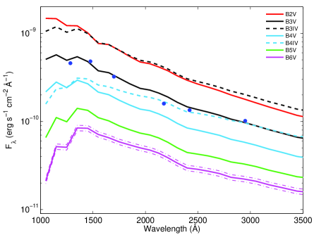
Figure 2: IUE measurements and tested model spectral types for 48 Librae. IUE measurements are represented by filled blue circles, and the synthetic SEDs for various spectral types are shown by solid or dashed lines as indicated in the legend. The dash-dot lines above and below the B6V model represent the SED computed at the distance given by $p+\sigma$ and $p-\sigma$, respectively.

Stars of spectral types later than B3 were simply not luminous enough to match the observed flux levels, even accounting for the increased luminosity as the star evolves, while a more evolved B3 star (i.e. of luminosity class IV or III) was too luminous to match the observations. In Figure 2, the UV portion of some of the tested model spectral types are compared with the IUE measurements. In all cases, the model spectra are computed assuming the central star is surrounded by a dense disk, and that the system is oriented at 85°. Main-sequence stars of spectral type B2($M_{\star}=8.62M_{\odot}$) to B6 are shown in solid lines. In the case of the B6V model, we also show the effect of changing the distance to the star within $\pm 1\sigma$ of the Hipparcos parallax. The lower dash-dotted line represents $p-\sigma$ and the upper dash-dotted line represents $p+\sigma$. Each model experiences the same spread in its flux by adjusting the distance in this manner, and thus it can be seen that errors in the distance do not imply a significant error in the stellar parameters. The best fit to the data is clearly given by the B3V model SED. A more evolved B3 star (i.e. a B3IV star) is also shown (black dashed line) on the plot, but it is obviously too luminous to reproduce the observations. The B4IV model (blue dashed line) appears to match some of the IUE data points, but it is noticeably underluminous in the far UV portion of the SED. Note also that the overall shape of the model B4IV SED is somewhat flattened and does not reflect the observed shape. Models of B5IV and B6IV stars (not shown) suffered this same discrepancy, and were systematically underluminous to reproduce the observations.

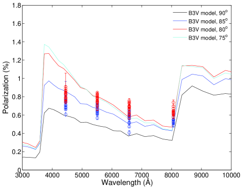
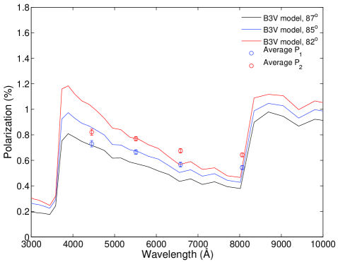
Figure 3: Polarization of 48 Librae. Left panel: continuum linear polarization measurements shown with models created at different inclination angles, as indicated in the legend. Blue dots ($P_{\rm{1}}$) represent the observations corrected by the ISP given in Štefl et al. (2012), and red dots ($P_{\rm{2}}$) represent the observations corrected by the ISP given in Draper et al. (2014). Right panel: Averaged $P_{\rm{1}}$ and $P_{\rm{2}}$ continuum linear polarization measurements with their averaged errors, bracketed by models at 82°and 87°. The best average representation is given by the model created at 85°.

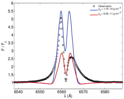
Figure 4: H$\alpha$ profile of 48 Librae. The observed profile, shown in open circles, has each of its peaks matched individually by unperturbed disk models of initial density as specified in the legend.

The observed IR fluxes are well matched by a disk whose initial density is $\rho_{0}=8.8\times 10^{-11}$ g cm^-3 at the stellar surface (Figure 1) and oriented at 85°  (Figure 3). We again note that this density represents only the average (unperturbed) initial disk density. While our first estimate of the average initial disk density was obtained by fitting the IR portion of the SED, we further constrained this value by consulting the H$\alpha$ profile shown in Figure 4. The final value of the average initial disk density was obtained in an efficient manner by modelling the individual peak heights of this profile and then averaging the two values. Notably, the density derived from the H$\alpha$ line was in good agreement with the value obtained by fitting the IR portion of the SED. The H$\alpha$ line, however, was more sensitive to small changes in density, thus helping to better constrain the model. The H$\alpha$ observations and the modelling procedure are discussed further in Section  4.3.

A B3V central star with a disk whose average density was obtained by the methods described above matches the UV (IUE data) and visible portion (Strömgren $ubvy$, Johnson $UBV$, and Tycho-2 data) of the SED exceedingly well. The Balmer jump at $\lambda=3646$Å  is well matched by a model oriented at 85°, which is further supported by the polarization measurements (see next section). The only data point not well matched in this portion of the SED is the Strömgren $u$ flux at $\lambda=3500$Å. However, we note that this measurement has a large associated error, and that the upper limit of the measurement is well matched by our model. Furthermore, the Johnson $U$ measurement, which is at a similar wavelength but has a much smaller error, is also well fit by our model, suggesting that the flux near this wavelength is indeed closer to the upper limit of the Strömgren $u$ measurement.

The infrared portion of the SED merits some discussion. In the near IR (Tycho-2 data), the assumed average disk density again fits the observations remarkably well. In the far IR (WISE, AKARI, and IRAS data) however, there is a small discrepancy between the unperturbed model and the observed data points. We note that the IRAS data points at 60 and 100 microns are only upper limits to the fluxes at those wavelengths (Waters et al., 1987) and should not be given much weight in determining the best disk density. The IRAS measurements at 12 and 25 microns, in addition to the WISE and AKARI data points, however, all show an improved fit when the perturbed model is applied to the SED.

48 Librae is one of only a few Be stars to have a radio (APEX data) measurement. The APEX measurement is of particular interest because it is well matched by both the unperturbed and perturbed models, and it falls more or less in line with the other data points in the SED. Vieira et al. (2015) discussed the effects of truncation on the IR SED. According to their Fig. 11, disk truncation alters the slope of the IR SED at wavelengths for which the radius of the pseudo-photosphere, which is the disk region vertically optically thick in the continuum, is of the order of the truncation radius. The fact that our model reproduces well the SED up to radio wavelengths suggests that 48 Librae is an isolated Be star, i.e. it does not experience disk truncation by a companion.

4.2 Polarization

As shown in Carciofi et al. (2009), the continuum linear polarization levels provide a strong constraint on the inclination angle $i$ of the star+disk system. The left panel of Figure 3 shows 14 polarization observations, all obtained within the most recent $V/R$ cycle, at $\lambda$ = 4450, 5510, 6580, and 8060Å. The observations in this plot have been corrected by two different ISP values, as discussed in Section 2.4. The considerable spread in the observed polarization level at each wavelength is to be expected, as polarization levels are extremely sensitive to the changing density configurations in the disk that occur with $V/R$ variations (Halonen & Jones, 2013) and to short-term variations in the disk feeding rate (Haubois et al., 2014). As done in our fitting of the SED, we analyze the polarization by attempting to match it with an unperturbed model. The predicted polarization level of the unperturbed model that fits the SED (Figure 1) is shown for four different inclination angles: 75°, 80°, 85°, and 90°. At $\lambda=4450$Å , the $P_{\rm{1}}$ data points cluster around the 85°  model or slightly lower, while the $P_{\rm{2}}$ data points centre on the 85°  model. We give some preference to using the $P$ values at $\lambda=4450$Å , as it can clearly be seen in the figure that the model changes most noticeably at this wavelength, whereas the differences in models become consistently smaller at longer wavelengths. As shown in the right panel of Figure 3, the average of each reduction of the polarization is fairly well fit by the model at 85°, although at $\lambda=4450$Å  the average of $P_{\rm{1}}$ is better fit by a slightly higher inclination angle (87°), and at $\lambda=5510$Å, the average of $P_{\rm{2}}$ is better fit by a slightly lower inclination angle (82°). The averages of $P_{\rm{1}}$ and $P_{\rm{2}}$ are not very well fit at $\lambda=6580$Å, but it can be seen from the left panel that adopting a lower inclination angle does not improve the fit to these two points; in fact, the model created at 75°  has a lower $P$ value at this wavelength than the model created at 80°. All data points are fairly well fit by any of the models at $\lambda=8060$Å, but we note that the models experience a fair bit of degeneracy at that point, as the differing inclination angles cause almost no discernable difference in the models. We therefore give preference to fitting the data at $\lambda=4450$ and $5510$Å. By bracketing the lowest $P_{\rm{1}}$ value at $\lambda=4450$Å  and the highest $P_{\rm{2}}$ value at $\lambda=5510$Å, we determine the inclination angle to be approximately $85\pm 3$°.

4.3 The H$\alpha$ Profile

The H$\alpha$ profile shown in Figure 4 was obtained 2005-04-01. The violet peak has $F/F_{c}\approx 5.2$ while the red peak has $F/F_{c}\approx 2.5$, yielding a $V/R$ value of $\approx 2.1$, which is very close to the maximum value of $V/R$ reported in 2006. This indicates that, at the time of the observation, 48 Lib’s disk is oriented such that the overdense region is moving toward the observer almost in its entirely, while the underdense region is receding from the observer.

To quantify the densities required to produce each peak height, we model them separately. The violet peak height is best represented by a model with an initial density $\rho_{0}=1.1\times 10^{-10}$ g cm^-3, and the red peak height is reproduced by a model with an initial density $\rho_{0}=6.5\times 10^{-11}$g  cm^-3. Averaging the two densities, we obtain $\rho_{0}=8.8\times 10^{-11}$g  cm^-3. We note that an axisymmetric model of initial density $\rho_{0}=1.1\times 10^{-10}$ g cm^-3 reproduces the large peak at some times, but would, on average, produce profiles too large to match the observation, while the initial density of $\rho_{0}=6.5\times 10^{-11}$g  cm^-3 produces profiles too weak on average. This can be seen by comparing Figure 4, where the lower density profile has peaks only at about $F/F_{c}\approx 2.7$ and the higher density profile has peaks at $F/F_{c}\approx 5.5$, with the centre panel of Figure 7 where $V=R$ and $F/F_{c}$ is about 3.6 or 3.7. However, these values of initial density can be interpreted as a good first order approximation to the upper and lower limits to the range of densities in our model that produces a reasonable facsimile of the observations.

4.4 $V/R$ Variations

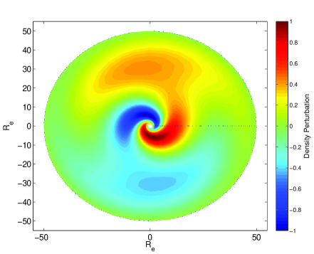
Figure 5: Density perturbation pattern as predicted by the 2D global oscillation code with $\alpha$ = 0.76. The disk is viewed from above, with a void at the centre representing the location of the central star, and the $x$- and $y$-axes give the distance from the central star in units of stellar radii. The density perturbation is normalized by the unperturbed value, with red regions corresponding to overdense regions and blue regions corresponding to underdense regions.

The model disk structure predicted by the 2D global oscillation code is shown in Figure 5. This model is obtained by superimposing an $m=1$ oscillation on the unperturbed disk of initial density $\rho_{0}=8.8\times 10^{-11}$g cm^-3. The values of the input parameters $k_{2}$, $\eta$, $\epsilon$, $\alpha$, $\dot{M}$ are listed in Table 5. The value of $k_{2}$ is taken from Papaloizou et al. (1992), but is, in theory, a free parameter. The adopted values of $\eta$ and $\epsilon$ are those that were used the successful modelling of $\zeta$ Tau in Carciofi et al. (2009). The value of $\alpha$ is a free parameter that may vary between 0 and 1, with lower $\alpha$ values usually corresponding to more confined modes. The parameter $\alpha$ ultimately governs the mass decretion rate, $\dot{M}$. We adopted the value of $\alpha=0.76$ as it was shown in Escolano et al. (2015) that higher $\alpha$ values tend to better reproduce Be star observables, and it yields a mass decretion rate that is consistent with what is expected to maintain a dense and extended disk such as the one surrounding 48 Lib. The oscillation produced by these five parameters has a period of 12.13 years, which is in good agreement with the average observed $V/R$ cycle length of $\sim$10 years.

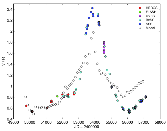
Figure 6: $V/R$ cycle of 48 Librae. Filled circles represent $V/R$ observations, with different colours representing different instruments used to collect the H$\alpha$ line spectra, as given in the legend. The model H$\alpha$ $V/R$ cycle computed from the perturbed disk shown in Figure 5 is overplotted in open circles. The model cycle has been shifted in phase to align with the observed cycle, has been plotted over the same time period as the observations.

48 Librae’s most recent $V/R$ cycle is shown in Figure 6. One full cycle is defined as the time between the $V/R$ minimums. The first such minimum occurs shortly after MJD 50000, and the second occurs shortly after MJD 560000, for a total cycle length of approximately 6000 days, or $\sim$16.5 years. The $V/R$ cycle corresponding to one full precession of the model disk is also shown in Figure 6. Given the complexity of the model, and the large number of input parameters, the agreement between the observed and model cycles is quite remarkable; the overall behaviour of the observed cycle is matched quite well in a qualitative sense. There are, however, some manifest discrepancies between the model and the observations. Firstly, the amplitude of the $V/R$ cycle is not matched by the model. Our model displays the same minimum $V/R$ ($\approx 0.5$) as the observed one, and its maximum $V/R$ ($\approx 2.1$) is close to the observed one ($\approx 2.4$), but it does not attain the same value. Furthermore, the width of the main peak is too broad in the model, in the sense that the model predicts a rise in $V/R$ slightly before it is observed, and the decline of $V/R$ also happens more slowly in the model than what is observed.

In an attempt to determine if the amplitude of the $V/R$ could be matched by a greater disk density, we computed a model with the initial disk density increased by 30%. This resulted in only a marginally larger maximum $V/R$ value ($\approx 2.15$), but produced a $V/R$ cycle with drastically different behaviour that no longer matched the general features of the observation.

A sample of model H$\alpha$ profiles are compared with observed profiles (obtained at the Lowell observatory) in Figure 7. The left panel shows an observation obtained 2007-03-26 and shows the near maximum $V>R$ configuration in the disk. This configuration is fairly well matched by our model, although the red peak is somewhat overestimated by the model. The centre panel shows an observation obtained 2009-07-10, when $V\approx R$. The peak intensity is quite well matched; however, the central absorption is not nearly strong enough in our model. Finally, the right panel shows an observation obtained 2012-06-22 when $V>R$, and as in the leftmost panel, the weaker peak is again overestimated by the model.

In each of the three panels in Figure 7, one clear discrepancy in the model is the inability to fit the observed line wings. The very broad wings that are seen in the observations are thought to arise mainly from non-coherent scattering, which is not included in our model, and thus this discrepancy is to be expected.

An additional discrepancy common to all of the panels in Figure 7 is that the central absorption of the model is too small to match the observations. This feature most likely arises from the fact that our model assumes a pure hydrogen composition for the disk. As shown in Sigut & Jones (2007), including metals in the disk model can lead to a predicted temperature distribution that differs significantly from the one that is predicted for a pure hydrogen disk. Since our model does not account for the the cooling effect that metals provide, the temperature in the outer parts of the model disk is most likely overestimated. This, in turn, leads to an overestimation of the flux in the outer portion of the model disk, and artificially fills in the central absorption.

We further compared the model and observed H$\alpha$ line profiles by considering their EWs. To do so, we employed the carefully measured EWs of the Lowell Observatory H$\alpha$ observations. As mentioned in Section 2.3, these observations were taken on 30 nights between 2005 and 2015, and samples most of the most recent $V/R$ cycle. It was found that the EW of the H$\alpha$ line varied between $\sim-26$ Å  and $\sim-18$ Å  during that time, with the average of all the measurements being -21.8 Å. Averaging the EWs of the H$\alpha$ line profiles obtained from one full model $V/R$ cycle, we obtain the value -21.3 Å. This indicates that the density obtained by modelling each of the peaks individually is approximately correct, and reproduces the strength of the H$\alpha$ emission.

5 Summary and Discussion

By examining and modelling several key observables simultaneously, we obtained a self-consistent description of 48 Librae and its dense, extended circumstellar disk. Our final stellar and disk parameters are summarized in Table 5.

One of the first goals of this work was to model the SED of 48 Librae in order to conclusively determine the star’s spectral type; accurately determining the central star’s parameters is crucial to modelling the entire system, as the photoionizing radiation provided by the central star affects all other aspects of the model. The SED, however, cannot be modelled in its entirety without considering the disk. For this reason, we opted to achieve a first estimate of the average disk density by separately modelling the two peaks of one representative H$\alpha$ profile with simple, axisymmetric models, and then averaging the two initial densities that were obtained. This proved to be an efficient method of determining the average initial density of the disk. The SED was well matched by the axisymmetric model created with this average initial density, and applying the perturbation actually improved the SED fit. From the SED fitting, we conclude that the central star is of spectral type B3V, and it is surrounded by a disk of average initial density $\rho_{0}=8.8\times 10^{-11}$ g cm^-3.

The modelling of the SED also gives an indication of the inclination of the system. For a disk of a given density distribution, the adopted inclination will affect the size of the Balmer jump at $\lambda=3646$Å  (Bjorkman & Carciofi, 2005). The SED was best fit by models oriented at 85°, and this $i$ was then confirmed by examining the polarization levels. This finding supports the hypothesis that shell stars are Be stars viewed in a nearly edge-on configuration.

The values of the densities obtained in this work are of some interest, as they are all considered to be quite high. This suggests 48 Lib’s disk is unusually dense, which is congruent with its very large flux in H$\alpha$ and its strong IR excess. The density contrast in the two regions responsible for the violet and red H$\alpha$ emission peaks is also remarkable. Our analysis implies that the overdense region is more than 1.7 times as dense as the underdense region.

An additional interesting result of this work is the observed radio flux of 48 Librae, which implies a large disk size. Using the pseudo-photosphere model of Vieira et al. (2015) we estimate that at 870$\mu$m the size of the disk pseudo-photosphere of our best fit model is about 35$R_{\star}$, which implies that the disk cannot be smaller than this value. In any case, this finding is not inconsistent with 48 Librae being an isolated Be star.

The 2D global oscillation code predicts a perturbed disk with a period of $\sim$12 years, which is in good agreement with previously observed $V/R$ cycle lengths observed for 48 Librae, although the most recent $V/R$ cycle appears to have had a period of $\sim$16 years. Furthermore, the general behaviour of the $V/R$ cycle is well matched by the model, and the EWs of the H$\alpha$ lines produced by the model are also in excellent agreement with the observed ones. Some aspects of the model $V/R$ variations do require some improvement, however. Firstly, the amplitude of the $V/R$ cycle could not be matched by our model, and testing a model with increased initial density did not rectify this. In fact, the model with increased initial density displayed entirely different behaviour in its model $V/R$ cycle, which indicates that small changes in the model can have large and unanticipated effects. Secondly, the main peak of the $V/R$ cycle is too broad in our model. Interestingly, this effect was also observed by Carciofi et al. (2009) when they applied the 2D oscillation model to $\zeta$ Tau. It seems this phenomenon may be a feature of the 2D model, as Escolano et al. (2015) were able to properly reproduce the peak of the $V/R$ cycle by employing a 2.5D oscillation. It is our intention to test this hypothesis in a future work.

One further aspect of the observations that was not particularly well matched by the model is the shapes of the H$\alpha$ line profiles shown in Figure 7. As mentioned above, we plan to employ a 2.5D (or, ideally, a fully 3D) oscillation in a future work, which should increase the realism of our models and perhaps resolve this issue as well. A factor that may prove more important in improving the appearance of the H$\alpha$ profiles, however, is the use of a version of HDUST that employs a realistic solar chemical composition. This version of HDUST is currently being developed. Finally, we also hope to improve and refine all aspects of our model by employing H$\alpha$ and near-IR interferometry to place tighter constraints on the disk geometry and density configuration in a future work. This first attempt at applying a global oscillation scenario to 48 Lib has proven quite successful at reproducing most of the observables, and executing the improvements suggested above should lead to a much better understanding of the stellar and circumstellar components of this unusual Be star.

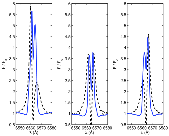
Figure 7: Comparison of observed (dashed line) and model (solid blue line) H$\alpha$ profiles at three different phases. Left panel: the observed H$\alpha$ profile, obtained on March 26, 2007, is in a $V>R$ configuration, and the model is at $\varphi=252\arcdeg$. Centre panel: the observed H$\alpha$ profile, obtained on July 10, 2009, is in a $V$ = $R$ configuration, and the model is at $\varphi=66\arcdeg$. Right panel: the observed H$\alpha$ profile, obtained on June 22, 2012, is in a $V<R$ configuration, and the model is at $\varphi=36\arcdeg$.

Table 1: Photometric Observations

Instrument	$\lambda$	Flux	Error
and/or Filter	(Å)	(erg s-1 cm-2 Å-1)	(erg s-1 cm-2 Å-1)
IUE 1250-1300	1285	4.583E-10	2.529E-11
IUE 1450-1500	1475	4.800E-10	2.451E-11
IUE 1675-1725	1700	3.226E-10	1.275E-11
IUE 2150-2200	2175	1.593E-10	1.389E-11
IUE 2395-2445	2420	1.343E-10	1.111E-11
IUE 2900-3000	2950	1.015E-10	4.856E-12
Strömgren u	3448	1.747E-11	4.033E-11
Johnson U	3571	5.475E-11	2.171E-12
Strömgren v	4110	7.771E-11	3.860E-11
TYCHO B	4280	7.695E-11	9.922E-13
Johnson B	4378	7.678E-11	1.773E-12
Strömgren b	4663	6.473E-11	7.003E-12
TYCHO V	5340	4.260E-11	3.531E-13
Johnson V	5466	4.021E-11	8.519E-13
Strömgren y	5472	3.976E-11	4.321E-12
2MASS J	12350	2.858E-12	5.687E-13
2MASS H	16620	1.326E-12	9.772E-14
2MASS Ks	21590	6.242E-13	1.149E-14
WISE W1	33526	1.484E-13	1.038E-14
WISE W2	46028	8.947E-14	4.532E-15
IRAS 12$\mu$m	101465	4.688E-15	1.875E-16
WISE W3	115608	3.176E-15	3.510E-17
AKARI IRC L18W	176095	1.053E-15	1.430E-17
IRAS 25$\mu$m	217265	3.772E-16	4.149E-17
WISE W4	220883	5.349E-16	1.083E-17
IRAS 60$\mu$m	519887	4.436E-17	$\cdots$
IRAS 100$\mu$m	952971	6.800E-17	$\cdots$
APEX	8700000	7.306E-21	1.796E-21

Table 2: H$\alpha$ Spectroscopic Observations

Telescope	Instrument	Date	JD	No. of	Resolving
Name	Name		2400000+	Spectra	Power
ESO 50 cm, Ondřejov 2 m	heros	1995–2003	49 788–52 725	18	20 000
Wendelstein 80 cm	flash	2000-05-25	51 690	1	20 000
ESO/VLT-Kueyen	uves	2001-07-11	52 101	2	60 000
ESO/VLT-Kueyen	uves	2008-04-03	54 559	9	60 000
John S. Hall 1.1 m	sss	2005–2015	53 462–57 114	49	10 000
BeSS Database
CN212, FS128	lhires1	2001–2004	52 048–53 126	11	6 000
C8, C11, C12	lhires3	2005–2014	53 430–56 802	19	17 000
CNC212	Echelle V1	2008-05-01	54 588	1	8 000
SC12	lhires-a12t	2008	54 645, 54 743	2	6 000
C11	eShel	2009–2010	54 907–55 301	3	10 000
CNC212, C11, C14	lhires3	2010–2015	55 388–57 131	16	15 000
C9	lhires3	2012-05-12	56 060	1	12 000
C14	lhires3	2012-06-20	56 098	1	11 000

Table 3: Polarimetric Observations

Obs.	MJD	Filter	$\lambda$ (Å)	$P_{\rm{1}}$ (%)	$P_{\rm{2}}$ (%)
1	54975.649	B	4450	0.777 $\pm$ 0.019	0.868 $\pm$ 0.019
	54975.660	V	5510	0.733 $\pm$ 0.020	0.830 $\pm$ 0.020
	54975.682	R	6580	0.603 $\pm$ 0.021	0.699 $\pm$ 0.021
2	55012.623	B	4450	0.762 $\pm$ 0.013	0.866 $\pm$ 0.008
	55012.578	V	5510	0.714 $\pm$ 0.013	0.847 $\pm$ 0.006
	55012.601	R	6580	0.646 $\pm$ 0.009	0.742 $\pm$ 0.009
3	55334.752	B	4450	0.827 $\pm$ 0.029	0.888 $\pm$ 0.029
	55334.761	V	5510	0.699 $\pm$ 0.025	0.796 $\pm$ 0.023
	55334.772	R	6580	0.559 $\pm$ 0.032	0.615 $\pm$ 0.016
	55334.764	I	8060	0.579 $\pm$ 0.035	0.738 $\pm$ 0.028
4	55396.521	B	4450	0.754 $\pm$ 0.017	0.849 $\pm$ 0.017
	55396.515	V	5510	0.700 $\pm$ 0.018	0.810 $\pm$ 0.021
	55396.503	R	6580	0.519 $\pm$ 0.017	0.632 $\pm$ 0.011
	55396.492	I	8060	0.546 $\pm$ 0.014	0.644 $\pm$ 0.007
5	55427.399	B	4450	0.710 $\pm$ 0.017	0.833 $\pm$ 0.017
	55427.415	V	5510	0.632 $\pm$ 0.023	0.744 $\pm$ 0.023
	55427.428	R	6580	0.408 $\pm$ 0.025	0.692 $\pm$ 0.025
	55427.437	I	8060	0.524 $\pm$ 0.020	0.617 $\pm$ 0.020
6	55441.388	B	4450	0.756 $\pm$ 0.018	0.791 $\pm$ 0.009
	55441.396	V	5510	0.696 $\pm$ 0.022	0.787 $\pm$ 0.022
	55441.403	R	6580	0.594 $\pm$ 0.020	0.693 $\pm$ 0.018
	55441.409	I	8060	0.522 $\pm$ 0.022	0.616 $\pm$ 0.024
7	55695.701	B	4450	0.608 $\pm$ 0.022	0.739 $\pm$ 0.017
	55695.686	V	5510	0.619 $\pm$ 0.013	0.741 $\pm$ 0.004
	55695.696	R	6580	0.563 $\pm$ 0.005	0.666 $\pm$ 0.006
8	56408.085	B	4450	0.819 $\pm$ 0.150	0.909 $\pm$ 0.150
	56408.102	V	5510	0.641 $\pm$ 0.038	0.738 $\pm$ 0.038
	56408.118	R	6580	0.589 $\pm$ 0.041	0.685 $\pm$ 0.041
	56408.137	I	8060	0.530 $\pm$ 0.017	0.624 $\pm$ 0.017
9	56408.245	B	4450	0.661 $\pm$ 0.007	0.750 $\pm$ 0.007
	56408.252	V	5510	0.568 $\pm$ 0.018	0.664 $\pm$ 0.018
	56408.262	R	6580	0.474 $\pm$ 0.016	0.570 $\pm$ 0.016
	56408.270	I	8060	0.488 $\pm$ 0.020	0.580 $\pm$ 0.020
10	56505.053	B	4450	0.736 $\pm$ 0.009	0.826 $\pm$ 0.009
	56505.060	V	5510	0.654 $\pm$ 0.005	0.751 $\pm$ 0.005
	56505.070	R	6580	0.599 $\pm$ 0.008	0.695 $\pm$ 0.008
	56505.080	I	8060	0.554 $\pm$ 0.004	0.646 $\pm$ 0.004
11	56517.025	B	4450	0.676 $\pm$ 0.011	0.766 $\pm$ 0.011
	56517.038	V	5510	0.608 $\pm$ 0.009	0.704 $\pm$ 0.009
	56517.048	R	6580	0.511 $\pm$ 0.011	0.607 $\pm$ 0.011
	56517.057	I	8060	0.507 $\pm$ 0.010	0.601 $\pm$ 0.010
12	56839.992	B	4450	0.746 $\pm$ 0.017	0.836 $\pm$ 0.017
	56839.996	V	5510	0.722 $\pm$ 0.025	0.817 $\pm$ 0.025
	56840.001	R	6580	0.661 $\pm$ 0.024	0.758 $\pm$ 0.024
	56840.008	I	8060	0.578 $\pm$ 0.012	0.671 $\pm$ 0.012
13	56888.979	B	4450	0.705 $\pm$ 0.006	0.796 $\pm$ 0.006
	56888.984	V	5510	0.645 $\pm$ 0.008	0.759 $\pm$ 0.008
	56888.990	R	6580	0.581 $\pm$ 0.021	0.668 $\pm$ 0.021
	56888.998	I	8060	0.549 $\pm$ 0.009	0.633 $\pm$ 0.009
14	57142.114	B	4450	0.688 $\pm$ 0.016	0.777 $\pm$ 0.016
	57142.103	V	5510	0.683 $\pm$ 0.012	0.779 $\pm$ 0.012
	57142.108	R	6580	0.631 $\pm$ 0.016	0.727 $\pm$ 0.016
	57142.120	I	8060	0.603 $\pm$ 0.012	0.696 $\pm$ 0.012

Table 4: Adopted Stellar and Disk Parameters of 48 Librae

Parameter	Value	Ref.
Stellar Parameters
Spectral Type	B3V	1,2
$M_{\star}$	6.07 $M_{\odot}$	1,3
$R_{\rm{p}}$	3.12 $R_{\odot}$	4
$R_{\star}$	4.12 $R_{\odot}$	1
$L_{\star}$	1100 $L_{\odot}$	4
$W$	0.74	1
$\beta_{GD}$	0.17	5
Disk Parameters
$\rho_{0,V}$	1.1 $\times 10^{-10}$ g cm-3	1
$\rho_{0,R}$	6.5 $\times 10^{-11}$ g cm-3	1
$\rho_{0,avg}$	8.8 $\times 10^{-11}$ g cm-3	1
$V/R$ Parameters
$P$	12.13 yr	1
$k_{2}$	0.006	6
$\eta$	5.74 $\times 10^{-2}$	7
$\epsilon$	0.1	7
$\alpha$	0.76	1
$\dot{M}$	8.27 $\times 10^{-10}M_{\odot}$ yr-1	1
Geometrical Parameters
$i$	$85\pm 3$°	1
$d$	$143\begin{subarray}{c}+5\\ -10\end{subarray}$ pc	8

References. — (1) this work; (2) Underhill (1953); (3) Harmanec (1988); (4) Georgy et al. (2013); (5) Espinosa Lara & Rieutord (2012); (6) Papaloizou et al. (1992); (7) Carciofi et al. (2009); (8) van Leeuwen (2007).

References

- Abt et al. (2002) Abt, H. A., Levato, H., & Grosso, M. 2002, ApJ, 573, 359
- Ballereau et al. (1995) Ballereau, D., Chauville, J., & Zorec, J. 1995, A&AS, 111, 423
- Bayo et al. (2008) Bayo, A., Rodrigo, C., Barrado Y Navascués, D., et al. 2008, A&A, 492, 277
- Bjorkman & Carciofi (2005) Bjorkman, J. E., & Carciofi, A. C. 2005, in Astronomical Society of the Pacific Conference Series, Vol. 337, The Nature and Evolution of Disks Around Hot Stars, ed. R. Ignace & K. G. Gayley, 75
- Brown & Verschueren (1997) Brown, A. G. A., & Verschueren, W. 1997, A&A, 319, 811
- Carciofi & Bjorkman (2006) Carciofi, A. C., & Bjorkman, J. E. 2006, ApJ, 639, 1081
- Carciofi & Bjorkman (2008) —. 2008, ApJ, 684, 1374
- Carciofi et al. (2008) Carciofi, A. C., Domiciano de Souza, A., Magalhães, A. M., Bjorkman, J. E., & Vakili, F. 2008, ApJ, 676, L41
- Carciofi et al. (2009) Carciofi, A. C., Okazaki, A. T., Le Bouquin, J.-B., et al. 2009, A&A, 504, 915
- Chauville et al. (2001) Chauville, J., Zorec, J., Ballereau, D., et al. 2001, A&A, 378, 861
- Chen & Marlborough (1994) Chen, H., & Marlborough, J. M. 1994, ApJ, 427, 1005
- Cox (2000) Cox, A. N. 2000, Allen’s Astrophysical Quantities, 4th edn. (London: The Athlone Press)
- Cranmer (2005) Cranmer, S. R. 2005, ApJ, 634, 585
- Delaa et al. (2011) Delaa, O., Stee, P., Meilland, A., et al. 2011, A&A, 529, A87
- Draper et al. (2014) Draper, Z. H., Wisniewski, J. P., Bjorkman, K. S., et al. 2014, ApJ, 786, 120
- Escolano et al. (2015) Escolano, C., Carciofi, A. C., Okazaki, A. T., et al. 2015, A&A, 576, A112
- Espinosa Lara & Rieutord (2012) Espinosa Lara, F., & Rieutord, M. 2012, A&A, 547, A32
- Faraggiana (1969) Faraggiana, R. 1969, A&A, 2, 162
- Georgy et al. (2013) Georgy, C., Ekström, S., Granada, A., et al. 2013, A&A, 553, A24
- Güsten et al. (2006) Güsten, R., Nyman, L. Å., Schilke, P., et al. 2006, A&A, 454, L13
- Hall et al. (1994) Hall, J. C., Fulton, E. E., Huenemoerder, D. P., Welty, A. D., & Neff, J. E. 1994, PASP, 106, 315
- Halonen & Jones (2013) Halonen, R. J., & Jones, C. E. 2013, ApJS, 208, 3
- Harmanec (1988) Harmanec, P. 1988, Bulletin of the Astronomical Institutes of Czechoslovakia, 39, 329
- Haubois et al. (2014) Haubois, X., Mota, B. C., Carciofi, A. C., et al. 2014, ApJ, 785, 12
- Hauck & Mermilliod (1998) Hauck, B., & Mermilliod, M. 1998, A&AS, 129, 431
- Helou & Walker (1988) Helou, G., & Walker, D. W., eds. 1988, Infrared astronomical satellite (IRAS) catalogs and atlases. Volume 7: The small scale structure catalog, Vol. 7
- Høg et al. (2000) Høg, E., Fabricius, C., Makarov, V. V., et al. 2000, A&A, 355, L27
- Houk & Smith-Moore (1988) Houk, N., & Smith-Moore, M. 1988, Michigan Catalogue of Two-dimensional Spectral Types for the HD Stars. Volume 4, Declinations to
- Ishihara et al. (2010) Ishihara, D., Onaka, T., Kataza, H., et al. 2010, A&A, 514, A1
- Jaschek & Jaschek (1992) Jaschek, C., & Jaschek, M. 1992, A&AS, 95, 535
- Jaschek et al. (1980) Jaschek, M., Jaschek, C., Hubert-Delplace, A.-M., & Hubert, H. 1980, A&AS, 42, 103
- Jones et al. (2011) Jones, C. E., Tycner, C., & Smith, A. D. 2011, AJ, 141, 150
- Klement et al. (2015) Klement, R., Carciofi, A. C., Rivinius, T., et al. 2015, ArXiv e-prints, arXiv:1510.01229
- Kraus et al. (2012) Kraus, S., Monnier, J. D., Che, X., et al. 2012, ApJ, 744, 19
- Lee et al. (1991) Lee, U., Osaki, Y., & Saio, H. 1991, MNRAS, 250, 432
- Lesh (1968) Lesh, J. R. 1968, ApJS, 17, 371
- Magalhães et al. (1984) Magalhães, A. M., Benedetti, E., & Roland, E. H. 1984, PASP, 96, 383
- Magalhães et al. (1996) Magalhães, A. M., Rodrigues, C. V., Margoniner, V. E., Pereyra, A., & Heathcote, S. 1996, in Astronomical Society of the Pacific Conference Series, Vol. 97, Polarimetry of the Interstellar Medium, ed. W. G. Roberge & D. C. B. Whittet, 118
- Meilland et al. (2007) Meilland, A., Stee, P., Vannier, M., et al. 2007, A&A, 464, 59
- Mennickent & Vogt (1988) Mennickent, R. E., & Vogt, N. 1988, A&AS, 74, 497
- Mermilliod & Mermilliod (1994) Mermilliod, J.-C., & Mermilliod, M. 1994, Catalogue of Mean UBV Data on Stars
- Molnar (1972) Molnar, M. R. 1972, ApJ, 175, 453
- Murakami et al. (2007) Murakami, H., Baba, H., Barthel, P., et al. 2007, PASJ, 59, 369
- Neiner et al. (2011) Neiner, C., de Batz, B., Cochard, F., et al. 2011, AJ, 142, 149
- Okazaki (1997) Okazaki, A. T. 1997, A&A, 318, 548
- Okazaki & Negueruela (2001) Okazaki, A. T., & Negueruela, I. 2001, X-ray Astronomy: Stellar Endpoints, AGN, and the Diffuse X-ray Background, 599, 810
- Panoglou et al. (submitted) Panoglou, D., Carciofi, A. C., Vieira, R. G., et al. submitted, MNRAS
- Papaloizou et al. (1992) Papaloizou, J. C., Savonije, G. J., & Henrichs, H. F. 1992, A&A, 265, L45
- Porter & Rivinius (2003) Porter, J. M., & Rivinius, T. 2003, PASP, 115, 1153
- Rivinius et al. (2013) Rivinius, T., Carciofi, A. C., & Martayan, C. 2013, A&A Rev., 21, 69
- Sana et al. (2012) Sana, H., de Mink, S. E., de Koter, A., et al. 2012, Science, 337, 444
- Shakura & Sunyaev (1973) Shakura, N. I., & Sunyaev, R. A. 1973, A&A, 24, 337
- Sigut & Jones (2007) Sigut, T. A. A., & Jones, C. E. 2007, ApJ, 668, 481
- Skrutskie et al. (2006) Skrutskie, M. F., Cutri, R. M., Stiening, R., et al. 2006, AJ, 131, 1163
- Slettebak (1982) Slettebak, A. 1982, ApJS, 50, 55
- Slettebak et al. (1975) Slettebak, A., Collins, II, G. W., Parkinson, T. D., Boyce, P. B., & White, N. M. 1975, ApJS, 29, 137
- Touhami et al. (2013) Touhami, Y., Gies, D. R., Schaefer, G. H., et al. 2013, ApJ, 768, 128
- Underhill (1953) Underhill, A. B. 1953, Publications of the Dominion Astrophysical Observatory Victoria, 9, 363
- Underhill (1966) Underhill, A. B., ed. 1966, Astrophysics and Space Science Library, Vol. 6, The early type stars
- Štefl et al. (2012) Štefl, S., Le Bouquin, J.-B., Carciofi, A. C., et al. 2012, A&A, 540, A76
- van Leeuwen (2007) van Leeuwen, F. 2007, A&A, 474, 653
- Vieira et al. (2015) Vieira, R. G., Carciofi, A. C., & Bjorkman, J. E. 2015, MNRAS, 454, 2107
- von Zeipel (1924) von Zeipel, H. 1924, MNRAS, 84, 665
- Waters et al. (1987) Waters, L. B. F. M., Cote, J., & Lamers, H. J. G. L. M. 1987, A&A, 185, 206
- Wheelwright et al. (2012) Wheelwright, H. E., Bjorkman, J. E., Oudmaijer, R. D., et al. 2012, MNRAS, 423, L11
- Wright et al. (2010) Wright, E. L., Eisenhardt, P. R. M., Mainzer, A. K., et al. 2010, AJ, 140, 1868