Split scores: a tool to quantify phylogenetic signal in genome-scale data

Abstract

Detecting variation in the evolutionary process along chromosomes is increasingly important as whole-genome data become more widely available. For example, factors such as incomplete lineage sorting, horizontal gene transfer, and chromosomal inversion are expected to result in changes in the underlying gene trees along a chromosome, while changes in selective pressure and mutational rates for different genomic regions may lead to shifts in the underlying mutational process. We propose the split score as a general method for quantifying support for a particular phylogenetic relationship within a genomic data set. Because the split score is based on algebraic properties of a matrix of site pattern frequencies, it can be rapidly computed, even for data sets that are large in the number of taxa and/or in the length of the alignment, providing an advantage over other methods (e.g., maximum likelihood) that are often used to assess such support. Using simulation we explore the properties of the split score, including its dependence on sequence length, branch length, size of a split and its ability to detect true splits in the underlying tree. Using a sliding window analysis, we show that split scores can be used to detect changes in the underlying evolutionary process for genome-scale data from primates, mosquitoes, and viruses in a computationally efficient manner. Computation of the split score has been implemented in the software package SplitSup. [phylogenetic trees, split scores, genome-scale data analysis, general Markov model, matrix flattenings, singular value decomposition]

Building on recent mathematical progress in understanding phylogenetic models from an algebraic perspective, we develop here a new tool for empirical analysis, the split score. This score allows one to compare support in a sequence alignment for different possible splits (i.e., bipartitions of taxa, corresponding to putative edges in trees). Through a “sliding window” analysis, we demonstrate how this can be used to investigate a variety of biologically interesting changes in evolutionary processes along the genome, such as differing evolutionary trees, inversions, and changes in selective constraints.

Although similar analyses have been performed using full maximum likelihood inference of trees (Hobolth et al., 2007; Boussau et al., 2009), the split score offers several advantages over previous methods: (1) it focuses directly and solely on a split, and not on the split as inferred with a full tree and model parameters, (2) it is theoretically justified for models of sequence evolution beyond those routinely assumed, in particular requiring neither a stationary distribution, nor homogeneity of the substitution process over the tree, and (3) its computation is extremely fast, even for a large number of taxa, making it a viable tool for exploratory analyses. While some caution is necessary in interpreting and comparing split scores, our empirical examples show they can provide biological insight.

The thread of ideas we build on to develop the split score is perhaps not widely known to empiricists, though the field of phylogenetics has benefitted in numerous ways from the application of ideas from algebra and geometry. One of the earliest algebraically-based methods for inferring an evolutionary tree was “evolutionary parsimony,” put forth by Lake (1987), in which simple weighted sums of estimated site pattern probabilities were used to infer phylogenetic relationships. Viewing these sums as linear (i.e., first degree) polynomials, they are an instance of phylogenetic invariants — polynomials whose values should be zero when evaluated at the site pattern probabilities for a particular tree and substitution model. Independently, Cavender and Felsenstein (1987) proposed higher degree polynomial invariants as a tool for inference, but their detailed work was with a 2-state model, and not developed for practical application.

Following these initial works, the ideas were extended in various ways (Cavender, 1989; Fu and Li, 1992; Evans and Speed, 1993; Steel et al., 1993; Fu, 1995; Hendy and Penny, 1996; Allman and Rhodes, 2003). However, the use of invariants in empirical phylogenetic studies was rare. Simulations showed Lake’s linear invariants needed significantly longer data sequences to produce accurate estimates than traditional methods such as maximum likelihood (Hillis et al., 1994; Huelsenbeck, 1995), while understanding of higher degree invariants was still insufficient for their practical use. Despite this unpromising start, it is interesting to note that similar invariant methods are currently the basis of widely-used analysis tools, though this connection is rarely mentioned in the current literature. For example, the ABBA-BABA test (Durand et al., 2011), used to detect introgression and hybrid speciation in empirical data, is based on the difference in the empirical frequencies of two types of site patterns among four taxa (ABBA-like patterns and BABA-like patterns).

Indeed, the use of an algebraic framework for phylogenetic inference and theory advancement gained traction only after mathematical understanding of higher-degree polynomial relationships in site pattern probabilities was further developed. Using ideas primarily from algebraic geometry, large classes of informative phylogenetic invariants for a variety of models were identified and characterized. Often these non-linear invariants can be linked to local features in a tree, such as a vertex or edge Sturmfels and Sullivant (2005); Allman and Rhodes (2008); Rhodes and Sullivant (2012).

Such advances led to the development of arrangements of the probability distribution of site patterns on large trees into arrays of reduced dimensions, by “flattening” the distribution according to edges or nodes within a phylogenetic tree. For example, an edge flattening is a matrix whose rows correspond to possible site patterns for the taxa on one side of the edge, and columns to possible site patterns on the other. An entry of the matrix is the probability of observing the amalgamated site pattern for its row and column. Flattenings were first presented broadly to the research community in the 2004 arXiv preprint of Allman and Rhodes (2008), to understand the ideal of all invariants for the general Markov (GM) model on trees.

Importantly, the study of algebraic characteristics of such flattenings led to the development both of methods for establishing identifiability of gene tree topologies and associated parameters, and to the development of algorithms for inferring the tree. For example, rank conditions on matrix flattenings were used by Allman and Rhodes (2006) to identify tree topologies for $k$-class mixtures ($k=1,2,3$) of GM models and independently by Eriksson (2005) for the non-mixture GM model. The latter work also made the first use of the singular value decomposition (SVD) of matrix edge flattenings, as a tool for measuring approximate matrix rank, to develop an invariant-based algorithm for tree construction. Although performance of that early algorithm was disappointing, several recent works have explored the use of the SVD of flattenings for tree inference in ways that appear much more promising (Casanellas and Fernandez-Sanchez, 2007, 2015).

These algebraically-motivated ideas have also been applied to the multi-locus setting, in which estimation of a species trees under the coalescent model is the goal. Again using the ideas of flattenings and rank approximations, Chifman and Kubatko (2015) derived invariants for the $4$-taxon species trees under the coalescent model based on the site pattern probability distribution, leading to both establishment of identifiability of the species tree, and an inference method called SVDQuartets (Chifman and Kubatko, 2014) that is implemented in PAUP* (Swofford, 2016). Other work in this area includes invariant-based methods of establishing identifiability of the species tree from collections of gene tree topologies Allman et al. (2011a) or from clade probabilities Allman et al. (2011b).

Rather than consider inference of an entire phylogeny, here we turn our attention to the use of tools arising from an algebraic phylogenetic framework to learn about various features of large-scale genomic data. In particular, we consider the case of data arising from a single gene phylogeny and show how a statistic based on the singular value decomposition can be used to measure support for particular phylogenetic relationships in that data. We study the behavior of this statistic using simulated data to demonstrate the impact of factors such as the length of the gene, the branch lengths in the true underlying gene tree, and the substitution model.

We then demonstrate how our statistic can be applied to whole-genome data to extract features of the underlying evolutionary model, both with regard to the tree structure and with regard to the substitution process, by applying our method to three empirical data sets. The first is the data of Patterson et al. (2006), which consists of whole-genome data for five primate species. These data demonstrate the ability of our method to detect the gene-level variability predicted by the coalescent process. The second example uses whole-genome data for a species complex of Anopheles gambiae mosquitoes from Fontaine et al. (2015), for which our method is able to detect the region of a known chromosomal inversion. Finally, we apply our method to genome-scale data from 29 whole-genomes of Cassava Brown Streak Virus and Ugandan Cassava Brown Streak Virus, demonstrating that the method captures variation in the substitution process from gene-to-gene across the viral genome. These examples highlight that a major advantage of our method is the rapid computation time, with an entire chromosome being analyzed in a matter of minutes.

We begin by providing the mathematical theory underlying our proposed method. Readers interested primarily in the application of the methodology can skip to the Methods section of the paper, where we present our statistic and describe how it can be used to analyze large-scale empirical data.

Theoretical Background

Basic Theory

The general Markov (GM) model of evolution of DNA sequences on trees underlies the theoretical development of our statistic, the split score. This model assumes an arbitrary probability distribution, $\boldsymbol{\pi}=(\pi_{A},\pi_{G},\pi_{C},\pi_{T}),$ describing bases at the root of the tree. In addition, to each edge, $e$, of the tree (directed away from the root) is associated a $4\times 4$ matrix, $M_{e}$, of conditional probabilities of the various base substitutions. No special relationships between the matrices associated to different edges is assumed; in particular, the GM model does not assume time-reversibility of the substitution process, a stationary base distribution, homogeneity of the substitution processes across the edges of the tree, nor even the existence of an underlying homogeneous continuous-time process on any edge. This model thus encompasses, but is more general than, the general time-reversible (GTR) model and its submodels which are commonly used in current data analysis. However, it lacks the across-site rate variation features that are also often combined with the GTR model in the form of invariant sites and $\Gamma$-distributed scaling factors (e.g., GTR+I+$\Gamma$).

The GM model implies that certain conditional independence statements hold for the joint distribution of bases at the leaves of the tree. These express the fact that the base substitutions that occur in a clade on a rooted tree are not affected by those occurring outside the clade, except through the sequences at the clade’s most recent common ancestor. To be more precise, pick any edge $e$ of the unrooted tree and let $v$ be one of its end nodes. Deleting $e$ from the tree breaks it into two parts, and induces a partition of the taxa $X$ into disjoint sets $X_{1}$ and $X_{2}$, the split $X_{1}|X_{2}$ associated to $e$. Then the joint distribution of bases at the leaves of the tree can be organized as a $4^{|X_{1}|}\times 4^{|X_{2}|}$ matrix $F_{e}$, with rows indexed by patterns of bases for $X_{1}$, and columns by patterns of bases for $X_{2}$. This is the edge flattening of the joint distribution along $e$. The conditional independence statement above is then formulated mathematically as the fact that $F_{e}$ has a factorization

$$F_{e}=M_{1}^{T}DM_{2}$$

where $D$ is a $4\times 4$ diagonal matrix with entries giving the base distribution at $v$, and the $M_{i}$ are $4\times 4^{|X_{i}|}$ stochastic matrices giving probabilities of the bases at the taxa in $X_{i}$ conditioned on the bases at $v$. As a consequence of the matrix factorization, the rank of the matrix $F_{e}$ will be at most 4.

One can as well consider any split $X_{1}|X_{2}$ of the taxa, whether associated to an edge or not, and then construct a split flattening $F$ of the joint distribution according to it. If the split does not arise from an edge of the tree, then $F$ does not have the simple structure above. Under very mild and plausible assumptions on the nature of the model parameters, this implies the rank of the matrix $F$ is larger than 4 Allman and Rhodes (2006); Eriksson (2005).

The central idea of our method is to view an empirical distribution of bases in data sequences as an approximation of the true distribution, and then use a measure of how close a split flattening of this empirical distribution is to a matrix of rank 4 as an indication of whether the split is supported or not. If we have exact distributions arising from the general Markov model, our measure will be zero for splits displayed on the tree, and positive for splits not displayed.

Rank-4 matrix approximations, the SVD, and split scores

One way of measuring the size of a matrix uses the Frobenius norm; if $M=(m_{ij})$, then

$$||M||=||M||_{F}=\left(\sum_{i,j}m_{ij}^{2}\right)^{1/2}.$$

The associated distance between two matrices $F$ and $G$ is then $||F-G||$. Adopting these measures means there is a good tool to determine the closest rank-4 matrix to a given matrix, using the singular value decomposition (SVD) and software developed for computing it.

The SVD of an $m\times n$ real matrix $F$ is a factorization

$$F=U\Sigma V^{T},$$

where $U$ and $V$ are $m\times m$ and $n\times n$ orthogonal matrices, and $\Sigma$ is a $m\times n$ diagonal matrix with entries

$$\sigma_{1}\geq\sigma_{2}\geq\cdots\geq\sigma_{\min(m,n)}\geq 0,$$

the singular values of $F$. By the Eckart-Young Theorem Eckart and Young (1936), under the Frobenius norm the closest rank-4 approximation to a matrix $F$ is $\tilde{F}=U\tilde{\Sigma}V^{T}$ where $\tilde{\Sigma}$ is obtained from $\Sigma$ by zeroing out all but the 4 largest singular values. Moreover the Frobenius distance between $F$ and $\tilde{F}$ is

$$||F-\tilde{F}||=\left(\sum_{i=5}^{\min(m,n)}\sigma_{i}^{2}\right)^{1/2}.$$

As a measure of split support, then, we define the split score

$$S(X_{1}|X_{2})=S(F)=\left(\frac{\sum_{i=5}^{\min(m,n)}\sigma_{i}^{2}}{\sum_{i=1}^{\min(m,n)}\sigma_{i}^{2}}\right)^{1/2}\ =\\ \ \left(1-\frac{\sum_{i=1}^{4}\sigma_{i}^{2}}{\sum_{i=1}^{\min(m,n)}\sigma_{i}^{2}}\right)^{1/2},$$

where $F$ is the $(X_{1}|X_{2})$-flattening of the empirical distribution. The denominator is introduced so that the result is independent of the scaling of $F$. Thus the formula may be applied either to $F$, or to the unnormalized matrix of counts leading to it. The split score takes values in the interval from 0 to 1. A score of 0 indicates $F$ is a rank 4 matrix, and a positive score indicates that it is not. Implicit in this theory is that split scores are defined for “gapless” alignments. We exclude any site at which one or more of the taxa has a gap, or missing data of any kind.

To compute split scores, one must compute singular values of potentially large matrices. Since the Frobenius norm is related to the singular values by

$$||F||=\left(\sum_{i=1}^{\min(m,n)}\sigma_{i}^{2}\right)^{1/2},$$

the formula above can also be written as

$$S(X_{1}|X_{2})=S(F)=\left(1-\frac{\sum_{i=1}^{4}\sigma_{i}^{2}}{||F||^{2}}\right)^{1/2}.$$

Using this formula, only the 4 largest singular values are needed. This observation provides significant computational advantage, as there are good algorithms for computing a specified number of the largest singular values with significantly faster runtimes than if all are needed.

If the number of taxa is large, and sequence lengths are as typical in alignable sequences, any split flattening $F$ will be a large and sparse matrix, i.e., most entries will be zero. Computation of singular values of such matrices requires a sparse encoding of them in software, and special packages for the SVD computation. Fortunately, these are highly developed as the SVD has many applications in scientific computing.

Although one might suppose that computations would be slowed considerably by increasing the number of taxa, thus exponentially increasing the size of the flattening matrix, this is not the case. Since site patterns appearing in finite-length sequence data tend to be those more strongly reflecting the underlying tree, the sparsity of the matrix tends to be patterned, with many zero rows or columns which can be ignored. Even though increasing sequence length does lead to more non-zero entries in the matrix, this happens slowly due to the very low probability of many site patterns. Finally, the iterative routines used for computing singular values converge most quickly to determine the few largest values, which are precisely the ones we need. Any detailed analysis of theoretical running time is complicated by how the matrix sparsity and the size of the singular values depend upon the phylogenetic model parameters, number of taxa, and sequence length; still, one should expect fast performance.

In practice, we have found that assembling the sparse flattening matrix dominated the computation time, since each sparse encoding requires a scan of all unique site patterns in the alignment. Nonetheless, all the necessary computations to produce split scores for reasonable size data sets can be performed quickly enough that runtime is of little concern. For instance, for simulated data on a 100-taxon tree (not shown) with sequence length 1000 bp (respectively 10,000 bp) computing all 97 scores for splits displayed on the tree took 0.186 seconds (respectively 8.68 seconds) on a MacBook Pro 3.1 GHz with 16 GB of memory. Computation time was similar for scores of 97 random splits of the same sizes. See also the applications section for an example of timing on empirical data.

Interpretation of split scores

When applied to an empirical joint distribution, a low split score (close to 0) indicates support for that split, and a higher score (close to 1) indicates lack of support. However, a variety of factors, such as split size, edge lengths, sequence length, and model fit affect the interpretation of $S(X_{1}|X_{2})$. Some of these effects will be illustrated through the simulations described below. Here we focus attention on one theoretical principle concerning the size of the split and its influence on the score.

Some of the effect of the size of a split (the number of taxa included in each of the two groups) on the split score has a clear mathematical explanation. The space of $m\times n$ matrices has dimension $mn$, while the subset of those that have rank 4 or less forms an object of dimension $4(m+n)-16$. (The simplest way to see this is to count free parameters in the LU matrix factorization of an $m\times n$ matrix of rank 4.)

Applied to $F$, for $|X|=N$, $|X_{i}|=N_{i}$, we have $m=4^{N_{1}}$, $n=4^{N_{2}}$, so

$$mn=4^{N},\ \ 4(m+n)-16=4(4^{N_{1}}+4^{N-N_{1}})-16.$$

This last expression is easily seen to decrease as $N_{1}$ goes from 1 to $\lfloor\frac{N}{2}\rfloor$, where it has a minimum. That is, the dimension of the set of matrices of rank at most 4 drops with the size of $N_{1}$ until $N_{1}=N_{2}$ if $N$ is even, or $N_{1}=N_{2}-1$ if $N$ is odd. The smaller the dimension of the set of rank 4 matrices is, the greater the distance should be between this set and a random perturbation of one of its elements. (To see this, imagine moving a point in $3$-space that lies on a line $\ell$ contained in a plane $\mathcal{P}$ a fixed distance in a random direction. The movement typically leaves the point further from the line $\ell$ than from $\mathcal{P}$, since more of the motion will be in a direction within the plane than in the direction of the line.) Thus even for splits arising from the tree on which data was simulated, we should expect larger split scores for splits that are closer to balanced. Indeed, this geometric understanding explains why the tree reconstruction algorithm of Eriksson (2005) performs poorly in practice, tending to create trees with a preponderance of cherries and small clades. By comparing splits of different sizes, splits with size $N_{1}=2$ or more generally $N_{1}=k$ where $k$ is small are preferred and bias the reconstruction.

We note that this dimensional understanding can be developed into a theoretical correction to the split score which, at least asymptotically, can overcome the dependence on split size. However, we found this correction inadequate to substantially improve comparability of the scores, so do not present it here.

Methods

As described above, our method involves computation of a split score associated with a putative edge $e$ of a phylogenetic tree. If $X$ denotes the set of taxon names, then a split $X_{1}\mid X_{2}$ of the taxa is a bipartition of $X$ into two disjoint sets $X_{1}$, $X_{2}$. When $k=|X_{1}|\leq|X_{2}|$ we call such a split a $k$-split.

For a $N$-taxon unrooted binary tree $T$, there are $2N-3$ true splits on $T$, corresponding to edges of $T$. Of these, $N$ are trivial splits (the $1$-splits which appear on all $T$), which we no longer consider. If $T$ is the true tree describing the evolutionary history of the taxa under study, then all other splits are false splits, since they do not correspond to edges in $T$.

Suppose now that $e$ is a putative edge in the true tree relating data sequences and that $e$ corresponds to the split $X_{1}\mid X_{2}$. We can arrange the observed counts of site patterns from the alignment of a single gene into a $4^{|X_{1}|}\times 4^{|X_{2}|}$ matrix, called a flattening and denoted by $F_{e}$ as above, where the rows of $F_{e}$ are indexed by possible nucleotides for each of the taxa in $X_{1}$ and the columns are indexed by possible nucleotides for each of the taxa in $X_{2}$. We assess support for the specified edge as a true edge in the underlying phylogenetic tree by measuring how close the matrix $F_{e}$ is to the nearest rank 4 matrix, based on the theory described above. We measure closeness using the split score

$$S(X_{1}|X_{2})=\left(1-\frac{\sum_{i=1}^{4}\hat{\sigma}_{i}^{2}}{||F||^{2}}\right)^{1/2}$$ (1)

where $\hat{\sigma_{i}}$ refers to the $i^{th}$ singular value obtained from $F_{e}$ and $||F||$ is as defined above.

We have implemented the computation of split scores in the program SplitSup written jointly by the authors in the C programming language using the publicly available SVDLIBC library. This code, available at https://github.com/eallman/SplitSup/, reads an alignment in PHYLIP format and returns either (i) a set of scores corresponding to a list of user-provided splits; or (ii) the values of a split score in a sliding-window across the length of the alignment. For option (ii), the user specifies the window size, the number of nucleotides to move the window for the next computation, and the minimum number of sites without gaps required to compute scores in each window. The SVD computations have been sped up significantly by using a binary encoding of site patterns, and a sparse encoding of the flattening matrices.

We next describe our methods for assessing the utility of the split score using both simulated and empirical data. Although all simulations described below were carried out using the Jukes-Cantor model, we note that similar results can be obtained under any of the commonly used substitution models that are submodels of the GTR model, or more generally any submodel of the GM model. Indeed, this generality is one of the key features of the split score.

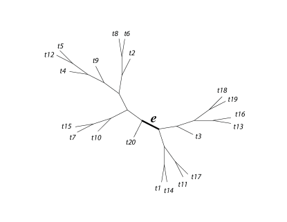
Figure 1: 20-taxon tree used for simulations.

Simulation Study 1

Our first simulations were designed to test that our split score can detect true splits in the underlying tree, under ideal circumstances. We also investigated how the magnitude and spread of splits scores varies, and if there are qualitative differences between true and false splits. To accomplish this, we used SeqGen (Rambaut and Grassly, 1997) to generate a single data set under the Jukes-Cantor model for the tree in Figure 1 with all branch lengths set to $0.05$. For each value $k=2,3,\dots,10$, we computed the split score for each of the $\binom{20}{k}$ possible splits and then generated histograms for the scores for $k$-splits. The $N-3$ non-trivial true $k$-splits were marked on the appropriate histograms.

This enabled us to compare the score values for true and false splits, understand the distribution of split scores, and gain insight into the effect of split size on the score; that is, how does proximity of an edge to the tips of the tree or nearer the middle of the tree affect the score’s value? To refine our understanding further, we classified false splits by how “far” they were from a true split. For example, if the true split of size $9$ in a tree consisted of $X_{1}=$ {taxa 1-9} and $X_{2}=$ {taxa 10-20}, then we say that a split with $X_{1}=$ {taxa 1-8, taxon 10} and $X_{2}=$ {taxon 9, taxa 11-20} is one swap away from a true split.

Simulation Study 2

Our next simulations were performed to explore the effects of sequence length and branch length on the distribution of scores. On the $20$-taxon tree shown in Figure 1 we used SeqGen to simulate 100 data sets of varying sequence lengths (500 bp; 5,000 bp; and 50,000 bp) with all branch lengths set to $0.05$ under the Jukes-Cantor model. To test the effect of tree diameter, we simulated 100 replicate data sets of 500 bp under the Jukes-Cantor model with all branch lengths set to $0.0125$, $0.025$, $0.05$. We then compared empirical distributions of split scores for all true splits.

To improve our understanding of the effect of metric depth on the distribution of a particular split score, 100 replicate data sets of length 500 bp were next simulated under the Jukes-Cantor model with various scalings. Attention was focused on the $9$-split induced by edge $e$ pictured in Figure 1. Scores for this true split were computed on data simulated when all the branch lengths were scaled by a fixed factor, every branch was scaled except $e$, only edge $e$ was scaled, and when all edges to one side of the split were scaled by the factor. In short, with either a subset or all of the branches rescaled, split scores were compared.]

A last simulation was a hybrid of the previous two. Here we focused attention on a true $9$-split and a true $2$-split in the tree, and carefully selected other bipartitions of the 20 taxa that we considered ‘close’ ($1$-swap or $2$-swap) or ‘distant’ (random). This made for a total of seven splits (four $9$-splits, three $2$ splits), {t9, s9-1, s9-2, s9-R, t2, s2-1, s2-R}, which we now describe.

The true $9$-split, t9, is the one pictured in Figure 1. By interchanging taxa $3$ and $20$ we obtain split s9-1 (for nine split, one swap away from t9). By interchanging taxa {1, 3} and taxa {10, 20}, we obtain split s9-2 (for nine split, a two swap away from t9). Because the swaps here interchange only a few “topologically close” taxa, these false splits are expected to be difficult to distinguish from true splits. The split s9-R (for Random nine split) has taxa {2 3 6 7 14 15 16 18 19} on one side of the bipartition, and should be easier to distinguish from a true one.

The split t2 is the true $2$-split grouping together taxa {1 14}. The split s2-1 groups together taxa {1 11}, resulting from a 1-swap of “topologically close” taxa, and is expected to be hard to distinguish as false. The split s2-R groups taxa {1 8} together, and since these are far from one another in the tree, should be easier to distinguish as false.

For the simulations, 100 replicate data sets were made under the Jukes-Cantor model on the tree (Fig 1) with branch lengths set to 0.05, and sequence lengths of 500 bp, 5000 bp, and 50000 bp. Additionally, fixing the sequence length at 500 bp, 100 replicate data sets were simulated when the branch lengths were set to 0.0125, 0.025, and 0.05. For each parameter setting and each replicate, splits scores were computed for the seven splits.

To test that the true split scores were the lowest, or closest to the lowest, we computed the difference between the scores of the false splits and the true split (e.g., compute score(s9-1) - score(t9)). A positive difference indicates that the true score is the smallest and the magnitude of the difference reveals how close in value are the scores of nearby and distant splits under a variety of model settings.

Simulation Study 3

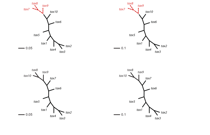
Figure 2: 10-taxon trees used for sliding window simulations in Simulation Study 3. (See online for color.)

We evaluated our method on genome-scale data using a sliding-window computation of split scores for contiguous sections along the alignment. To test this approach, we used Seq-gen and the Jukes-Cantor model to simulate data for an alignment of total length 20,000 bp, by concatenating four chunks of 5,000 bp simulated on the $10$-taxon model trees shown in Figure 2. The first two trees are topologically identical, but the branch lengths of $0.05$ in tree 1 are doubled to a value of $0.1$ in tree $2$. The second two trees are also topologically identical with all branch lengths $0.05$ and $0.1$ respectively; however, these trees are topologically distinct from trees 1 and 2 in that taxa $7$ and $10$ in tree 1 have been interchanged to obtain the topology of trees 3 and 4. In particular taxa $\{7,8,9\}$ form a true $3$-split in trees 1 and 2, and taxa $\{8,9,10\}$ form a true $3$-split in trees 3 and 4. The sliding window analysis computed and compared scores for the $3$-splits $\{7,8,9\}$ and $\{8,9,10\}$ using a window of size $500$ bp at at intervals of 100 bp (slide offset size). This means the start sites for each 500 bp window were $1,101,201,$ etc.

Application to Empirical Data

Our simulations demonstrate that the split score can be used to detect both changes in topological relationships and changes in the underlying evolutionary process. We now demonstrate the utility of the split score in practice by application to three empirical data sets. Note first that alignments of empirical data often have sites in which some sequences have gaps, which are excluded for the computation of the split score. If gapped sites are too numerous this can result in little data being left to analyze, and split scores can be misleading. It is therefore wise to require a minimum number of non-gapped sites to eliminate spurious signals. We specify the minimum number of sites required in each of analyses below.

Primate Data– We applied the sliding window method to the data set of Patterson et al. (2006), which consists of whole-genome data for human, chimp, gorilla, orangutan, and macaque. (Data at http://genetics.med.harvard.edu/reich/Reich_Lab/ Datasets_-_Patterson_2006.html) We considered the data for chromosome 7 ($\sim$ 1.9-million bp), and applied our method with a window size of $10,000$ bp, a slide size of $1,000$ bp, and required that at least $500$ (= 5%) non-gap sites were present in a window for a score to be computed. We computed scores for the three possible splits of the taxa human, chimp, gorilla, and orangutan. For each window examined, we determined which of the three splits gave the lowest split score, and we plotted the results using different colors/shading to indicate which split each region of the genome supported most strongly. The primary process leading to variation in the genealogy across a chromosome for these taxa is expected to be the process of incomplete lineage sorting. Thus, we expect that the majority of the data will support the human-chimp $|$ gorilla-orangutan split most strongly, with approximately equal support for the other two splits.

Mosquito Data – Fontaine et al. (2015) carried out a phylogenomic analysis of whole genomes from the Anopheles gambiae species complex. (Data at http://dx.doi.org/10.5061/dryad.tn47c.) We considered the analysis of chromosome 2L, and utilized an approximately 37.5-million bp alignment of a subset of this chromosome for four species: An. gambiae, An. coluzzii, An. arabiensis, and An. christyi (the outgroup). As with the primate data, we considered all three possible splits, and carried out the sliding window analysis with a window size of $10,000$ bp, a slide size of $1,000$ bp, and required that at least 500 (= 5%) non-gap sites were present in a window for a score to be computed. Fontaine et al. (2015) found that gene flow between the ancestor of the An. gambiae-An. coluzzii clade occurred with An. arabiensis, revealing an interesting pattern in the region of a known chromosomal inversion on chromosome 2L. In particular, because both An. coluzzii and An. arabiensis experienced the inversion, while An. gambiae did not, the tree supporting a sister relationship between An. coluzzii and An. arabiensis is expected to dominate in this region, while An. gambiae and An. coluzzii are expected to be sister taxa elsewhere along the chromosome. We thus assess whether our analysis can detect the region of this chromosomal inversion.

CBSV Data – Alicai et al. (2016) recently collected complete viral genomes for 14 samples of Cassava Brown Streak Virus (CBSV) and 15 samples of Ugandan Cassava Brown Streak Virus (UCBSV). The viral genomes consist of 10 distinct genes, and we considered sequence data for the entire genome (i.e., all 10 genes) for all 29 individual samples. (See Figure 3 of Alicai et al. (2016) for Genbank accession numbers.) The published phylogenetic analysis based on these data indicate that CBSV has an accelerated rate of evolution compared to UCBSV, which matches field observations indicating increased virulence for these strains. We applied our method with a window size of $500$ bp, a slide size of $100$ bp, and required that at least 100 non-gap sites were present in a window for a score to be computed. We considered the single split that partitioned the sequences into CBSV versus UCBSV, and evaluated changes in the score across the genome as an indicator of which genes may be involved in the shift in evolutionary rate of CBSV. This example highlights application of our method to a data set of more than four taxa when gene boundaries are known.

Results

Simulation 1 Results

Identifying true splits: Displayed in Figure 3 are split scores distributions of all $k$-splits for $k=2,4,6,9$. (Histograms for other values of $k$ are not shown but fit the pattern seen here). The values of our scores for true splits in the tree are shown with red dots. For all $k=2,3,\dots,10$, scores for true splits from the generating tree are the smallest in the distributions. This shows that even for simulated data of modest size (500 bp) the split score picks out true splits in the tree.

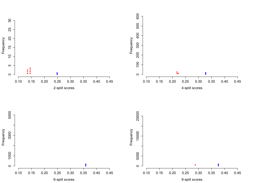
Figure 3: The distributions of $k$-split scores for $k=2,4,6,9$ are shown. Scores were computed for all $\binom{20}{k}$ possible splits for a data set of 500 bp generated under the Jukes-Cantor model on the tree in Figure 1 with all branch lengths set to $0.05$. These distributions are left-tailed, and the mean increases and the standard deviation decreases as $k$ increases. Behavior for other values of $k$ is similar. The red dots show the scores for the true $k$-splits in the tree, which are the smallest in the data. (There are no $6$-splits in the tree.) The blue line segment marks the mean. The $x$-axis is the same on all subplots, but the $y$-axis scales differ vastly because $\binom{20}{k}$ increases as $k$ varies from $2$ to $10$. (See online for color.)

Split scores distributions: The histograms (Fig. 3) also shed light on the distribution of split scores. Notably, as $k$ increases, the mean, which is shown in blue in Figure 3, of the scores increases and the spread of the scores narrows.

As observed above, there are solid theoretical reasons why the size $k$ of a $k$-split should affect the range of score values for both true and false splits, with smaller $k$ giving rise to smaller scores. This phenomenon can be explained in part by our algebraic-geometric understanding of the dimension of the space of $m\times n$ matrices of rank $4$ or less that fundamentally underlies the development of our methods.

Effect of split size: In Table 1, the mean and standard deviations are displayed for all $\displaystyle\binom{20}{k}$ $k$-splits for a single data set, emphasizing in numerical terms the effect of $k$ on the distributions. While one might naively expect scores for all size splits to be comparable, there is a clear pattern of larger scores when the split is closer to being “balanced” with equal numbers of taxa on each side of the edge. This prompts a caution to any practitioner: scores for different split sizes should not be compared.

Mean and standard deviation of $k$-split scores

Split size	mean	std
2	0.2487	0.0398
3	0.2997	0.0261
4	0.3276	0.0202
5	0.3459	0.0167
6	0.3585	0.0146
7	0.3672	0.0131
8	0.3730	0.0122
9	0.3762	0.0117
10	0.3773	0.0115

Table 1:

Effect of “closeness” to a true split The histogram in Figure 4 displays scores for all possible 10-splits for data simulated from the tree in Figure 1. The coloring illuminates how scores are distributed for false splits that differ from the true $10$-split $X_{1}|X_{2}$ on the tree in Figure 1 by swapping $\ell$ taxa between the sets, for various $\ell$. Observations are colored according to how many taxa need to be swapped from a false split to produce the single true 10-split. Note that splits that require only one or two swaps tend to have lower scores, while those requiring three or four swaps tend to have higher scores. Splits requiring more than four swaps to obtain the true split generally have higher scores. Thus, the magnitude of a score gives an indication of how near that split is to being a true split in the underlying tree.

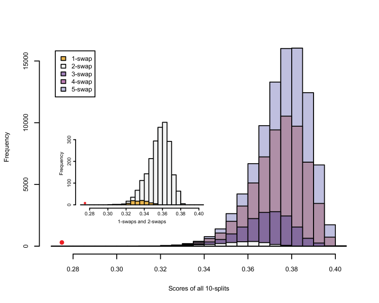
Figure 4: Distribution of scores of all 10-splits from data simulated on the tree of Figure 1 under the Jukes-Cantor model with edge lengths 0.05. The score for the one true split of size 10 lies to the left of all others and is shown as a red dot. For false splits, colors indicate the number of individual taxa that are swapped between the sets of the true split. (See online for color.)

Simulation 2 Results

Effect of sequence length: Figure 5a shows split scores for two edges of the metric tree displayed in Figure 1, where each branch has length $0.05$. Since the values of scores depends on the size of a split (cf. theoretical discussion and Simulation 1 results), boxplots are displayed for two true splits of $T$. The first split is a $9$-split and corresponds to edge $e$ in Figure 1. The second true split is a $2$-split. The scores are computed from simulations of sequences of increasing length, and show that scores of true splits decrease as the sequence length grows. This behavior is expected, assuming good model fit, since as the sequence length grows, the empirical distribution more closely matches the theoretical one, and the score for a true split should approach the theoretical value 0. Shorter sequences produce empirical distributions that are typically poorer approximations to the asymptotics of the model.

Figure 6a shows boxplots for the difference of false and true split scores (i.e., false-split-score minus true-split-score) for 100 replicate data sets. Across all sequence lengths (500 bp, 5000 bp, 50000 bp), we see that the difference is positive, indicating the true split score is always the smallest, even when the false split differs little from the true split. (This held for sequences as short as 150 bp; results not shown.) Moreover, for all lengths the magnitude of the score difference increases as the false splits deviate more from the true one. These simulations illustrate the ability of the split score to detect the deviation of a false split from a true split at a broad range of sequence lengths.

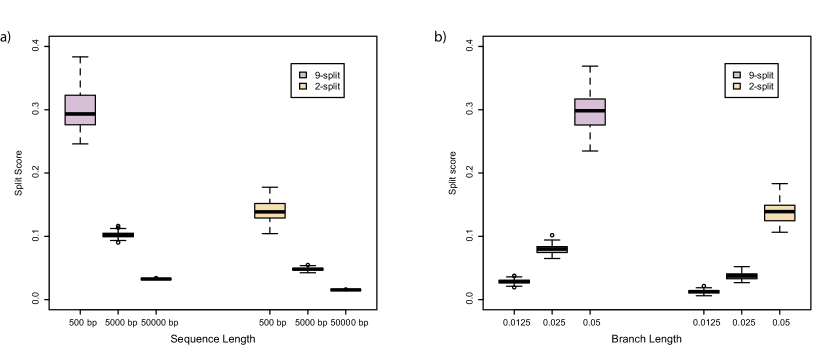
Figure 5: (a) Split scores associated to two edges on tree $T$ (Fig. 1) from sequences of length 500, 5000, 50000 bp simulated on $T$ according to the Jukes-Cantor model, with all edge lengths 0.05. Each boxplot represents scores for 100 data sets. This illustrates that split scores for true splits decrease with sequence length. (b) The distribution of split scores for two true splits in three trees are shown. The three trees are topologically identical (Fig. 1) with all branch lengths set to $0.0125$, $0.025$, $0.05$ respectively. As tree diameter increases, so do the score values. This should be expected since the amount of mutation present in data scales with tree diameter, and mutation obscures the rank $4$ signal. (See online for color.)

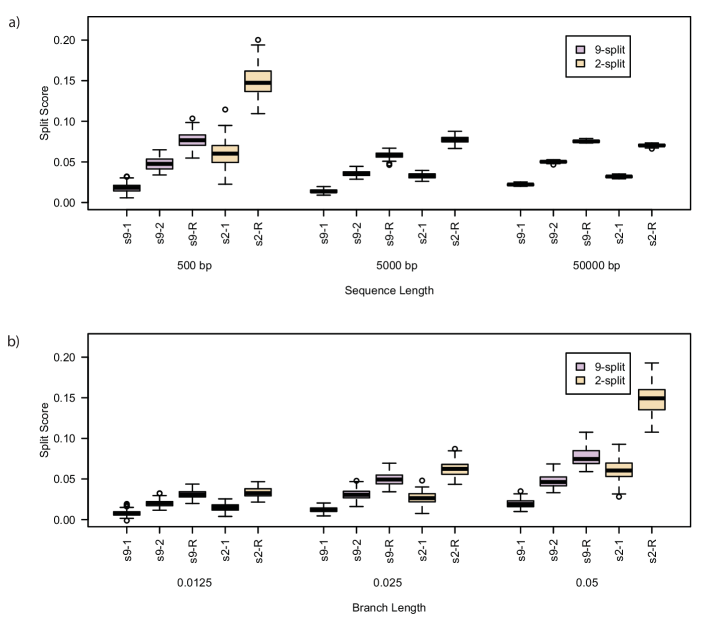
Figure 6: (a) Differences (false-split-score minus true-split-score) for true 9- and 2-splits associated to two edges of tree $T$ of Fig. 1, from sequences of length 500, 5000, 50000 bp simulated on $T$ according to the Jukes-Cantor model, with all edge lengths 0.05. Each boxplot represents differences for 100 replicates. See Simulation Study 2 methods for choices of false and true splits. In these simulations the differences were always positive, illustrating that split scores for true splits are the smallest over a range of sequence lengths. (b) Boxplots illustrating the distribution of the score differences as in (a), but with sequence length 500 bp and all branch lengths set to $0.0125$, $0.025$, $0.05$. Across this range of branch lengths, with a single exception (one simulation for s9-1 and length 0.0125), the true split score was always the smallest. (See online for color.)

Effect of tree diameter: Figure 5b shows the distribution of split scores for two true splits in three trees with identical topologies. All the trees have the topology shown in Figure 1, but branch lengths have been scaled by a fixed factor, increasing the tree diameter. As might be anticipated, the scores increase with tree diameter since longer branch lengths produce more site substitutions, diluting the signal that a flattening matrix is close to rank $4$. (With extremely long branch lengths, as saturation is reached, all scores will drop as the matrix rank goes to $1$.)

Each cluster of boxplots in Figure 6b shows score differences (false-split-score minus true-split-score) for five false splits, with branch lengths varied across simulations (0.0125, 0.025, 0.05). With a single exception (for the false 9-split closest to true, s9-1, and shortest branch lengths) the difference was positive, indicating that the score of the true split was the smallest. This indicates that the split score can distinguish true splits from false splits over a range of branch lengths.

Effect of metric depth in tree: Figure 7 shows split scores for a single edge $e$ of three trees, all with the topology shown in Figure 1, but with different branch lengths. The metric structure of the trees differs by rescaling either all or a subset of the edges (Fig. 7a, b, d), or by scaling only edge $e$ (Fig. 7c). In Figures 7a, b, d as the scaling factor is increased, the metric depth of the split in the tree (i.e, the average distance of the split from the leaves) increases. These simulations show that the split score for a true split increases with metric depth. This behavior is not surprising, and is consistent with the tree diameter scaling results of Figure 5b as the deeper an edge lies in a tree, the more obscured evidence for it may be by base substitutions nearer the leaves of the tree. In Figure 7c, only the edge $e$ is scaled, while the other branches all have length $0.025$. Since the metric depth of $e$ is held fixed, only small variation in the value of the score for the split induced by edge $e$ is observed.

Figure 7: Split scores associated to a single edge $e$ in the tree from Figure 1 computed from 500 bp sequences simulated according to the Jukes-Cantor model. The base tree in Figure 1 has all branch lengths equal to $0.025$. The single edge $e$ is the one that induces the split that bipartitions the taxa into groups of size $9$ and $11$, $\{t_{1},t_{14},t_{11},t_{17},t_{3},t_{13},t_{16},t_{19},t_{18}\}\mid\{t_{2},t_{20},t_{6},t_{8},t_{9},t_{5},t_{12},t_{4},t_{15},t_{7},t_{10}\}$. In each panel, scores for edge $e$ in the three trees are shown; these trees are topologically identical but certain branch lengths have been modified in each tree: a) All branch lengths in the trees are equal, though of differing magnitude, changing the tree diameter; b) all branch lengths EXCEPT that corresponding to edge $e$ are scaled; c) ONLY the branch length that corresponds to edge $e$ is scaled; and d) all branch lengths in the clade corresponding to taxa $\{t_{1},t_{14},t_{11},t_{17},t_{3},t_{13},t_{16},t_{19},t_{18}\}$ are scaled. In each subfigure, boxplots show distributions of scores for 100 simulated data sets.

Simulation 3 Results

Detecting changes in the evolutionary process:

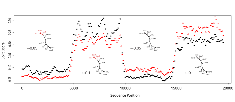
Figure 8: The values of the scores for the split {7-9} $\mid X\smallsetminus$ {7-9} are shown as red triangles, and for the split {8-10} $\mid X\smallsetminus$ {8-10} as black dots. The scores were computed by scanning along the 20,000 bp simulated genome and computing scores for the {7-9} grouping and {8-10} grouping for segments of length 500 bp at a slide size of 100 bp. For each 100 bp — $1,101,201,\dots$ — on the $x$-axis, both scores for the 500 bp window beginning at that site in the genome are plotted. The score detects both the true split in the tree used to generate the sequence data, and the shift in branch lengths. (See online for color.)

The plot displayed in Figure 8 shows that our score detects multiple changes in the evolutionary process along the genome. In particular, we see for the first 10,000 bp or so that the true split {7-9} in the tree used to generate this portion of the genome has a lower score than the false split (i.e., the red triangle is lower than the black dot). After 10,000 bp, the black dot has the smaller value; here the score captures that the sequence data for 10,000 - 20,000 bp was generated on trees with the {8-10} split.

Interestingly, our score detects not only changes in tree topology but also changes in numerical parameters of the evolutionary model. The genome sections corresponding to the first and third quarters of the sequence data (1-5,000 bp; 10,001-15,000 bp) were generated with branch lengths set to $0.05$, while the second and fourth quarters of the data (5,001-10,000 bp; 15,001-20,000 bp) were generated on trees with branch lengths $0.1$. The scores for both splits are ‘small’ for the trees with small tree diameter, and ‘large’ for the trees with large branch lengths, consistent with the results in Figure 5b.

Because our simulation and computations of scores used a sliding window of length 500 bp, but the sequence data was generated with an abrupt change in evolutionary model at sites 5,001, 10,001, and 15,001, we see a gentle rise (or fall) in the values of the scores around these transition points in our plot. This reflects that a window of size 500 bp will contain a number (400, 300, 200, 100) of sites generated from one tree, and a number (100, 200, 300, 400) of sites generated from a tree that differs in either topology or branch lengths, when the sliding window overlaps a transition site. This highlights that the selection of a window size and slide size are important parameters for analyses of this sort. Significantly, with properly chosen parameters, Figure 8 supports the hypothesis that our score can detect rough boundaries that signify shifts in the underlying evolutionary process.

Applications to Empirical Data

Primate Data – Figure 9 shows the results of the analysis of chromosome 7 for the four primate taxa. At each location along chromosome 7, a red vertical line indicates that the lowest score for that window corresponds to the split that contains the human-chimp clade, a green vertical line indicates that the lowest score corresponds to the split that contains the chimp-gorilla clade, and a blue vertical line indicates that the lowest score corresponds to the split that contains the human-gorilla clade. In this example, we expect to see variation along the chromosome as predicted by the coalescent model. In particular, because the human-chimp clade is well-established as the true phylogenetic relationship, we expect the majority of the locations along the chromosome to show this relationship with the two other relationships arising with the same, lower frequency, as is easily observed from the figure.

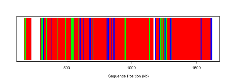
Figure 9: Application of our sliding window method to the primate data set. At each location along the chromosome, a red vertical line is drawn if the tree with the lowest score has the human-chimp clade, a green vertical line is drawn if the tree with the lowest score has the chimp-gorilla clade, and a blue vertical line is drawn if the tree with the lowest score has the human-gorilla clade. White indicates locations with excessive gaps. This data set exemplifies the expectation under the coalescent model, in that the gene tree that agrees with the species tree is expected to be more frequently observed in a set of three taxa, with the two alternative topologies occurring with equal frequency. (See online for color.)

Mosquito Data – Figure 10 shows the results of analyzing chromosome 2L for the four mosquito species. The plot is organized as described for the primate data, with the red vertical lines corresponding to the split that contains the An. gambiae-An. coluzzii clade, the blue vertical lines corresponding to the split that contains the An. gambiae-An. arabiensis clade, and the green vertical lines corresponding to the split that contains the An. coluzzii-An. arabiensis clade. The most striking feature of the graph is the center region, in which the dominant phylogeny is that containing the An. coluzzii-An. arabiensis clade. This finding agrees with the results of Fontaine et al. (2015) (see their Figure 2 and Figure 5), for which the majority of chromosome 2L shows An. gambiae and An. coluzzii to be sister taxa (indicated by the red vertical lines in Figure 10), but a chromosomal inversion in a portion of chromosome 2L in An. arabiensis leads to a closer relationship with the sample from An. coluzzii (indicated by the green vertical lines in Figure 10), which shares this inversion, over that portion of the chromosome.

This sliding window analysis was performed on a data set of size over 37.5 million bp, and sparse matrix flattenings were constructed for 37,556 windows, each of length 10,000 bp and of which 37,547 had more than 500 gapless sites so that scores were computed. The computation time for a single pairing, say the An. gambiae-An. coluzzii clade, was 7.28 minutes on a MacBook Pro 3.1 GHz processor with 16 GB of memory.

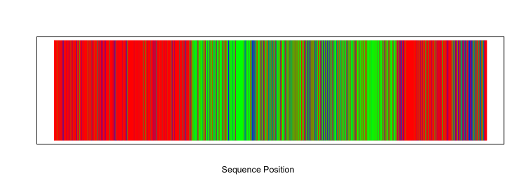
Figure 10: Application of our sliding window method to the mosquito data set. At each location along the chromosome, a red vertical line is drawn if the tree with the lowest score has the An. gambiae-An. coluzzii clade, a blue vertical line is drawn if the tree with the lowest score has the An. gambiae-An. arabiensis clade, and a green vertical line is drawn if the tree with the lowest score has the An. coluzzii-An. arabiensis clade. Some species are known to have experienced a chromosomal inversion in a portion of this region of chromosome 2L, and the method easily picks out the location of the inversion as a shift in the phylogeny. (See online for color.)

CBSV Data – Figure 11 shows the results of analyzing the 29 viral genomes, with black vertical lines delimiting boundaries between genes. Points on the plot are the score for the split that partitions the CBSV sequences from the UCBSV sequences. It is easy to see that shifts in the scores correspond largely to boundaries between genes, indicating potential shifts in the corresponding evolutionary processes governing mutation rates in CBSV vs. UCBSV, in agreement with the results of Alicai et al. (2016). This supports the results of the simulations shown in Figure 8, in which the score was shown to vary based on shifts in either the topology or the evolutionary model parameters.

Also shown on the plot are the likelihood ratio statistics for each gene for the test of differing synonymous/nonsynonymous substitution rates for the CBSV vs. UCBSV clades Yang (1997). Statistics that are significant at 5% level are indicated with a ‘*’. The split score is correlated with significance of the likelihood ratio test, in the sense that lower scores are associated with significant results for many genes. This result thus indicates variation in the evolutionary process along the genome, and hints that changes in mutation rates may be driving this variation.

Figure 11: Application our sliding window method to the CBSV data set. We evaluate support for the split that partitions the sequences into CBSV vs. UCBSV at locations across the complete viral genome. Gene boundaries are given by black vertical lines, with gene labels presented at the top of the graph. The value of the likelihood ratio statistic for testing for a difference in the ratio of synonymous vs. nonsynonymous substitutions is also given, with a ‘*’ indicating those genes for which the likelihood ratio test is significant at the 5% level.

Discussion

We have presented the split score as a means of quantifying the strength of the biological signal for specific splits on a phylogenetic tree. We demonstrate that while the score is affected by the amount of data (i.e., number of sites), the lengths of the branches in the tree, and the size of the split under consideration, the score can accurately indicate which splits are most strongly supported by a given data set. Importantly, the split score can be computed extremely rapidly, because it requires only counting of site patterns in order to construct the flattening matrix and computation of singular values from the flattening matrix. Thus, the split score is well-equipped to handle the genome-scale data sets that are being generated today. We view the split score as a valuable tool for exploratory analysis of genome-scale data sets of arbitrary size.

We have presented three empirical examples that demonstrate a practical application of our method. These involve evaluating the split score at various locations along a contiguous alignment in a “sliding window” analysis. The three examples demonstrate the varying types of biological phenomena that can be detected by an analysis such as this. The primate data show the pattern expected in a typical species tree analysis, where only incomplete lineage sorting causes variation across a chromosome. The mosquito data show that variation in the underlying evolutionary process (in this case, a chromosomal inversion) can also be detected by the method, though it is clear that the method indicates only variation in the process and does not indicate the cause of such variation. Finally, the CBSV data set demonstrates application of the method to more than four taxa (in this case, 29 taxa) and shows that the method can detect shifts in the underlying evolutionary process even when the topology remains fixed.

An important characteristic of all three empirical data sets is that they represent genome-scale data: the primate data set consists of an alignment of $\sim$1.9 million bp for 4 taxa, the mosquito data set consists of $\sim$37.5 million bp for four taxa, and the CBSV data set consists of approximately 9,000 bp for 29 taxa. In all cases, the entire sliding window analysis can be carried out within minutes on a standard desktop machine, providing a huge computational advantage over other phylogenetic tools that seek to extract similar information. We provide freely available software that requires only a PHYLIP-formatted input file and a list of splits to be evaluated to allow others to use this exploratory tool.

Detecting true splits in a tree

While it would be highly desirable to understand the dependency of the distribution of true split scores from data under a fixed model of base substitution, even with an assumption of a specific tree topology and edge lengths, this question is a complex one that is probably not addressable theoretically. (One could, of course, perform a parametric bootstrap for an approximation.) When the tree is unknown, theoretical analysis seems even more difficult. While work has been done on the distributions of singular values for certain types of random matrices, the true split flattening matrices arising from distributions along a tree, with their multinomial entries, are not covered by these results.

One approach for interpreting a split score $S(X_{1}|X_{2})$ for a split that is not known to be true or false is to compare it to the distribution of scores $S(X_{1}^{\prime}|X_{2}^{\prime}),$ $|X_{i}^{\prime}|=|X_{i}|$ for all splits of the same size computed from the same data. The false splits among these should produce larger scores than the true ones (of which there may be several.) This is borne out by Figure 3 which shows several distributions of split scores from a simulated data set on the tree in Figure 1. When true splits of a given size exist, they are markedly below the rest of the distribution. When no true splits exist, there are no such outliers. In preliminary trials, we found after some naive normalizations, such as computing z-scores, that true split scores are markedly smaller than the closest false split scores. Though we were not able to provide any probabilistic bounds on the difference between normalized true and false split scores, such ideas hold promise and need further statistical development. One step in this direction is provided by Gaither and Kubatko (2016), who develop formal statistical hypothesis tests for splits of four taxa under the coalescent model.

One should be careful in interpreting plots like that of Figure 3. They allow one only to compare whether a given split is more supported than alternative splits of the same size. A tree may have no splits of a given size (e.g. there are no $6$-splits in the model tree), and so the lowest score should not be interpreted as indicating a split that should be on the tree, but only that it is supported more than other splits.

When the number of taxa is not too large (e.g., $<26$) one can quickly compute full distributions of all split scores for a fixed split size. For a large number of taxa, however, obtaining the exact distribution may be computationally prohibitive. In such a case, a method of approximating the distribution is suggested by Figure 4. Suppose we wish to assess whether a particular $k$-split is supported or not. We compute the split score distribution for all splits differing from it by swapping $1\leq\ell\leq L$ taxa, for some chosen $L$. We then compute split scores for a large number of random splits of the same size as the one to be assessed (possibly discarding those that arise from swaps already considered when $k$ is small i.e. sample without replacement for small splits). We then use an appropriate weighted combination of the random and small-swap distribution as an approximation to the full one. If the given split is a low outlier in comparison to this approximation, we view it as supported. The full small-swap distribution helps us obtain an accurate approximation at the lower end of the distribution, since if the given split is true, these tend to give lower scores, but would not be well-represented among random splits.

Extensions

As discussed in the Results section, the split score has the potential for use in phylogenetic inference, although we have not pursued that possibility here. Eriksson (2005) presented an algorithm based on a non-normalized variant of the split score for inferring a gene tree from the alignment for a single gene, but that method has significant weaknesses. Since the method fails to take into consideration the differing dimensions of the varieties of all possible $k$-splits and compares splits of differing size, it is strongly biased towards returning more balanced trees, replete with cherries and small clades, since scores for $2$-splits and $3$-splits are generally the smallest. In part because of that bias, more recent uses of the SVD of flattenings for tree inference have so far focused on quartet-based inference Casanellas and Fernandez-Sanchez (2007, 2015); Chifman and Kubatko (2015), so that split size issues do not arise.

This said, the split score holds promise for use beyond the specific goals of the three empirical studies presented here. New ideas and development of alternative ways to use its fast computation and ability to detect splits or near-splits in data sets are still needed. As one example, the score of potential splits to be evaluated in a heuristic procedure that searches over tree space could be rapidly computed, and the most promising “direction” for the search as indicated by the split score could then be rigorously evaluated using a more standard model-based criterion, such as Maximum Likelihood. Indeed, this was the idea that first motivated this work. Overall, it is clear that the split score contains information that can be used to differentiate true from false splits, and its rapid computation time makes it a promising tool for phylogenetic inference.

A natural extension of the results presented here applies to certain models even more general than the GM model. For instance, under a $2$- or $3$-class mixture of GM models on the same tree, the rank of matrix flattenings corresponding to edges in the true tree $T$ are of $8$ and $12$ respectively Allman and Rhodes (2006). While the GM model is already parameter-rich — and consequently unfamiliar to many — particular submodels of these GM-mixure models, such as GTR+I, are in wide use. The covarion model Tuffley and Steel (1998) also has well-understood flattening ranks Allman and Rhodes (2006), so a similar split score can be used for it. To facilitate use with these models, the software SplitSup was designed with an optional parameter to set the rank used for an analysis to values other than its default of 4.

The findings presented here are likely to apply to related work, as well. For example, Chifman and Kubatko (2015) used a similar split score to indicate support for splits of 4 taxa under the coalescent model. The primary difference between their version of the split score and that presented here is that the rank of the flattening matrix corresponding to a true split is 10, rather than 4, in order to accommodate gene tree variability due to the coalescent process. Their score would then indicate support for splits in the species tree, rather than the gene tree as considered here. The score computed under the coalescent model is likely to behave in similar ways with regard to properties such as effect of sequence length, effect of changes in the substitution model, etc., to the score shown here. As this model underlies the SVDQuartets method for coalescent-based species tree inference that is implemented in PAUP* Swofford (2016) and being increasingly used for species-level phylogenetic inference, it is important to understand behavior of the split score in detail.

In conclusion, phylogenetic invariants and, more generally, methods based on relationships in observed site pattern frequencies, are increasingly relevant to genome-scale phylogenetic inference. These offer two advantages for data collected at the genome scale. First, these methods perform better as more data become available, because each site pattern probability is better approximated by its observed frequency as the sample size increases. Second, computations underlying tools such as the split score can scale extremely well as the number of nucleotides and/or taxa increases, as all that is required is counting of observed site patterns and application of well-developed efficient methods for matrix calculations. We thus recommend continued study of methods based on phylogenetic invariants and the algebraic properties of site pattern probabilities arising from phylogenetic models, as these show promise for new computationally-efficient approaches to genome-scale phylogenetic inference.

FUNDING

E. Allman and J. Rhodes were supported in part by the National Institutes of Health grant R01 GM117590, awarded under the Joint DMS/NIGMS Initiative to Support Research at the Interface of the Biological and Mathematical Sciences. L. Kubatko’s work was funded in part by National Science Foundation grant 11-06706.

References

- Alicai et al. ((2016)) T. Alicai, J. Ndunguru, P. Sseruwagi, F. Tairo, G. Okao-Okuja, R. Nanvubya, L. Kiiza, L. Kubatko, M. A. Kehoe, and L. M. Boykin. Cassava brown streak virus has a rapidly evolving genome: implications for virus speciation, variability, diagnosis and host resistance. Scientific Reports, 6:36164, 2016.
- Allman and Rhodes ((2003)) E. S. Allman and J. A. Rhodes. Phylogenetic invariants for the general Markov model of sequence mutation. Math. Biosci., 186(2):113–144, 2003. ISSN 0025-5564.
- Allman and Rhodes ((2006)) E. S. Allman and J. A. Rhodes. The identifiability of tree topology for phylogenetic models, including covarion and mixture models. J. Comput. Biol., 13(5):1101–1113, 2006.
- Allman and Rhodes ((2008)) E. S. Allman and J. A. Rhodes. Phylogenetic ideals and varieties for the general Markov model. Adv. in Appl. Math., 40(2):127–148, 2008. (arXiv.math/0410604v1, 2004).
- Allman et al. ((2011a)) E. S. Allman, J. H. Degnan, and J. A. Rhodes. Identifying the rooted species tree from the distribution of unrooted gene trees under the coalescent. Journal of Mathematical Biology, 62:833–862, 2011a.
- Allman et al. ((2011b)) E. S. Allman, J. H. Degnan, and J. A. Rhodes. Determining species tree topologies from clade probabilities under the coalescent. Journal of Theoretical Biology, 289:96–106, 2011b.
- Boussau et al. ((2009)) B. Boussau, L. Gu guen, and M. Gouy. A mixture model and a hidden Markov model to simultaneously detect recombination breakpoints and reconstruct phylogenies. Evol. Bioinf., 5:67–79, 2009.
- Casanellas and Fernandez-Sanchez ((2007)) M. Casanellas and J. Fernandez-Sanchez. Performance of a new invariants method on homogeneous and non-homogeneous quartet trees. Molecular Biology and Evolution, 24(1):288–293, 2007.
- Casanellas and Fernandez-Sanchez ((2015)) M. Casanellas and J. Fernandez-Sanchez. Invariant versus classical approach when evolution is heterogeneous across sites and lineages. arXiv:1405.6546, submitted, 2015.
- Cavender and Felsenstein ((1987)) J. Cavender and J. Felsenstein. Invariants of phylogenies in a simple case with discrete states. Journal of Classification, 4:57–71, 1987.
- Cavender ((1989)) J. A. Cavender. Mechanized derivation of linear invariants. Molecular Biology and Evolution, 6(3):301–316, 1989.
- Chifman and Kubatko ((2014)) J. Chifman and L. Kubatko. Quartet inference from SNP data under the coalescent model. Bioinformatics, 30(23):3317–3324, 2014.
- Chifman and Kubatko ((2015)) J. Chifman and L. Kubatko. Identifiability of the unrooted species tree topology under the coalescent model with time-reversible substitution processes, site-specific rate variation, and invariable sites. Journal of Theoretical Biology, 374:35–47, 2015.
- Durand et al. ((2011)) E. Y. Durand, N. Patterson, D. Reich, and M. Slatkin. Testing for ancient admixture between closely related populations. Molecular Biology and Evolution, 28:2239–2252, 2011.
- Eckart and Young ((1936)) C. Eckart and G. Young. The approximation of one matrix by another of lower rank. Psychometrika, 1(3):211–218, 1936.
- Eriksson ((2005)) N. Eriksson. Tree construction using singular value decomposition. In L. Pachter and B. Sturmfels, editors, Algebraic Statistics for Computational Biology. Cambridge University Press, 2005.
- Evans and Speed ((1993)) S. N. Evans and T. P. Speed. Invariants of some probability models used in phylogenetic inference. Ann. Statist., 21(1):355–377, 1993.
- Fontaine et al. ((2015)) M. C. Fontaine, J. B. Pease, A. Steele, R. M. Waterhouse, D. E. Neafsey, I. V. Sharakhov, X. Jiang, A. B. Hall, E. Kakani, S. N. Mitchell, Y.-C. Wu, H. A. Smith, R. R. Love, M. K. N. Lawniczak, M. A. Slotman, S. J. Emrich, M. W. Hahn, and N. J. Besansky. Extensive introgression in a malaria vector species complex revealed by phylogenomics. Science, 347(6217), 2015.
- Fu and Li ((1992)) Y. Fu and W. Li. Construction of linear invariants in phylogenetic inference. Mathematical Biosciences, 109(2):201 – 228, 1992.
- Fu ((1995)) Y. X. Fu. Linear invariants under Jukes’ and Cantor’s one-parameter model. Journal of Theoretical Biology, 173(4):339–352, 1995.
- Gaither and Kubatko ((2016)) J. Gaither and L. Kubatko. Hypothesis tests for phylogenetic quartets, with applications to coalescent-based species tree inference. Journal of Theoretical Biology, 408:179–186, 2016.
- Hendy and Penny ((1996)) M. D. Hendy and D. Penny. Complete families of linear invariants for some stochastic models of sequence evolution, with and without the molecular clock assumption. J. Comp. Biol., 3(1):19–31, 1996.
- Hillis et al. ((1994)) D. M. Hillis, J. P. Hulsenbeck, and D. L. Swofford. Hobgoblin of phylogenetics? Nature, 369:363–364, 1994.
- Hobolth et al. ((2007)) A. Hobolth, O. F. Christensen, T. Mailund, and M. H. Schierup. Genomic relationships and speciation times of human, chimpanzee, and gorilla inferred from a coalescent hidden Markov model. PLOS Genetics, 3(2):e7, 2007.
- Huelsenbeck ((1995)) J. Huelsenbeck. Performance of phylogenetic methods in simulation. Systematic Biology, 44(1):17–48, 1995.
- Lake ((1987)) J. A. Lake. A rate independent technique for analysis of nucleic acid sequences: Evolutionary parsimony. Molecular Biology and Evolution, 4(2):167–191, 1987.
- Patterson et al. ((2006)) N. Patterson, D. J. Richter, S. Gnerre, E. S. Lander, and D. Reich. Genetic evidence for complex speciation of human and chimpanzees. Nature, 441:1103–1108, 2006.
- Rambaut and Grassly ((1997)) A. Rambaut and N. Grassly. SeqGen: An application for the Monte Carlo simulation of DNA sequence evolution along phylogenetic trees. Comput. Appl. in Biosci., 13:235–238, 1997.
- Rhodes and Sullivant ((2012)) J. A. Rhodes and S. Sullivant. Identifiability of large phylogenetic mixture models. Bull. Math. Biol., 74(1):212–231, 2012.
- Steel et al. ((1993)) M. Steel, L. Székely, P. L. Erdös, and P. Waddell. A complete family of phylogenetic invariants for any number of taxa under Kimura’s 3ST model. N.Z. J. Botany, 31(31):289–296, 1993.
- Sturmfels and Sullivant ((2005)) B. Sturmfels and S. Sullivant. Toric ideals of phylogenetic invariants. J. Comput. Biol., 12(2):204–228, 2005.
- Swofford ((2016)) D. L. Swofford. PAUP*: Phylogenetic analysis using parsimony (and other methods) 4.0.b147, 2016.
- Tuffley and Steel ((1998)) C. Tuffley and M. Steel. Modeling the covarion hypothesis of nucleotide substitution. Math. Biosci., 147(1):63–91, 1998.
- Yang ((1997)) Z. Yang. PAML: a program package for phylogenetic analysis by maximum likelihood. Comput. Appl. Biosci., 13:555–556, 1997.