Pareto-efficient biological pest control enable high efficacy at small costs

Abstract

Biological pest control is increasingly used in agriculture as a an alternative to traditional chemical pest control. In many cases, this involves a one-off or periodic release of naturally occurring and/or genetically modified enemies such as predators, parasitoids, or pathogens. As the interaction between these enemies and the pest is complex and the production of natural enemies potentially expensive, it is not surprising that both the efficacy and economic viability of biological pest control are debated. Here, we investigate the performance of very simple control strategies. In particular, we show how Pareto-efficient one-off or periodic release strategies, that optimally trade off between efficacy and economic viability, can be devised and used to enable high efficacy at small economic costs. We demonstrate our method on a pest-pathogen-crop model with a tunable immigration rate of pests. By analyzing this model, we demonstrate that simple Pareto-efficient one-off and periodic release strategies are efficacious and simultaneously have profits that are close to the theoretical maximum obtained by strategies optimizing only the profit. When the immigration rate of pests is low to intermediate, one-off control strategies are sufficient, and when the immigration of pests is high, periodic release strategies are preferable. The methods presented here can be extended to more complex scenarios and be used to identify promising biological pest control strategies in many circumstances.

Keywords: Pareto frontier; pest management; optimization; dual target; Spodoptera litura

1.  Introduction

Pests are major concerns in agriculture. Local outbreaks cause financial losses and regional outbreaks threaten the food security of entire populations. This is of particular concern in developing nations where agriculture constitutes a larger share of the economy but in which agricultural practices have not yet reached the same technical and procedural standards as in developed nations. In India, for example, the “Army worm” Spodoptera litura (Fabr.) has defoliated many economically important crops including cotton, sunflower, and soybean (Dhaliwal et al., 2010). Farmers have traditionally resorted to pesticides to prevent and mitigate pest outbreaks, but their use may have unwanted consequences including insect resistance, resurgence, outbreak of secondary pests, and pesticide residues affecting human health and the environment. Indeed, heavy usage of synthetic pesticides have been linked to pest resistance, pest resurgence, health risks from exposure, and food contamination (Khooharo et al., 2008; Yadav, 2010)

Biological pest control is an alternative to chemical pest control in which naturally occurring enemies such as predators, parasitoids, or pathogens rather than pesticides are used to control the pests. The use of naturally occurring enemies to suppress insect pests has several advantages over chemical pest control, in particular safety for farmers, consumers, and non-targeted organisms. Biological pest control can potentially be efficacious at low cost and should not normally pose any danger for either farmers or consumers. They can be host-specific, they preserve natural enemies, and they may beneficially impact biodiversity (Lacey et al., 2001). Unlike the use of pesticides, there is little consensus on how to apply biological control for maximal efficiency. One reason for this is the complex interplay of non-linear interactions between the crop, the pest, and the natural enemy. The potential benefits of improved biological pest-control strategies are particularly large for inundative and augmentative applications, in which large numbers of natural enemies are released, as the timing of the release may significantly affect the total cost and efficacy.

To the authors knowledge, a handful of studies have explored design of biological pest-control strategies from the perspective of mathematical analysis and/or optimal control theory. These studies have considered problems of bioeconomic equilibrium, demographic stability, and optimal-release strategies (Getz and Gutierrez, 1982; Grasman et al., 2001; Bhattacharyya and Bhattacharya, 2006; Rafikov et al., 2008; Cardoso et al., 2009). While these studies have furthered our understanding of biological pest control, the proposed pest-control strategies may not easily be communicated to agriculture professionals as they typically lack a regular pattern and sometimes require continuous release of natural enemies. Moreover, with Cardoso et al. (2009) as an important exception, only single-objective optimization is usually considered. Finally, to the authors knowledge, the studies to date have not explicitly modeled the crop, which as a third dynamic state variable could potentially impact the results. Developing simple but efficient rules for biological pest control in agricultural systems with crop-pest-enemy interactions thus remains an important challenge from both a theoretical and applied perspective.

In this paper, we suggest a simple method for developing strategies for biological pest control that are easy to apply, efficacious, and simultaneously near optimal in terms of profit. The strategies are Pareto-efficient in that they optimally trade off between profit and efficacy. We demonstrate our method on a dynamic model of the Spodoptera litura worm defoliating soybean crops while being controlled by a natural enemy, the Spodoptera polyhedrosis virus (Cherry et al., 1997; Fuxa, 2004). Specifically, we investigate one-off control strategies and periodic control strategies. Using our measures of efficacy and profit, we find Pareto-efficient one-off and periodic control strategies that are close to optimal in the sense of profit and simultaneously not sensitive to perturbations. We show that one-off control strategies are preferable when immigration of pests is relatively low to intermediate. We also show that, for high immigration rates, one-off control can be replaced by simple periodic controls to achieve even better results.

2.  Model

In this section, we first present the sample model on which we will demonstrate our method for deriving simple control strategies. This model consist of a pest-pathogen-crop system in which the pest is controlled biologically through the release of individuals that are infected with a virus. The infection spreads into the susceptible pest population and thus control the growth of pest biomass in the field. Second, we give basic results on the dynamics of the model considering equilibria and their stability in terms of their basin of attraction.

2.1.   Crop-pest-pathogen system

We model a crop-pest-pathogen system inspired by soybeans devoured by the “army worm” Spodoptera litura (Komatsu et al., 2004). The army worm is being controlled biologically through the release of individuals that are infected with Spodoptera polyhedrosis virus (O’Reilly and Miller, 2006). The biomass of soybean is denoted $C=C(t)$, while the density of infected and susceptible pests are respectively denoted $P_{I}=P_{I}(t)$ and $P_{S}=P_{S}(t)$. Disease transmission between susceptible and infected pests follow the law of mass action with a constant transmission coefficient $\beta$ (McCallum et al., 2001). An overview of model variables and parameters is given in Table 1.

To arrive at a tractable model that incorporates the essential features of the crop-pest-pathogen system, we integrate two influential and established models in theoretical biology, the Rosenzweig-MacArthur predator-prey model (Rosenzweig and MacArthur, 1963) and the classical SI-compartment model in epidemiology (Hethcote, 2000). On this basis, we assume that the dynamics of the crop are given by the following ordinary differential equation:

$$\frac{{\rm d}\,C}{{\rm d}\,t}\,=\,r\,C\left(1\,-\,\frac{C}{K}\right)\,-\,\frac{a_{S}\,C\,P_{S}}{b_{S}\,+\,C}\,-\,\frac{a_{I}\,C\,P_{I}}{b_{I}\,+\,C},$$ (2.1)

where the terms on the right hand side represent logistic growth in the absence of consumption by the pest, consumption by susceptible pests, and consumption by infected pests, respectively. The dynamics of susceptible and infected pests are respectively given by:

$$\frac{{\rm d}\,P_{S}}{{\rm d}\,t}\,=\,c_{S}\,\frac{a_{S}\,C\,P_{S}}{b_{S}\,+\,C}\,-\,\beta\,P_{S}\,P_{I}\,-\,d_{S}\,P_{S}\,+\,A,$$ (2.2)

$$\frac{{\rm d}\,P_{I}}{{\rm d}\,t}\,=\,c_{I}\,\frac{a_{I}\,C\,P_{I}}{b_{I}\,+\,C}\,+\,\beta\,P_{S}\,P_{I}\,-\,d_{I}\,P_{I}.$$ (2.3)

From left to right, the terms represent reproduction of pests, disease transmission and mortality. Susceptible pests are assumed to immigrate from neighboring fields at a constant rate $A\geq 0$. Both susceptible and infected pests are capable of crop consumption and reproduction. Virulence is assumed to affect infected pests through reduced fecundity, reduced crop consumption rate, and increased mortality. These assumptions are reflected in the following conditions on the parameters, $a_{S}\gg a_{I}$, $c_{S}\gg c_{I}$ and $d_{S}<d_{I}$. In Table 1 we state units and numerical values for all model parameters based on published papers (Ball et al., 2000; Ruiz-Nogueira et al., 2001; Xiao and Van Den Bosch, 2003; Dale, 2006; Liu et al., 2015; Liao et al, 2016). While the techniques developed in this paper are independent of this special parametrization, the determined control strategies do depend on our chosen parametrization. To strengthen our results beyond our particular parameter values we perform a robustness check in Section 5.4.

Before discussing basic dynamical properties of system (2.1)–(2.3), we note that structurally similar mathematical systems have been used by Li et al. (2010) to study a predator-prey system with group defense and impulsive control strategies, and by Zhang and Georgescu (2015) to study the influence of the multiplicity of infection upon the dynamics of a crop-pest-pathogen model with defense mechanisms.

Table 1: State variables and parameters of the crop-pest-pathogen model.

Quantity	Symbol	Value	Unit
Biomass of the soybean crop population	$C$	variable	gram m-2
Density of the susceptible pest population	$P_{S}$	variable	m-2
Density of the infected pest population	$P_{I}$	variable	m-2
Crop intrinsic growth rate	$r$	0.45	day-1
Carrying capacity of the soybean crop	$K$	500	gram m-2
Consumption rate of susceptible pests	$a_{S}$	0.8	gram day-1
Consumption rate of infected pests	$a_{I}$	0.01	gram day-1
Half saturation constant of susceptible pests	$b_{S}$	200	gram m-2
Half saturation constant of infected pests	$b_{I}$	50	gram m-2
Reproductive rate of susceptible pests	$c_{S}$	0.5	gram-1
Reproductive rate of infected pests	$c_{I}$	0.01	gram-1
Mortality rate of susceptible pests	$d_{S}$	0.1	day-1
Mortality rate of infected pests	$d_{I}$	0.8	day-1
Contact rate	$\beta$	0.008	m2 day-1
Immigration rate of susceptible pests	$A$	-	m-2 day-1
Length of the growth season	$t_{\text{season}}$	140	day
Initial biomass of soybeans	$C(0)$	5	gram m-2
Initial amount of susceptible pests	$P_{S}(0)$	0	m-2
Initial amount of infected pests	$P_{I}(0)$	-	m-2
Price of soybeans	$p_{\text{crop}}$	$4.5\times 10^{-4}$	$ gram-1
Fixed other costs	$p_{\text{fixed}}$	$0.01$	$ m-2
Price per infected pests	$p_{\text{infected}}$	$2\times 10^{-5}$	$
Price of placing infected pests in the field	$p_{\text{labour}}$	$5\times 10^{-3}$	$ m-2

2.2.   Model dynamics

System (2.1)-(2.3) always has an extinction equilibrium $(E_{\text{ext}}$, a crop free state) given by

$$C\,=\,0,\quad P_{S}\,=\,\frac{d_{I}}{\beta}\quad\text{and}\quad P_{I}\,=\,\frac{A}{d_{I}}\,-\,\frac{d_{S}}{\beta}.$$ (2.4)

The eigenvalues of the Jacobian matrix of system (2.1)-(2.3) at $E_{\text{ext}}$ are

$$\lambda_{1,2}\,=\,-\,\frac{A\,\beta\,\pm\,\sqrt{A^{2}\,\beta^{2}\,-\,4\,A\,\beta\,d_{I}^{2}\,+\,4\,d_{I}^{3}\,d_{S}}}{2\,d_{I}},\quad\lambda_{3}\,=\,r\,-\,\frac{A\,a_{I}}{d_{I}\,b_{I}}\,+\,\frac{a_{I}\,d_{S}}{\beta\,b_{I}}\,-\,\frac{a_{S}\,d_{I}}{\beta\,b_{S}}.$$

From this we conclude that the extinction equilibrium $E_{\text{ext}}$ becomes stable in a transcritical bifurcation at $A=210$ as the third eigenvalue passes through the origin and becomes negative for $A>210$. When the immigration rate is relatively low, $0<A<210$, simulations using MATLABs ODE-solver ode45 indicate that system (2.1)–(2.3) has only one attractor which is a positive globally stable (with respect to the positive state space) equilibrium ($E_{\text{pos}}$). For higher immigration rates, $210<A<1417$, $E_{\text{ext}}$ is also stable and the system therefore has two attractors simultaneously. At $A=1417$ the positive stable equilibrium $E_{\text{pos}}$ collides with its unstable branch and disappears in a fold bifurcation, and for $A>1417$ then $E_{\text{ext}}$ is the global attractor, see Fig. 1a.

If $E_{\text{ext}}$ has a large basin of attraction (henceforth basin) while $E_{\text{pos}}$ has a small basin, a perturbation may cause the solution to jump from $E_{\text{pos}}$ to $E_{\text{ext}}$ with a high probability, resulting in crop extinction. Hence, the size of basin is important and to understand stability beyond a local analysis we proceed along the lines of Lundström and Aidanpää (2007) by considering the size of basin as a stability measure. In particular, we start a trajectory at each of the $11^{3}$ initial conditions $\left(C(0),P_{S}(0),P_{I}(0)\right)$ given by points in the set $\{1,50,100,\dots,500\}\times\{1,30,60,\dots,300\}\times\{1,30,60,\dots,300\}$ and integrate the system until trajectories reach a small neighborhood of either $E_{\text{pos}}$ or $E_{\text{ext}}$. Letting $N_{\text{pos}}$ and $N_{\text{ext}}$ denote the number of initial conditions that reached $E_{\text{pos}}$ and $E_{\text{ext}}$, respectively, we get an estimate of the size of the basins by

$$\text{size of basin}\,(E_{\text{pos}})\,\approx\,\frac{N_{\text{pos}}}{N_{\text{tot}}},\quad\text{size of basin}\,(E_{\text{ext}})\,\approx\,\frac{N_{\text{ext}}}{N_{\text{tot}}},$$

where $N_{\text{tot}}$ denotes the total number of tested initial conditions.

Figure 1b shows the size of basin of both equilibria as a function of immigration of susceptible pests, $A$. As $A$ increases, the stability in sense of basin of the positive equilibrium $E_{\text{pos}}$ decreases as more and more of the positive state space is attracted by the extinction equilibrium $E_{\text{ext}}$. It will therefore be more and more important to keep the crop biomass away from $E_{\text{ext}}$ as immigration of susceptible pests increases. Since the curves in Fig. 1b sum to one, all tested initial conditions end up either at equilibrium $E_{\text{pos}}$ or $E_{\text{ext}}$, giving strong arguments for the fact that these equilibria are the only existing attractors in system (2.1)–(2.3).

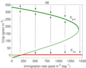
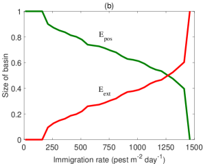
Figure 1: (a) Bifurcation diagram showing the equilibria $E_{\text{pos}}$ and $E_{\text{ext}}$ as a function of immigration of susceptible pests $A$. Solid curves denote stable equilibria while dotted curves denote unstable equilibria. (b) Size of basin of the equilibria $E_{\text{pos}}$ and $E_{\text{ext}}$ as a function of immigration of susceptible pests $A$. The extinction equilibria $E_{\text{ext}}$ attracts more and more of the state space as $A$ increases.

Typically, the system behave in a way that is shown by the trajectories in Fig. 2. The crop population will start growing slowly, followed by a rapid increase due to the logistic growth assumption. As the crop biomass is small it grows slowly, and a small perturbation may cause it to stay small during a long time interval, perhaps too long in order to get a good yield at the end of the growth season. If immigration is relatively high, a perturbation may also result in that the crop dies due to the attracting extinction equilibria $E_{\text{ext}}$. These facts motivate our efficacy measure half-biomass time introduced in Section 4. From Fig. 2a-c we can also see that as immigration of susceptible pests increases, then the disease spreads in the pest population so that the infected pests biomass $P_{I}$, rather than susceptible pests $P_{S}$, increases. When crop biomass is small, this can be understood by perturbing off the expression of the extinction equilibrium in (2.4). In particular, observe the term $A/d_{I}$ in the expression for $P_{I}$.

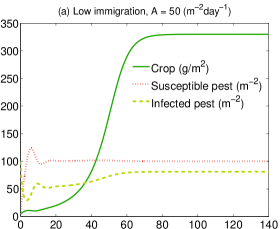
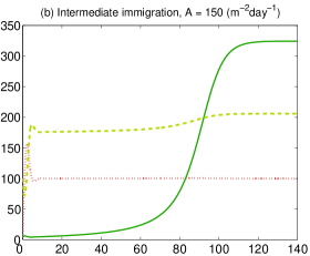
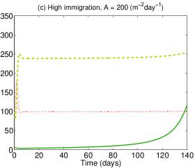
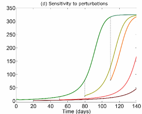
Figure 2: (a)-(c): Trajectories of crop (green, solid), susceptible pests (red, dotted) and infected pests (yellow, dashed). The soybean crop biomass increases rapidly at near half its equilibrium value. With higher immigration rate of susceptible pests, the rapid increase comes later in the season. In panel (c) it is delayed beyond the end of the season. (d): The final crop biomass is sensitive to perturbations in the beginning of the season when the crop biomass is small and grows slowly. Trajectory of crop biomass without perturbation (green). Trajectories of crop biomass with a sudden reduction to 1/4 of its amount at time 110 (yellow), 80 (orange), 50 (red) and 20 (dark red). Initial amount of infected pests is set to $P_{I}(0)=100$ g/m² and the immigration rate of susceptible pests is $A=150$.

As the system (2.1)–(2.3) is based on a predator-prey model of Rosenzweig-MacArthur type, one may expect it to have limit cycles in some cases. However, the extensive simulations of the basin of attraction presented in Fig. 1b indicate no attracting cycles. In Section 5.4 we consider robustness of our results with respect to variations in the parameter values, and these simulations also agree that the above equilibria remain the only attractors.

3.  Control strategies

Next, we introduce and give a precise definition of the control strategies that we consider for the release of infected individuals. We chose our class of control strategies for conceptual simplicity, though as we will show these strategies are capable of achieving near-optimal profits. Before describing the control strategies, we briefly note that the sample model in (2.1)-(2.3) considers only the number of pests as well as biomass of crop, no spatial dependence is involved. Consequently, we do not discuss practical methods for release of the infected pests in order to efficiently and inexpesively distribute them evenly across the field.

Among the simple control strategies, we first consider releasing infected pests only once, at the beginning of the season. We call this strategy one-off control. This simple strategy has one control variable, the total amount of released infected pests $\widetilde{P}_{I}$, and is specified by the initial amount of infected pests as

$$P_{I}(0)\,=\,\widetilde{P}_{I}.$$

We next consider periodic control in which we assume that the same amount of infected pests are released the first day of each week throughout the growing season. Since the growth of the crop biomass is most sensitive to perturbations in the beginning of the season, we always assume that the first release happens at the first day of the season. The first release is thus implemented by setting the initial amount of infected pests, $P_{I}(0)$. Then the same amount of infected pests is released the first day of any following week, ending with week $N$, where $N=1,2,3,\dots$. Thus, $N=1$ corresponds to one-off control. The periodic control strategy involves two control variables, the number of weeks $N$ where an impulse of infected pests is released, and the total amount of released infected pests $\widetilde{P}_{I}$. In particular, the implementation of periodic control can formally be written, for $N=2,3,4,\dots$, as

$$P_{I}(0)\,=\,\frac{\widetilde{P}_{I}}{N}\quad\text{and}\quad P_{I}(s)\,\to\,P_{I}(s)\,+\,\frac{\widetilde{P}_{I}}{N},$$

where $s=\{7,14,\dots 7(N-1)\}$.

4.  Dual-objective approach

We here define our measures of profit and efficacy, after which we describe the concept of Pareto efficiency used for dual-objective optimization.

Besides trying to optimize profit we also consider maximizing efficacy, i.e. minimizing sensitivity to perturbations on the profit. We will now define our profit function, our measure of efficacy, i.e. half-biomass time, and also recall the economic concept of Pareto efficiency, which we will use to trade-off between the two objectives profit and efficacy.

4.1.   Profit measure

To determine a profit function, we first assume that yield is proportional to crop biomass and, without loss of generality, that the constant of proportionality is 1. If $p_{\text{crop}}$ is the market price for the crop, then the revenue is given by $p_{\text{crop}}\,C(t_{\text{season}})$ where $t_{\text{season}}$ is the time at the end of the growth season. We also assume that the total cost is given by $p_{\text{fixed}}\,+\,p_{\text{infected}}\,\widetilde{P}_{I}\,+\,p_{\text{labour}}\,N$, where $p_{\text{fixed}}$ represents annually-recurring costs for seed, sowing, fertilizer, irrigation, pest monitoring, taxes, etc. that remain fixed within a single growth season; $p_{\text{infected}}$ is the price of infected pests; and $p_{\text{labour}}$ is cost for work needed to place a burst of infected pests in the field. Hence, the profit is given by

$$\textrm{Profit}\,=\,p_{\text{crop}}\,C(t_{\text{season}})\,-\,p_{\text{fixed}}\,-\,p_{\text{infected}}\,\widetilde{P}_{I}\,-\,p_{\text{labour}}\,N.$$ (4.1)

4.2.   Efficacy measure

To construct a measure of efficacy on the final crop biomass we first consider the typical behavior of trajectories. Figure 2 shows that, starting from a small initial crop biomass of 5 g/m², then crop grows slowly in the beginning of the season followed by a rapid increase starting at approximately 50 g/m². In particular, when crop biomass is small, then from (2.1) we see that $dC/dt\approx rC$ and so the relative (to biomass) growth rate is constant. Low profit results when the rapid increase in crop biomass takes place too late in the season. Hence, it is important that the period of fast growing crop biomass is within the growth season, as it is in Figs. 2a and b, but not in c. As Fig. 2d shows, the location of the rapid increase, and hence the final crop biomass, is sensitive to perturbations in the beginning of the season when the crop biomass is small and grows slowly. For relatively high immigration rates a perturbation on a small crop biomass may even cause the crop to go extinct because of the attraction from the extinction equilibrium, see Section 2.2. Hence, it is important to ensure that the crop comes away quickly from very small biomasses. Based on these observations, we chose to measure efficacy with half-biomass time, which we define as the time needed for the crop biomass to grow from its initial state to half of the equilibrium crop biomass. This equilibrium may be thought of as an expected value of the final crop biomass. The higher the half-biomass time is, the larger is the risk for the farmer to obtain a small (or zero) final crop biomass and hence a small (or negative) profit.

4.3.   Pareto efficiency

A control strategy is said to be Pareto efficient if any change in the control strategy will make either the profit or the efficacy worse. The Pareto front is defined as the set of all Pareto-efficient strategies. Hence, the Pareto front consist of the “best” strategies and the choice of strategy on this front depends on the desired trade-off between the two objectives. For further information on Pareto efficiency and dual-objective optimization, we recommend an introductory textbook such as Karpagam (1999).

5.  Results

Having introduced our modeling framework, we now demonstrate how to find preferable control strategies. First, we conclude that only a small reduction in profit allows for efficacious control strategies. Second, we show that one-off control strategies are sufficient when immigration rates of susceptible pests are low to intermediate, while periodic control strategies are recommended for high immigration rates. Finally, we conclude that the determined control strategies are not far from optimal in terms of profit, despite their simplicity. All simulations shown in Sections 5.1, 5.2 and 5.4 are performed using MATLABs ODE-solver ode45, while in Section 5.3 we used in addition the optimization software TOMLAB (Holmstrom, 1999).

5.1.   A small reduction in profit allows efficacious control strategies

Figure 3a-c shows different one-off and periodic control strategies for low, intermediate and high immigration of susceptible pests. In each panel, different curves correspond to different $N$, starting with one-off control, i.e. $N=1$ (green), and continuing with periodic controls for $N=2,3,4,\dots$ (black). Each point on these curves corresponds to a positive value of the released infected pests $\widetilde{P}_{I}$. Using Fig. 3a-c, we can find control strategies that give a profit close to optimal, in the sense of one-off and periodic control strategies, and which are simultaneously efficacious in the sense of having a short half-biomass time. This is possible since the slope of the Pareto front, in the sense of one-off and periodic control strategies, (light green curve) is small near the maximum profit of the front, in particular for low to intermediate immigration rates. We recommend such Pareto-efficient strategies in place of optimizing only profit, to obtain more stable outcomes.

In Table LABEL:tab:one, we specify in detail four representative strategies on the Pareto front. These strategies are marked with circles in Fig. 3a-c. All four strategies have a half-biomass time of less than 80 and profit not far from the highest that can be achieved for any strategy of the same type. Depending on how one wishes to trade off between profit and efficacy, other strategies on the Pareto front with higher or lower efficacy can naturally also be considered.

5.2.   One-off control strategies are sufficient for low to intermediate immigration while periodic control is preferable for high immigration

To find the type of preferable control strategies for different immigration rates of susceptible pests, we assume, as a rule of thumb, that the farmer wants to keep the half-biomass time below 80. Further improvements in efficacy will be chosen only if the slope of the Pareto-front is very small near half-biomass time 80, so that efficacy can be substantially improved to the cost of hardly no profit.

From Fig. 3a-c we can conclude that one-off control strategies are preferable for low to intermediate immigration rates, as such strategies can easily push the half-biomass time below 60 for low immigration and below 80 for intermediate immigration. For high immigration rates, we recommend periodic control with either two or three ($N=2$ or $N=3$) releases of infected pests. This is because one-off control cannot achieve sufficiently small half-biomass time in this case, see Fig. 3c. In particular, in a field with high immigration, using periodic control in place of one-off control can result in the half-biomass time being reduced by $25\%$ without reducing the profit. This is a natural and expected result: If the immigration of susceptible pests is high, then it is not enough to “push down” the pest biomass only in the beginning of the season, a more continuous maintenance, such as periodic control, is needed.

Table 2: Representative pest-control strategies.

Immigration, $A$	Profit	Half-biomass time	Released infected	Number of
(m-2 day-1)	($\$$ m-2)	(days)	pests, $\widetilde{P}_{I}$ (m-2)	pest bursts, $N$
$50$	0.132	53	64	1 (one-off)
$150$	0.126	72	256	1 (one-off)
$250$	0.089	79	1700	2 (periodic)
$250$	0.089	79	1450	3 (periodic)

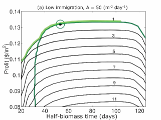
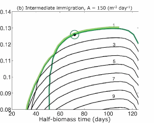
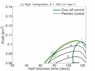
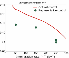
Figure 3: Pareto-efficient control strategies allow safe controls to a small cost in profit. The circles indicate representative control strategies on the Pareto front (light green curve). In each subfigure, different curves correspond to different $N$, starting with one-off control (green), and continuing with periodic controls for $N=2,3,4,\dots$ (black). Each point on these curves corresponds to a positive value of the released infected pests $\widetilde{P}_{I}$. Panels (a) and (b): For low to intermediate immigration, we recommend one-off controls, while for high immigration (c) periodic control is better and we recommend either two or three bursts ($N=2$ or $N=3$). Note that at the center of the circle in panel (c) the periodic control with two bursts ($N=2$) coincides with the periodic control with three bursts ($N=3$). (d): The representative control strategies are not far from optimal in the sense of profit. The optimal profit obtained by running the software TOMLAB, maximizing only profit, is given by the red curve. The profit of the representative control strategies is marked with green balls. In panel (d), all results are without cost for labour, i.e. $p_{\text{labour}}=0$.

5.3.   The determined control strategies are not far from optimal in terms of profit

To compare the representative control strategies in Table LABEL:tab:one to the optimal profit, when considering profit as the only target under optimization, we determined the best possible profit using the software TOMLAB (Holmstrom, 1999). Unlike the control strategies we have considered, this optimal control strategy can take any form and may be very hard to implement in practice. To compare the profit achieved through applying this optimal control strategy with those of our representative control strategies, we assume in this section that the labour cost for placing infected pests in the field is zero, i.e. $p_{\text{labour}}=0$. This assumption is necessitated by the fact that the determined optimal control strategy may require continuous release of infected individuals. By making this assumption, we thus achieve a situation in which the difference in profit between the two strategies should be largest.

Figure 3d shows the profit of the representative control strategies given in Table LABEL:tab:one (with $p_{\text{labour}}=0$) together with the optimal profit obtained by TOMLAB. We conclude that the profit of the representative control strategies are not far from the optimal profit in the whole range of immigration rate. In particular, the representative control strategies yield more than $85\%$ of the optimal profit. We remark that the gap between the optimal profit and the representative control strategies would decrease further when adding any reasonable labour cost to both controls. We have also observed, not surprisingly, that the trajectories for crop resulting from the optimal control strategies obtained by simulations in TOMLAB have a large half-biomass time. Therefore, they are sensitive to perturbations which in turn clearly yields an additional cost.

5.4.   Robustness

Consequences of variations in the price parameters can be understood from the profit function (4.1). In particular, increasing (decreasing) fixed costs $p_{\text{fixed}}$ will only lower (lift) all the curves in Fig. 3, and therefore our results are robust with variations in $p_{\text{fixed}}$. Increasing the price of placing infected pests in the field ($p_{\text{labour}}$) will be in favour of controls with few pest bursts such as one-off control ($N=1$). To understand the magnitude of this dependence we note from the profit function (4.1) that increasing (decreasing) $p_{\text{labour}}$ will lower (lift) the curves with $N\times$ the increase (decrease), where $N$ is the number of pest bursts.

We proceed by investigating robustness of our results by varying values of crop intrinsic growth rate $r$, contact rate $\beta$ as well as immigration of susceptible pests $A$. Figures 4a-c show regions where the recommended control is one-off control, periodic control and where it is impossible to obtain a positive profit. To find a border between recommending one-off or periodic control, we use here the following rule of thumb: We recommend to use periodic control, in place of one-off control, if the half-biomass time thereby can be reduced by at least $20\%$ without loosing more than $20\%$ of the best profit resulting from the one-off controls. Figures 4a-c are produced by examination of numerous figures of the same type as Fig. 3a-c. Besides results illustrated in Figs. 4a-c, we concluded from these simulations that the shape of the curves are rather stable. This means that our conclusion that a small reduction in profit allows efficacious control strategies is robust. Moreover, our conclusion that one-off control strategies are sufficient for (relatively) low to intermediate immigration holds whenever $r>0.4$ and $\beta>0.007$. In addition, the later conclusion can be extended as: one-off control strategies are sufficient for relatively low to intermediate immigration, as well as for relatively high contact rate and relatively high crop intrinsic growth rate.

The simulations in this section also verifies the natural facts that crop growth will increase in $r$, $\beta$ and decrease in $A$.

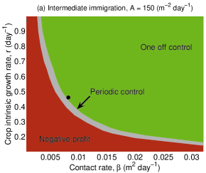
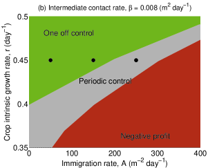
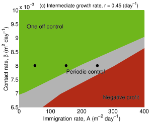
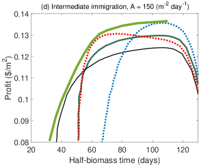
Figure 4: (a)-(c) Regions where the recommended control is one-off control (green), periodic control (grey) and where it is impossible to obtain a positive profit (red). The black dots represent parameter values used in Fig. 3. In each subfigure, 100 different parameter combinations, equally distributed over the presented area, have been tested. (a) Immigration rate $A=150$ is fixed while crop intrinsic growth rate $r$ and contact rate $\beta$ are varied. (b) Contact rate $\beta=0.008$ is fixed while crop intrinsic growth rate $r$ and immigration rate $A$ are varied. (c) Crop intrinsic growth rate $r=0.45$ is fixed while contact rate $\beta$ and immigration rate $A$ are varied. (d) Profit and half-biomass time when allowing for combinations of periodic controls and one-off controls in the setting of intermediate immigration $A=150$. The light-green curve represents the Pareto front corresponding to “all possible” combined control strategies. One-off control (dark-green), periodic control with $N=2$ and $\tau=7$ (black), periodic control with $N=2$ and $\tau=137$ (red, dotted), and combined one-off and periodic control consisting of one impulse $\widetilde{P}_{\text{one-off}}$ at time 0 and another impulse $\widetilde{P}_{\text{periodic}}$ at time 137 with $\widetilde{P}_{\text{one-off}}=0.1\widetilde{P}_{\text{periodic}}$ (blue, dotted).

6.  Discussion

We have considered biological control of agricultural pests. Using a dual-objective approach and the economic concept of Pareto efficiency, we have determined one-off and periodic control strategies that are stable to perturbations and simultaneously nearly optimal in terms of profit. Our optimization approach as well as our measure of efficacy are general and can be applied to effectively any crop-pest-pathogen system. Depending on the immigration rate of pests from nearby fields, we recommend either one-off control, with entomopathogens released only once in the beginning of the growing season, or periodic control, with entomopathogens released at periodic intervals. Surprisingly, as we showed in Section 5.3, these two conceptually simple pest-control strategies come close to the best that can be achieved, even when allowing for complicated continuous-release strategies.

The threshold for the immigration rate at which one should switch from one-off control to periodic control as well as the other control parameters can be determined through our approach after a model has been selected and parameterized for the system of interest. We also believe that it should be possible to determine reasonable values for the control parameters through controlled field experiments, or even individual experimentation. Future work may aim to overcome the problem of parametrization by deriving even more general insights, such as adaptive rules that relate the timing of release or the released quantity to observed changes in the crop and pest population.

When defining the periodic control strategies in Section 3, we assumed that the same amount of pests is released once a week. This assumption should be considered more as an example than a rule. In fact, the efficacy of the periodic control will only be marginally affected by smaller changes in the length of this time interval. The costs associated with the periodic control does, however, strongly depend on the price of placing the infected pests in the field ($p_{\text{labour}}$). A lower price will make the controls that releases more often (higher $N$) better. Moreover, a natural extension of the periodic controls tested here would be to allow for the combination of one-off control and periodic control. We have seen that one-off control performs well in most tested cases, and therefore we believe in releasing larger amounts of pests at impulses in the beginning of the growth season, and smaller amounts later during the season. We will further discuss this below.

We have considered dual-objective optimization which accounts for both efficacy and profit. The fundamental drawback with optimizing profit alone is that the resulting crop trajectory may behave similar to the trajectory for crop biomass given in Fig. 2b. Even worse, the increase in crop abundance may come closer to the end of the season so that a small perturbation during the growth season may pass it beyond the end of the season, as the trajectories of crop in Fig. 2c and d. Hence, instead of optimizing only profit, farmers should consider a trade-off between profit and some measure of efficacy (sensitivity to perturbations). To exclude growth patterns that are very sensitive to perturbations and hence implies a high risk for farmers, we introduced in Section 4 a measure of efficacy, the half-biomass time, and applied a dual-objective approach through Pareto efficiency.

Our measure of efficacy, half-biomass time, is related to resilience, which is nowadays frequently used in ecology (Pimm and Lawton, 1977; Loreau and Behera, 1999; Petchey et al., 2002; Montoya et al., 2006; Loeuille, 2010; Valdovinos et al., 2010). Resilience can be measured as the reciprocal of the returntime of a trajectory to a stable equilibrium, perturbed from the same equilibrium. See Lundström et al. (2016, 2017) for definitions, discussions and applications of such nonlocal resilience measures. In essence, short half-biomass time corresponds to high resilience as it means that the crop is quickly able to approach an equilibrium state. We define half-biomass time based on typical growth patterns for crops in our model. However, a similar definition will apply to other models showing similar growth patterns, involving models where biomass is assumed to grow logistically. To stress the generality of our work, we note that the measure half-biomass time may be replaced by any other suitable measure of efficacy which can be defined for the model in question, and a similar analysis using Pareto-efficiency and simple control strategies can be carried out.

The study closest to ours is the effort by Cardoso et al. (2009) in understanding biological control of caterpillars (Anticarsia gematalis) by natural enemies such as wasps and spiders. Similar to us, these authors use a dual-objective approach and use the economic concept of Pareto efficiency. In their case, the two objectives are measures of the number of prey (the pest) and the number of predators (the natural enemy of the pest) which are released. Like us, these authors aim to derive more practical pest-control strategies by moving away from continuous-release strategies towards release at specified time points, so-called impulsive release (Tang et al., 2005; Zhang et al., 2007). Apart from the different choice of study system, a few additional differences are worth noting: First, Cardoso et al. (2009) do not compare the impulsive-control strategies that they derive with simple one-off control and periodic-control strategies as considered here. Second, whereas we develop and motivate a non-linear measure of pest-control efficacy, Cardoso et al. (2009) uses a measure of the number of released natural enemies as their second objective. Third, we explicitly consider the dynamics of the crop and move beyond the traditional Lotka-Volterra framework by incorporating functional responses. Interestingly, the optimal strategies presented in Figs. 3-5 of Cardoso et al. (2009) have a clear resemblance to a periodic control except at the beginning and the end of season. Based on this observation and our own results, we conjecture that effective strategies of biological pest control can be obtained by combining one-off control and periodic control. Figure 4d shows the Pareto-front for profit and half-biomass time when allowing for such combinations in the setting of intermediate immigration $A=150$. In particular, the combined control has four control variables; the amount of released pests in the beginning of the season ($\widetilde{P}_{\text{one-off}}$), the total amount of released pests during the following periodic control ($\widetilde{P}_{\text{periodic}}$), the number of days between pest impulses ($\tau$) and the total number of impulses (${N}$). By comparing Fig. 3b with Fig. 4d we conclude that the Pareto front is slightly higher in Fig. 4d. Thus, allowing for combinations of periodic controls and one-off controls opens for slightly more efficient control strategies. This is expected since such approach allows for more degrees of freedom and can therefore better meet the populations need of pest control. Note, however, that we do not obtain a substantially better result. Moreover, the dotted curves in Fig. 4d, which reaches near Pareto optimality, consists of strategies with only two impulses ($N=2$), the first at the beginning of the season and the second near the end of the season. Hence, simple strategies performs well also when allowing for combinations of one-off control and periodic control.

As noted in this paper, several studies in applied mathematics have aimed to determine optimal strategies of biological pest control. These studies draw upon and synthesize a rich scientific heritage of mathematical modeling in ecology, dynamical systems theory, and optimal control theory. The crowning achievement is the ability to determine the optimal timing for releasing natural enemies across a range of pest-enemy systems. This accomplishment will, however, be of limited value if insights are not distilled and results disseminated in a form that is useful for the agricultural community. Our aim with this paper has been to demonstrate how practically useful pest-control strategies can be determined from mathematical models of crop-pest-enemy interactions. While we have arguably not succeeded in bridging the full width of the gulf that currently exist between mathematical theory and practical applications, we expect this gulf to shrink as future authors continue our effort to uncover practically useful strategies of biological pest control.

Acknowledgement. The work of HZ was supported by the Swedish Research Council, the National Natural Science Foundation of China, Grant ID 11201187 and the Scientific Research Foundation for the Returned Overseas Chinese Scholars and the China Scholarship Council. The authors thank Daniel Simpson for useful discussions and comments.

References

- (1)
- Ball et al. (2000) Ball R. A., Purcell L. C. and Vories E. D. 2000. Optimizing soybean plant population for a short-season production system in the southern USA. Crop Sci. 40, 757–764.
- Bhattacharyya and Bhattacharya (2006) Bhattacharyya S. and Bhattacharya D. K. 2006. Pest control through viral disease: mathematical modeling and analysis. J. Theo. Biol. 238, 177–197.
- Cardoso et al. (2009) Cardoso R. T. N., Cruz A. R. D., Wanner E. F. and Takahashi R. H. C. 2009. Multi-objective evolutionary optimization of biological pest control with impulsive dynamics in soybean crops. Bull. Math. Biol. 71, 1463–1481.
- Cherry et al. (1997) Cherry A. J., Parnell M. A., Grzywacz D. and Jones K. A. 1997. The optimization ofin VivoNuclear Polyhedrosis virus production in Spodoptera exempta (Walker) and Spodoptera exigua (Hübner). J. Invertebr. Pathol. 70, 50–58.
- Dale (2006) Dale G. 2006. Growing soybeans in northern Victoria. Agriculture Notes Dept. of Primary Industries, Victoria, AG1138.
- Dhaliwal et al. (2010) Dhaliwal G. S., Vikas J. and Dhawan A. K. 2010. Insect pest problems and crop losses: changing trends. Indian J. Ecol. 37, 1–7.
- Fuxa (2004) Fuxa J. R. 2004. Ecology of insect nucleopolyhedroviruses. Agric., Ecosyst. Environ. 103, 27–43.
- Getz and Gutierrez (1982) Getz W. M. and Gutierrez A. P. 1982. A perspective on systems analysis in crop production and insect pest management. Ann. Rev. Entomol. 27, 447–466.
- Grasman et al. (2001) Grasman J., Van Herwaarden O. A., Hemerik L. and Van Lenteren J. C. 2001. A two-component model of host-parasitoid interactions: determination of the size of inundative releases of parasitoids in biological pest control. Math. Biosci. 169, 207–216.
- Hethcote (2000) Hethcote H. W. 2000. The mathematics of infectious diseases SIAM review 42, 599–653.
- Holmstrom (1999) Holmstrom K. 1999. The TOMLAB optimization environment in Matlab. Adv. Model. Optim. 1, 47–69.
- Karpagam (1999) Karpagam M. 1999. Environmental economics: a textbook. Sterling Publishers Pvt. Ltd.
- Khooharo et al. (2008) Khooharo A. A., Memon R. A. and Lakho M. H. 2008. An assessment of farmers’ level of knowledge about proper usage of pesticides in Sindh Province of Pakistan. Sarhad J. Agric. (Pakistan).
- Komatsu et al. (2004) Komatsu K., Okuda S., Takahashi M. and Matsunaga R. 2004. Antibiotic effect of insect-resistant soybean on common cutworm (Spodoptera litura) and its inheritance. Breed. Sci. 54, 27–32.
- Lacey et al. (2001) Lacey L. A., Frutos R., Kaya H. K. and Vail P. 2001. Insect pathogen as biological control agents; Do they have a future? Biol. Control 21, 230–248.
- Li et al. (2010) Li S., Xiong Z., Wang X. 2010. The study of a predator-prey system with group defense and impulsive control strategy Appl. Math. Model. 34, 2546–2561.
- Liao et al (2016) Liao Z. H., Kuo T. C., Shih C. W., Tuan S. J., Kao Y. H., Huang R. N. 2016. Effect of juvenile hormone and pyriproxyfen treatments on the production of Spodoptera litura nuclear polyhedrosis virus. Entomologia Experimentalis et Applicata, 161, 112–120.
- Liu et al. (2015) Liu X., Rahman T., Song C., Su B., Yang F., Yong T., Wua Y, Zhange C, Yanga W. 2017. Changes in light environment, morphology, growth and yield of soybean in maize-soybean intercropping systems. Field Crops Research, 200, 38–46.
- Loeuille (2010) Loeuille N. 2010. Influence of Evolution on the Stability of Ecological Communities. Ecol. Lett. 13, 1536–1545.
- Loreau and Behera (1999) Loreau M., Behera N. 1999. Phenotypic Diversity and Stability of Ecosystem Processes. Theor. Popul. Biol. 56, 29–47.
- Lundström (2017) Lundström N. L. P. 2017. How to find simple nonlocal stability and resilience measures. arXiv preprint.
- Lundström and Aidanpää (2007) Lundström, N. L. P., Aidanpää, J-O. 2007. Dynamic consequences of electromagnetic pull due to deviations in generator shape. Journal of Sound and Vibration 301, 207–225.
- Lundström et al. (2016) Lundström N. L. P., Loeuille N., Meng X., Bodin M., Brännström Å. 2016. Meeting yield and conservation objectives by balancing harvesting of juveniles and adults. preprint.
- McCallum et al. (2001) McCallum H., Barlow N. and Hone J. 2001. How should pathogen transmission be modelled? Trends Ecol. Evol. 16, 295–300.
- Montoya et al. (2006) Montoya J. M., Pimm S. L. and Sole R. V. 2006. Ecological Networks and Their Fragility. Nature 442, 259–264.
- O’Reilly and Miller (2006) O’Reilly D. R. and Miller, L. K. 1989. A baculovirus blocks insect molting by producing ecdysteroid UDP-glucosyl transferase. Science 245, 1110–1112.
- Petchey et al. (2002) Petchey O. L., Casey T., Jiang L., McPhearson P. T. and Price, J. 2002. Species richness, environmental fluctuations, and temporal change in total community biomass. Oikos 99, 231–240.
- Pimm and Lawton (1977) Pimm S. L. and Lawton J. H. 1977. Number of Trophic Levels in Ecological Communities. Nature 268, 329–331.
- Rafikov et al. (2008) Rafikov M., Balthazar J. M. and von Bremen H. F. 1993. Mathematical modeling and control of population systems: applications in biological pest control. Appl. Math. Comput. 200, 557–573.
- Rosenzweig and MacArthur (1963) Rosenzweig M. L. and MacArthur R. H. 1963. Graphical representation and stability conditions of predator-prey interactions Am. Nat., 209–223.
- Ruiz-Nogueira et al. (2001) Ruiz-Nogueira B., Boote K. J., and Sau F. 2001. Calibration and use of CROPGRO-soybean model for improving soybean management under rainfed conditions. Agricultural Systems 68, 151–173.
- Tang et al. (2005) Tang S., Yanni X., Lansun C. and R. Cheke R. A. 1993. Integrated pest management models and their dynamical behaviour. Bull. Math. Biol. 67, 115–135.
- Valdovinos et al. (2010) Valdovinos F. S., Ramos-Jiliberto R., Garay-Narváez L., Urbani P. and Dunne J. A. 2010. Consequences of adaptive behaviour for the structure and dynamics of food webs. Ecol. Lett. 13, 1546–1559.
- Xiao and Van Den Bosch (2003) Xiao Y. and Van Den Bosch F. 2003. The dynamic of an eco-epidemic model with biological control. Ecol. Model. 168, 203–214.
- Yadav (2010) Yadav S. K. 2010. Pesticide applications-threat to ecosystems. J. Hum. Ecol. 32, 37–45.
- Zhang et al. (2007) Zhang H., Jiao J. and Lansun C. 2010. Pest management through continuous and impulsive control strategies. Biosystems 90, 350–361.
- Zhang and Georgescu (2015) Zhang H. and Georgescu P. 2015. The influence of the multiplicity of infection upon the dynamics of a crop-pest–pathogen model with defence mechanisms. Appl. Math. Model. 39, 2416–2435.