Compact stars with strongly coupled quark matter in a strong magnetic field

Abstract

Some time ago we have derived from the QCD Lagrangian an equation of state (EOS) for the cold quark matter, which can be considered an improved version of the MIT bag model EOS. Compared to the latter, our equation of state reaches higher values of the pressure at comparable baryon densities. This feature is due to perturbative corrections and also to non-perturbative effects. Later we applied this EOS to the study of compact stars, discussing the absolute stability of quark matter and computing the mass-radius relation for self-bound (strange) stars. We found maximum masses of the sequences with more than two solar masses, in agreement with the recent experimental observations. In the present work we include the magnetic field in the equation of state and study how it changes the stability conditions and the mass-radius curves.

I Introduction

In the theory of compact stars hebel ; emmi ; kojo ; fukojo ; drago ; fkv16 ; kfbv ; fkv14 there are still several key unanswered questions emmi . One of them is: “are there quark stars ?” This question has been around for decades and it has received a renewed attention after the appearance of new measurements of masses of astrophysical compact objects demorest ; anton ; vanker . These measurements suggest that stellar objetcs may have large masses, such as, for example, the pulsar PSR J1614-2230, with $(1.97\pm 0.04)\,M_{\bigodot}$ demorest or the pulsar PSR J0348+0432, with $(2.01\pm 0.04)\,M_{\bigodot}$ anton and perhaps the black widow pulsar PSR B1957+20, with a possible mass around $(2.4\pm 0.12)\,M_{\bigodot}$ vanker . In principle larger masses imply larger baryon densities in the core of the stars and we expect very dense hadronic matter to be in a quark gluon plasma (QGP) phase. On the other hand, from the theoretical point of view, most of the proposed equations of state for this cold QGP are too soft to be able to support such large masses.

The answer to the question above depends on the details of the equation of state of cold quark matter. According to most models, deconfined quark matter should be formed at baryon densities in the range $\rho_{B}=2\rho_{0}-5\rho_{0}$, where $\rho_{0}$ is the ordinary nuclear matter baryon density. Since at low temperatures and high baryon densities we can not rely on lattice QCD calculations, the quark matter equations of state must be derived from models. Many of them are based on the MIT bag model mit or on the Nambu-Jona-Lasinio (NJL) model nambu . In these models the gluon degrees of freedom do not appear explicitly. In the bag model they are contained in the bag constant and in the NJL they are integrated out giving origin to the four-quark terms. In more recent version of the NJL model kojo a bag-like term was introduced to represent the contribution of gluons to the pressure and energy density. At very high baryon densities there are constraints derived from perturbative QCD calculations fkv16 ; kfbv ; fkv14 ; pqcd . In Refs. we11 ; we111 we have developed a quark-gluon EOS, which was applied to the calculation of the structure of compact quark stars in Ref. we12 . Stars as heavy as $2\,M_{\bigodot}$ were found.

One important ingredient in the stellar structure calculation is the magnetic field. In magnetars, the strength of this field can reach values as large as $10^{18}\,G$. In theoretical calculations, magnetic field effects in astrophysical compact objects have been well studied magalera ; dpm3 .

In this work we extend the equation of state derived in Ref. we11 to the case where we have strong magnetic fields and check whether it is still able to support massive stars. Some steps along this direction have already been taken in Ref. we15 .

II Equation of state

The equation of state derived in we11 is based on a few assumptions. First we assume, as in the case of the hot QGP observed in heavy ion collisions, that the quarks and gluons in the cold QGP are deconfined but “strongly interacting”, forming a strongly interacting QGP (sQGP). This means that the coupling is not small and also that there are remaining non-perturbative interactions and gluon condensates. Of course, at very large densities (in the same way as at very high temperatures) the sQGP evolves to an ideal gas of non-interacting particles in a trivial vacuum. We split the gluon field into two components $G^{a\mu}={A}^{a\mu}+{\alpha}^{a\mu}$, where ${A}^{a\mu}$ (“soft” gluons) and ${\alpha}^{a\mu}$ (“hard”gluons) are the components of the field associated with low and high momentum respectively. The expectation values of ${A}^{a\mu}{A}^{a}_{\mu}$ and ${A}^{a\mu}{A}^{a}_{\mu}{A}^{b\nu}{A}^{b}_{\nu}$ are non-vanishing in a non-trivial vacuum and from them we obtain an effective gluon mass ($m_{G}$) and also a contribution (${\mathcal{B}}_{QCD}$) to the energy and to the pressure of the system similar to the one of the MIT bag model. Since the number of quarks is very large and their coupling to the gluons is not small, the high momentum levels of the gluon field will have large occupation numbers and hence the ${\alpha}^{a\mu}$ component of the field can be approximated by a classical field. This is the same mean field approximation very often applied to models of nuclear matter, such as the Walecka model.

In the next subsection we review the main formulas. For the details of the derivation we refer the reader to Ref. we11 .

II.1 Effective Lagrangian

Let us consider a system of deconfined quarks and gluons in a non-trivial vacuum immersed in an homogeneous magnetic field oriented along the Cartesian $z$ direction (we employ natural units $\hbar=c=k_{B}=1$ and metric given by $g_{\mu\nu}=\textrm{diag}(+,-,-,-)$) :

$$\vec{B}=B\hat{z}\hskip 34.14322pt\textrm{and}\hskip 34.14322ptA_{\mu}=(0,yB,0,0)$$ (1)

The Lagrangian is given by:

$${\mathcal{L}}={\mathcal{L}}_{QCD}\,+\,{\mathcal{L}}_{QED}$$ (2)

where ${\mathcal{L}}_{QCD}$, ${\mathcal{L}}_{QED}$ refer to the quarks and electrons which interact with the external magnetic field. The electrons are necessary to ensure the charge neutrality of the star, which will be enforced as in we12 . The Lagrangian (2) can be written as:

$${\mathcal{L}}=-{\frac{1}{4}}F^{a}_{\mu\nu}F^{a\mu\nu}+\sum_{f=u}^{d,s}\bar{\psi}_{i}^{f}\Big{[}i\gamma^{\mu}(\delta_{ij}\partial_{\mu}+i\delta_{ij}Q_{f}A_{\mu}-igT^{a}_{ij}G_{\mu}^{a})-\delta_{ij}m_{f}\Big{]}\psi_{j}^{f}$$

$$+\bar{\psi}_{i}^{e}\Big{[}i\gamma^{\mu}(\delta_{ij}\partial_{\mu}+i\delta_{ij}Q_{e}A_{\mu})-\delta_{ij}m_{e}\Big{]}\psi_{j}^{e}-{\frac{1}{16\pi}}F_{\mu\nu}F^{\mu\nu}$$ (3)

where the first and second lines represent the QCD and QED parts respectively. The summation in $f$ runs over the quark flavors: up ($u$), down ($d$) and strange ($s$), which have the following masses: $m_{u}=5\,MeV$, $m_{d}=7\,MeV$ and $m_{s}=150\,MeV$. The electron mass is $m_{e}=0.5\,MeV$. The respective charges are : $Q_{u}=2\,Q_{e}/3$, $Q_{d}=-\,Q_{e}/3$ and $Q_{s}=-\,Q_{e}/3$, where $Q_{e}$ is the absolute value of the electron charge. $T^{a}$ are the SU(3) generators, $f^{abc}$ are the SU(3) antisymmetric structure constants and the gluon field tensor is $F^{a\mu\nu}=\partial^{\mu}G^{a\nu}-\partial^{\nu}G^{a\mu}+gf^{abc}G^{b\mu}G^{c\nu}$. The electromagnetic Lagrangian term is $F^{\mu\nu}=\partial^{\mu}A^{\nu}-\partial^{\nu}A^{\mu}$, with $A^{\mu}$ given by (1). As mentioned above, we decompose the gluon field as in we11 ; we12 ; shakin ; shakinn :

$$G^{a\mu}={A}^{a\mu}+{\alpha}^{a\mu}$$

where ${A}^{a\mu}$ and ${\alpha}^{a\mu}$ are the soft and hard gluon components respectively. Repeating the same algebraic steps described in we11 we rewrite (3) as the following effective Lagrangian:

$$\mathcal{L}_{0}={\frac{{m_{G}}^{2}}{2}}{\alpha}^{a}_{0}{\alpha}^{a}_{0}-{\mathcal{B}}_{QCD}-{\frac{B^{2}}{8\pi}}+\bar{\psi}_{i}^{e}\Big{[}i\gamma^{\mu}(\delta_{ij}\partial_{\mu}+i\delta_{ij}Q_{e}A_{\mu})-\delta_{ij}m_{e}\Big{]}\psi_{j}^{e}$$

$$+\sum_{f=u}^{d,s}\bar{\psi}_{i}^{f}\Big{\{}i\gamma^{\mu}\Big{[}\delta_{ij}\partial_{\mu}+i\delta_{ij}Q_{f}A_{\mu}\Big{]}+g_{h}\gamma^{0}T^{a}_{ij}\alpha^{a}_{0}-\delta_{ij}m_{f}\Big{\}}\psi_{j}^{f}$$ (4)

The classical field $\alpha^{a}_{0}$ is the time component of ${\alpha}^{a\mu}$ and it comes from the mean field approximation ${\alpha}^{a}_{\mu}={\alpha}^{a}_{0}\delta_{\mu 0}$ we11 . The constant ${\mathcal{B}}_{QCD}$ is the “bag term” given by ${\mathcal{B}}_{QCD}\equiv 9{\,\phi_{0}}^{4}/136$ and ${m_{G}}$ is the dynamical gluon mass given by ${m_{G}}^{2}\equiv 9{\,\mu_{0}}^{2}/32$. The constant $\mu_{0}$ is an energy scale associated with $\langle A^{2}\rangle$, which is the gluon condensate of dimension two we11 :

$$\langle A^{2}\rangle\equiv\langle g_{s}^{2}{A}^{a\mu}{A}^{b\nu}\rangle=\langle g_{s}^{2}A^{2}\rangle=-{\frac{\delta^{ab}g^{\mu\nu}}{32}}{\mu_{0}}^{2}$$ (5)

Since $\langle g_{s}^{2}A^{2}\rangle$ $<0$ we always have ${m_{G}}^{2}$ $>0$. The constant $\phi_{0}$ is associated with $\langle F^{2}\rangle$, which is the gluon condensate of dimension four we11 :

$${\mathcal{B}}_{QCD}=b\phi_{0}^{4}=\langle\frac{1}{4}F^{a\mu\nu}F^{a}_{\mu\nu}\rangle={\frac{\pi^{2}}{g_{s}^{2}}}\langle{F}^{2}\rangle$$ (6)

In the expressions (4) and (5) we have two QCD coupling constants given by $g_{h}$ and $g_{s}$. The coupling $g_{h}$ is associated to the hard gluons, while $g_{s}$ is associated to the soft gluons as in we11 .

II.2 Equations of motion and Landau levels

The following equations of motion are derived from (4):

$$\Big{[}i\gamma^{\mu}\Big{(}\partial_{\mu}+iQ_{f}A_{\mu}\Big{)}+g_{h}\gamma^{0}T^{a}\alpha^{a}_{0}-m_{f}\Big{]}\psi^{f}=0$$ (7)

$$\Big{[}i\gamma^{\mu}\Big{(}\partial_{\mu}+iQ_{e}A_{\mu}\Big{)}-m_{e}\Big{]}\psi^{e}=0$$ (8)

$${m_{G}}^{2}{\alpha}^{a}_{0}=-g_{h}\sum_{f}\rho_{f}^{a}=-g_{h}\,\rho^{a}$$ (9)

where $\rho^{a}$ is the temporal component of the color vector current $j^{a\nu}$, given by:

$$j^{a0}=\rho^{a}=\sum_{f}{\bar{\psi}_{i}}^{f}\gamma^{0}T^{a}_{ij}\psi_{j}^{f}=\sum_{f}{{\psi}_{i}^{\dagger}}^{f}T^{a}_{ij}\psi_{j}^{f}$$ (10)

From the exact solution bacharia of the Dirac equation (7) with magnetic field and hard gluon terms, we have the following expression for the eigenvalues:

$$\Bigg{(}E_{\nu}^{f}+g_{h}\mathcal{A}\Bigg{)}^{2}=m_{f}^{2}+k_{z}^{2}+(2\nu+1)|Q_{f}|B-Q_{f}Bs$$ (11)

where $\nu=0,1,2,3,4,5\dots$ and $s=+1$ or $s=-1$, for the projection up or down of the spin states, respectively. The momentum component along the magnetic field direction is given by $k_{z}$. As in Ref. we11 the constant $\mathcal{A}$ in (11) is the “algebra valued” quantity, $\mathcal{A}=c^{\dagger}_{i}T^{a}_{ij}c_{j}\alpha_{0}^{a}$ (with the implicit summation over $i,j=1,2,3$ and $a=1,\dots,8$), where $c_{i}$ is a color vector, as explained in the Appendix. In Eq. (3) and in what follows, we do not include the interaction terms between the magnetic field and the fermion magnetic moments magspacks . This is because in Ref. dpm3 ; magmomentdaryel it was shown that for strange quark matter in $\beta-$ equilibrium in magnetic fields weaker than $10^{18}\,G$ the contribution of these terms can be neglected. More precisely, we will restrict our analysis to $B\leq 5\times 10^{17}\,G$.

Rescaling the single particle energy as $\tilde{E}_{\nu}^{f}\equiv E_{\nu}^{f}+g_{h}\mathcal{A}$ , we are able to rewrite (11) as:

$$\Big{(}\tilde{E}_{\nu}^{f}\Big{)}^{2}=m_{f}^{2}+k_{z}^{2}+\Big{[}2\nu+1-s\times sgn(Q_{f})\Big{]}|Q_{f}|B$$ (12)

where $Q_{f}=sgn(Q_{f})\times|Q_{f}|$. Defining $2\nu+1-s\times sgn(Q_{f})\equiv 2n$, (12) becomes:

$$\tilde{E}_{n}^{f(\pm)}=\pm\sqrt{m_{f}^{2}+k_{z}^{2}+2n|Q_{f}|B}$$ (13)

and $n$ denotes the $n^{th}$ Landau level. We note that, except for the rescaling in $\tilde{E}_{\nu}^{f}$, the equation above is the one usually found in the literature. Analogously, from the exact solution of (8) bacharia for the electron we have:

$$\Big{(}E_{\nu}^{e}\Big{)}^{2}=m_{e}^{2}+k_{z}^{2}+(2\nu+1)|Q_{e}|B-Q_{e}Bs$$ (14)

and considering $2\nu+1-s\times sgn(Q_{e})=2n$ we find the energy for the $n^{th}$ Landau level:

$$E_{n}^{e(\pm)}=\pm\sqrt{m_{e}^{2}+k_{z}^{2}+2n|Q_{e}|B}$$ (15)

II.3 Energy density and pressure

To obtain our EOS we follow the thermodynamical calculations as performed in dpm3 ; furn ; wenpa . The details are in the Appendix, where we also show the baryon density calculation. The quark density at zero temperature is given by:

$$\rho=\sum_{f=u}^{d,s}\,{\frac{|Q_{f}|B}{2\pi^{2}}}\,\sum_{n=0}^{n^{f}_{max}}3(2-\delta_{n0})\,k^{f}_{z,F}(n)$$ (16)

where $k^{f}_{z,F}(n)$ is the quark Fermi momentum given by:

$$k^{f}_{z,F}(n)=\sqrt{{\nu_{f}}^{2}-m_{f}^{2}-2n|Q_{f}|B}$$ (17)

The summation over the Landau levels is calculated on the condition that the expression under the square root in (17) is positive, i.e., ${\nu_{f}}^{2}\geq m_{f}^{2}+2n|Q_{f}|B$   dpm3 . Thus

$$n\leq n^{f}_{max}={\it{int}}\Bigg{[}\,{\frac{{\nu_{f}}^{2}-m_{f}^{2}}{2|Q_{f}|B}}\,\Bigg{]}$$ (18)

where ${\it{int}}[a]$ denotes the integer part of $a$. Analogously, for the electrons we have:

$$\rho_{e}={\frac{|Q_{e}|B}{2\pi^{2}}}\,\sum_{n=0}^{n^{e}_{max}}(2-\delta_{n0})\,k^{e}_{z,F}(n)$$ (19)

with

$$k^{e}_{z,F}=\sqrt{{\mu_{e}}^{2}-m_{e}^{2}-2n|Q_{e}|B}$$ (20)

and

$$n\leq n^{e}_{max}={\it{int}}\Bigg{[}\,{\frac{{\mu_{e}}^{2}-m_{e}^{2}}{2|Q_{e}|B}}\,\Bigg{]}$$ (21)

The energy density, the parallel pressure and the perpendicular pressure are:

$$\varepsilon={\frac{27}{16}}\,{\xi}^{2}{\rho_{B}}^{2}+{\mathcal{B}}_{QCD}+{\frac{B^{2}}{8\pi}}+{\frac{|Q_{e}|B}{2\pi^{2}}}\,\sum_{n=0}^{n^{e}_{max}}(2-\delta_{n0})\int_{0}^{k^{e}_{z,F}}dk_{z}\sqrt{m_{e}^{2}+k_{z}^{2}+2n|Q_{e}|B}$$

$$+\sum_{f=u}^{d,s}{\frac{|Q_{f}|B}{2\pi^{2}}}\,\sum_{n=0}^{n^{f}_{max}}3(2-\delta_{n0})\int_{0}^{k^{f}_{z,F}}dk_{z}\sqrt{m_{f}^{2}+k_{z}^{2}+2n|Q_{f}|B}$$ (22)

$$p_{\parallel}={\frac{27}{16}}\,{\xi}^{2}{\rho_{B}}^{2}-{\mathcal{B}}_{QCD}-{\frac{B^{2}}{8\pi}}+{\frac{|Q_{e}|B}{2\pi^{2}}}\,\sum_{n=0}^{n^{e}_{max}}(2-\delta_{n0})\int_{0}^{k^{e}_{z,F}}dk_{z}\,{\frac{{k_{z}}^{2}}{\sqrt{m_{e}^{2}+k_{z}^{2}+2n|Q_{e}|B}}}$$

$$+\sum_{f=u}^{d,s}{\frac{|Q_{f}|B}{2\pi^{2}}}\,\sum_{n=0}^{n^{f}_{max}}3(2-\delta_{n0})\int_{0}^{k^{f}_{z,F}}dk_{z}\,{\frac{{k_{z}}^{2}}{\sqrt{m_{f}^{2}+k_{z}^{2}+2n|Q_{f}|B}}}$$ (23)

$$p_{\perp}={\frac{27}{16}}\,{\xi}^{2}{\rho_{B}}^{2}-{\mathcal{B}}_{QCD}+{\frac{B^{2}}{8\pi}}+{\frac{|Q_{e}|^{2}B^{2}}{2\pi^{2}}}\,\sum_{n=0}^{n^{e}_{max}}(2-\delta_{n0})n\int_{0}^{k^{e}_{z,F}}{\frac{dk_{z}}{\sqrt{m_{e}^{2}+k_{z}^{2}+2n|Q_{e}|B}}}$$

$$+\sum_{f=u}^{d,s}{\frac{|Q_{f}|^{2}B^{2}}{2\pi^{2}}}\,\sum_{n=0}^{n^{f}_{max}}3(2-\delta_{n0})n\int_{0}^{k^{f}_{z,F}}{\frac{dk_{z}}{\sqrt{m_{f}^{2}+k_{z}^{2}+2n|Q_{f}|B}}}$$ (24)

where $\xi\equiv g_{h}/m_{G}$, as in we12 . Throughout this work we compute the values for the baryon density $\rho_{B}$ as multiples of the usual nuclear matter $\rho_{0}=0.17\,fm$.

We remember that when $\xi=0$ we recover the result of the MIT bag model. In this case we do not consider the electrons and just focus on the pure QCD matter, varying the baryon density from $1.3\,\rho_{0}$ to $4.8\,\rho_{0}$. The results are shown in Fig. 1 for the parallel and perpendicular pressures. We have chosen $\xi=0.002\,MeV^{-1}$, ${\mathcal{B}}_{QCD}=50\,MeV/fm^{3}$ and varied the magnetic field from zero to $B=5\times 10^{17}\,G$. As can be seen in the figure there are no causality violations (in which case we would have ${c_{s}}^{2}=\partial p/\partial\varepsilon>1$). The parallel pressure (Fig. 1a) decreases as the magnetic field increases, while the perpendicular pressure (Fig. 1b) increases with the magnetic field. Up to the considered maximum value of the magnetic field, the dependence of $p_{\parallel}$ and $p_{\perp}$ with $B$ is very mild. Moreover they are almost equal to each other. However at higher values of the magnetic field there is a rapid splitting between $p_{\parallel}$ and $p_{\perp}$, which is shown in Fig. 2. At $B=5\times 10^{17}\,G$ the difference between the two pressures is not yet very pronounced (less than 10 %) and the spherical symmetry can still be used to derive the standard Tolman-Oppenheimer-Volkov equations. The results shown in Fig. 2 are compatible with those shown in Fig. 1 of Ref. laura and also with those shown in Fig. 5 of Ref. dex-12 , where the quark matter was represented by slightly different versions of the MIT bag model equation of state. The main difference is that, while in these works the pressure anisotropy starts at $B\simeq 10^{18}$ G, in our calculations it starts earlier, at $B\simeq 10^{17}$ G. This happens because of the term proportional to ${\rho_{B}}^{2}$ appearing in the energy density (22) and in the pressure (23)-(24), which depends quadratically on $B$, as can be seen from (16). This term anticipates the high $B$ behavior of the pressure and the appearance of the pressure anisotropy.

At this point a remark is in order. As discussed in detail in dex-12 , there is a controversy in the literature concerning the existence or non-existence of pressure anisotropies. In early works (see the references quoted in dex-12 ) it was explicitly demonstrated that, in the presence of a background magnetic field, a Fermi-gas of spin-one-half particles possesses a pressure anisotropy. Later the calculations were revisited and the effects of the anomalous magnetic moment were included. It was concluded that the pressure anisotropy exists for both charged and uncharged particles, with and without anomalous magnetic moment. On the other hand, in Ref. bland and more recently in yako it was argued that, due to the presence of a non-vanishing magnetization one needed to additionally take into account the Lorentz force of the external magnetic field on the bound current densities, which would lead the system to isotropization. While this question is certainly very interesting we will stay on the safe side, avoid the region of very high $B$ and consider only values of the magnetic field where the pressure is isotropic. More precisely, in what follows we will compute the star masses up to $B=5\times 10^{17}\,G$ using the two different pressures and interpret the results as upper and lower limits of our calculations, regarding their difference as a theoretical error.

(a)

(b)

Figure 1: Dependence of the EOS on the magnetic field. (a) Parallel pressure. (b) Perpendicular pressure.

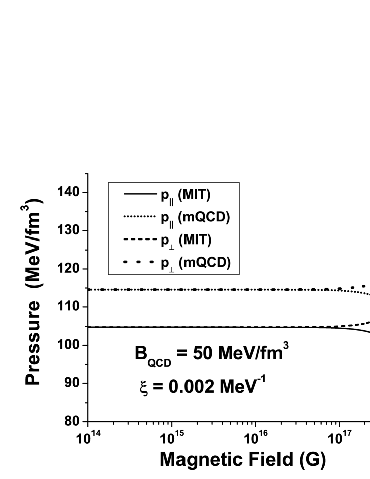
Figure 2: The splitting between the paralell and perpendicular pressures as a function of the magnetic field for mQCD and for the MIT bag model.

III Stability conditions

We wish to study stellar models with stable strange quark matter (described by the mQCD equation of state) and hence we will impose the stability conditions. The first condition is the existence of chemical equilibrium in the weak processes involving the quarks $u$, $d$, $s$ and electrons farhi ; glend :

$$u+e^{-}\rightarrow d+\nu_{e},\hskip 42.67912ptu+e^{-}\rightarrow s+\nu_{e},$$

$$d\rightarrow u+e^{-}+\bar{\nu}_{e},\hskip 42.67912pts\rightarrow u+e^{-}+\bar{\nu}_{e},\hskip 28.45274pt\textrm{and}\hskip 28.45274pts+u\rightarrow d+u.$$ (25)

which provides the following relations among the chemical potentials:

$$\nu_{d}=\nu_{s}\equiv\mu\hskip 28.45274pt\textrm{and}\hskip 28.45274pt\nu_{u}+\mu_{e}=\mu$$ (26)

The second condition is the global charge neutrality enforced by:

$${\frac{2}{3}}\rho_{u}={\frac{1}{3}}\rho_{d}+{\frac{1}{3}}\rho_{s}+\rho_{e},$$ (27)

The third condition is the baryon number conservation, which implies that we12 :

$$\rho_{B}={\frac{1}{3}}\rho={\frac{1}{3}}(\rho_{u}+\rho_{d}+\rho_{s})$$ (28)

The last condition is the requirement that the energy per baryon must be lower than the infinite baryonic matter defined in farhi and higher than the two flavor quark matter at the ground state farhi . We must impose that we12 :

$${\frac{\varepsilon}{\rho_{B}}}\bigg{|}_{(3\,\textrm{-flavor})}\,\,\,\,\,\leq\,\,934\,\,\mbox{MeV}\,\,\leq\,\,\,\,\,\frac{\varepsilon}{\rho_{B}}\bigg{|}_{(2\,\textrm{-flavor})}$$ (29)

We find numerically the values of $\xi$ and $\mathcal{B}_{QCD}$ which satisfy (26) to (29) simultaneously. Some examples of stability regions in the $\xi\,-\,\mathcal{B}_{QCD}$ parameter space are presented in Fig. 3, where the regions defined by the curves are the “stability windows” of $\xi$ as a function of $\mathcal{B}_{QCD}$. We observe that increasing the baryon density the window “shrinks”, i.e., the stability area becomes smaller and thinner. There is a maximum baryon density, $\rho_{B}\simeq 3.7\,\rho_{0}$, beyond which there is no stability window. This was expected and could be anticipated by looking at the first term of Eq. (22). When $\rho_{B}$ grows this term becomes dominant and the ratio $\varepsilon/\rho_{B}$ grows in such a way that it can no longer satisfy the left inequality in (29). The same reasoning applies to the value of the magnetic field. From (22) we can infer that there is a value of $B$, beyond which there will be no stability.

In Fig. 4 we show the diagram of stability as function of the magnetic field for the mQCD equation of state. From the figure we can observe that there is a maximum values of $\rho_{B}$ and of the field $B$, beyond which there is no stability.

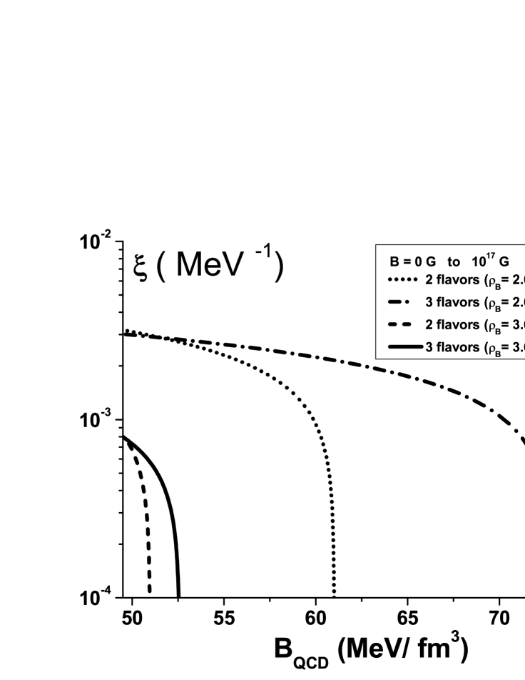
Figure 3: Stability windows defined by the conditions (26) to (29).

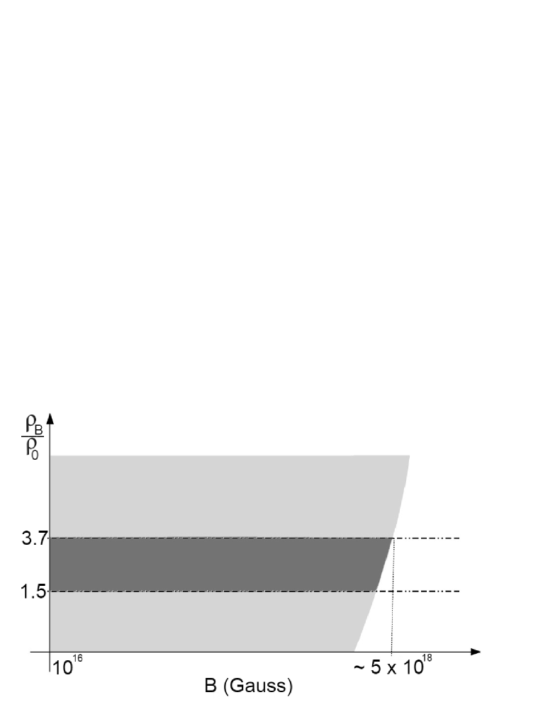
Figure 4: Stability diagram: baryon density ratio as function of magnetic field. The points in the light grey area satisfy the conditions (26), (27) and (28). Points in the dark grey area satisfy also the condition (29).

IV Stellar structure

As usual, to describe the structure of a static and non-rotating compact star, the Einstein equations are solved for the spherical, isotropic, static and general relativistic ideal fluid in hydrostatic equilibrium. Under these conditions, the solution of the Einstein equations provides the Tolman-Oppenheimer-Volkoff (TOV) equation for the pressure $p(r)$:

$$\frac{dp}{dr}=-\frac{G\epsilon(r)M(r)}{r^{2}}\left[1+\frac{p(r)}{\epsilon(r)}\right]\left[1+\frac{4\pi r^{3}p(r)}{M(r)}\right]\times\left[1-\frac{2GM(r)}{r}\right]^{-1},$$ (30)

where $G$ is the Newton gravitational constant. The mass $M(r)$ of the compact star is given by the mass continuity equation:

$$\frac{dM(r)}{dr}=4\pi r^{2}\epsilon(r).$$ (31)

In general, magnetic fields tend to deform a star and for larger magnetic fields, there will be a large deformation caused by changes in the metric inside the star. This aspect has been well studied in the literature, as for example, in tovsno . In these situations, where the magnetic fields are of the order of $10^{18}\,G$, the use of the spherically symmetric TOV equations to study the star structure is not appropriate. Therefore we will restrict our study to fields up to $5\times 10^{17}\,G$.

We solve numerically the coupled nonlinear equations (30) and (31) for $p(r)$ and $M(r)$, in order to obtain the mass-radius diagram. The possible magnetic field effects in the stellar structure come from the EOS. We consider the central energy density $\epsilon(r=0)=\epsilon_{c}$ and then we integrate both (30) and (31) from $r=0$ up to $r=R$ (stellar radius), where the pressure at the surface is zero: $p(r=R)=0$.

In Fig. 5 we present some solutions of the TOV equations and the resulting mass-radius diagrams. We fix $\mathcal{B}_{QCD}$, $\xi$ and $\rho_{B}$ respecting the stability windows and consider two values for the magnetic field. From the figure we observe that the mQCD model predicts larger masses than the MIT one and also that all values of the magnetic field, from zero to $5\times 10^{16}\,G$, yield the same mass-radius curves. In this range of $B$ values the parallel and perpendicular pressures are equal. One of main conclusions of Ref. we12 was that, with the EOS provided by mQCD, it was possible to have strange quark stars with two (or more) solar masses. The purpose of the calculations presented in Fig. 5 is to show that this remains true for strong magnetic fields.

In Fig. 6 we show how the mass-radius curves change when we keep the magnetic field constant and change $\mathcal{B}_{QCD}$ and $\xi$. We solve the equations (30) and (31) using the parallel and perpendicular pressures, given respectively by (23) and (24). As expected, smaller values of $\mathcal{B}_{QCD}$ imply higher pressure and higher masses, as we can see in Fig. 6a. A larger value of $\xi$ increases the pressure and the values of the obtained masses, as shown in Fig. 6b. These results are in qualitative agreement with those found in we12 at zero magnetic field. At $B=5\times 10^{17}$ G there is a visible difference between the results obtained with parallel and perpendicular pressures. This is the point where we stop our calculations and the difference between the results obtained with $p_{\parallel}$ and $p_{\perp}$ give an estimate of our theoretical error. However, if we insist on solving the TOV equations even for values of $B$ for which the pressure is anisotropic, we obtain the masses shown in Fig. 7. Comparing with Fig. 2, we observe that there is a direct correspondence between pressure and star mass. Under the same change of $B$ (from $10^{17}$ to $10^{18}$ Gauss) the pressures and masses change by a similar amount of $\simeq 20$ % or less.

Figure 5: Mass-radius diagrams. Two values of the magnetic fields with $\mathcal{B}_{QCD}$ and $\xi$ allowed by the stability conditions at $\rho_{B}=2.6\,\rho_{0}$. The largest masses are $2.05$ (mQCD) and $1.89$ (MIT). In these cases $p_{\parallel}=p_{\perp}$ which permits the use of TOV.

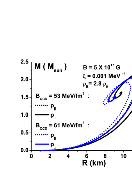
(a)

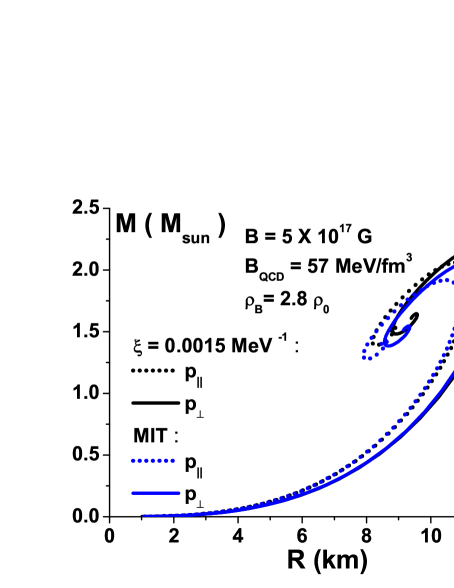
(b)

Figure 6: Mass-radius diagram for a fixed value of the magnetic field and the baryon density with $p_{\parallel}<p_{\perp}$. (a) Fixed $\xi$. For $\mathcal{B}_{QCD}=53\,MeV/fm^{3}$ the largest masses are $2.22$ and $2.04$ (along the dotted lines), calculated with the perpendicular and parallel pressures respectively. Analogously for $\mathcal{B}_{QCD}=61\,MeV/fm^{3}$ the largest masses are $2.06$ and $1.93$ (along the solid lines). (b) Fixed $\mathcal{B}_{QCD}$. For $\xi=0.0015\,MeV^{-1}$ the largest masses are $2.20$ and and $2.06$ (along the dotted lines), calculated with perpendicular and parallel pressures respectively. Analogously for MIT $(\xi=0\,MeV^{-1})$ the largest masses are $2.08$ and $1.92$ (along the solid lines).

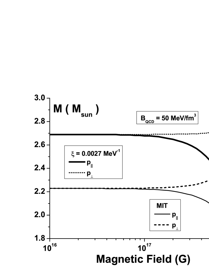
Figure 7: Effect of the pressure anisotropy on the star masses computed with the TOV equations. The chemical potentials obey the stability conditions (26), (27), (28) and (29), given by $\nu_{u}=300\,MeV$, $\nu_{d}=\nu_{s}=316.5\,MeV$ and $\mu_{e}=16.5\,MeV$ .

V Conclusions

We have evaluated the equation of state derived in Ref. we11 (which we call mQCD) at very large baryon densities, where deconfined quark matter should exist. In our model the ideal gas behavior is reached in the limit $\mathcal{B}_{QCD}\rightarrow 0$, $g_{h}\rightarrow 0$ and $m_{G}\rightarrow 0$ (respecting the condition $\xi=g_{h}/m_{G}\rightarrow 0$). In this limit we obtain the Stefan-Boltzmann (SB) equation of state. The results of Ref. fkv16 suggest that the SB limit is not yet reached at chemical potentials in the range $1\,\mbox{GeV}\leq\mu_{B}\leq 3\,\mbox{GeV}$ . In our model this means that the pressure is lowered (with respect to the SB value) because the quarks have non-zero masses or because of a non-vanishing gluon condensate or because of the two reasons combined.

We have introduced the magnetic field in the mQCD equation of state. We observe the splitting of the pressure into parallel, $p_{\parallel}$, and perpendicular, $p_{\perp}$, pressures. When $B$ increases, $p_{\perp}$ increases whereas $p_{\parallel}$ decreases. In our model this splitting starts to happen when $B\simeq 10^{17}$ G and it is a modest effect until $B\simeq 5\times 10^{17}$ G. Since larger pressures are essential to generate stars with larger masses, it is not clear a priori what is the effect of the magnetic field on the mass of the star. Moreover, increasing $B$ the stability window shrinks and from $B\simeq 5\times 10^{18}$ G on, we can not find any stable quark star. At these values the difference between $p_{\parallel}$ and $p_{\perp}$ is so large that we should no longer use the standard spherically symmetric TOV equations. Even though it was not possible to determine a clear trend of mass-radius curves with the magnetic field, we could find stars with more than two solar masses at $B\simeq 10^{17}\,G$. From this we can conclude that the heavy and magnetized stellar objects mentioned in the introduction can be, among other possibilities, quark stars.

To summarize: in our model the magnetic field does not generate any noticeable effect until $10^{17}$ G. From this point on, it generates a pressure anisotropy which precludes the use of the TOV equations. Moreover, it rapidly increases the energy density closing the stability window for this kind of strange quark matter.

VI Appendix

In this Appendix we present some details of the derivation of Eqs. (16), (22), (23) and (24).

VI.1 Baryon density

The $c_{j}$ is the quark color vector used in some textbooks grif :

$$c_{1}=\left(\begin{array}[]{c}1\\ 0\\ 0\end{array}\right)\hskip 8.5359pt\textrm{for red,}\hskip 5.69046ptc_{2}=\left(\begin{array}[]{c}0\\ 1\\ 0\end{array}\right)\hskip 8.5359pt\textrm{for blue,}\hskip 5.69046ptc_{3}=\left(\begin{array}[]{c}0\\ 0\\ 1\end{array}\right)\hskip 8.5359pt\textrm{for green}$$ (32)

From the above definitions it follows that $c^{\dagger}_{i}\delta_{ij}c_{j}=c^{\dagger}_{1}c_{1}+c^{\dagger}_{2}c_{2}+c^{\dagger}_{3}c_{3}=3$. For future purposes we will replace the above sum by the following average:

$$c^{\dagger}_{i}\delta_{ij}c_{j}\rightarrow{\frac{c^{\dagger}_{i}\delta_{ij}c_{j}}{(\textrm{number of quark colors})}}={\frac{c^{\dagger}_{1}c_{1}+c^{\dagger}_{2}c_{2}+c^{\dagger}_{3}c_{3}}{3}}=1$$ (33)

With the help of (32) we are able to calculate the relation between $\rho^{a}$ previously identified in (10) and the net quark density $\rho$. We perform the product $\rho^{a}\rho^{a}$ taking the average over the number of $SU(3)$ generators, which is $8$, as follows:

$$\rho^{a}\rho^{a}=\sum_{f}\rho_{f}^{a}\sum_{f^{\prime}}\rho_{f^{\prime}}^{a}\longrightarrow\langle\sum_{f}\rho_{f}^{a}\sum_{f^{\prime}}\rho_{f^{\prime}}^{a}\rangle={\frac{1}{8}}\sum_{f}\rho_{f}^{a}\sum_{f^{\prime}}\rho_{f^{\prime}}^{a}$$

$$={\frac{1}{8}}\sum_{f}({\psi}^{\dagger\,f}_{i}T^{a}_{ij}\psi^{f}_{j})\sum_{f^{\prime}}({\psi}^{\dagger\,f^{\prime}}_{k}T^{a}_{kl}\psi^{f^{\prime}}_{l})={\frac{1}{8}}\sum_{f}({c}^{\dagger}_{i}T^{a}_{ij}c_{j}){\psi}^{\dagger\,f}\psi^{f}\sum_{f^{\prime}}({c}^{\dagger}_{k}T^{a}_{kl}c_{l}){\psi}^{\dagger\,f^{\prime}}\psi^{f^{\prime}}$$

The result $({c}^{\dagger}_{i}T^{a}_{ij}c_{j})({c}^{\dagger}_{k}T^{a}_{kl}c_{l})=3$ is obtained from the Gell-Mann matrices and from the color vectors (32):

$$\rho^{a}\rho^{a}=\sum_{f}\rho_{f}^{a}\sum_{f^{\prime}}\rho_{f^{\prime}}^{a}={\frac{3}{8}}\sum_{f}({\psi}^{\dagger\,f}\psi^{f})\sum_{f^{\prime}}({\psi}^{\dagger\,f^{\prime}}\psi^{f^{\prime}})$$

As $\sum_{f}({\psi}^{\dagger\,f}\psi^{f})=\sum_{f}\,\rho_{f}=\rho$, where $f=u,d,s$ and $\rho$ is the total net quark density, we have:

$$\rho^{a}\rho^{a}={\frac{3}{8}}{\rho}^{2}$$ (34)

The baryon density $\rho_{B}$ is related to net quark density through:

$$\rho_{B}={\frac{1}{3}}\rho$$ (35)

VI.2 Thermodynamical quantities

Performing the calculations presented in dpm3 ; furn ; wenpa and starting from (4) we arrive at the following thermodynamical potential:

$$\Omega=\Bigg{[}-{\frac{{m_{G}}^{2}}{2}}{\alpha}^{a}_{0}{\alpha}^{a}_{0}+{\mathcal{B}}_{QCD}+{\frac{B^{2}}{8\pi}}\Bigg{]}V$$

$$+T\sum_{{\vec{k},s,n}}\Bigg{\{}ln\Big{(}1-d_{e}\Big{)}+ln\Big{(}1-\bar{d}_{e}\Big{)}\Bigg{\}}+T\sum_{f=u}^{d,s}\,\sum_{{\vec{k},s,n}}\Bigg{\{}ln\Big{(}1-d_{f}\Big{)}+ln\Big{(}1-\bar{d}_{f}\Big{)}\Bigg{\}}$$ (36)

where $V$ is the volume and $T$ is the temperature. The fermion distribution functions are:

$$d_{i}\equiv{\frac{1}{1+e^{(\mathcal{E}^{i}_{n}-\nu_{i})/T}}}\hskip 36.98866pt\textrm{and}\hskip 36.98866pt\bar{d}_{i}\equiv{\frac{1}{1+e^{(\mathcal{E}^{i}_{n}+\nu_{i})/T}}}$$ (37)

with $i=e$ for the electron and $i=f$ for each quark. The $\nu_{e}$ is the chemical potential for the electrons and the effective chemical potential of the quark $f$ is defined as: $\nu_{f}\equiv\mu_{f}+{g_{h}}{({c}_{i}^{\dagger}}T^{a}_{ij}c_{j})\alpha^{a}_{0}=\mu_{f}+{g_{h}}\mathcal{A}$. From (15) the energy of the electron is:

$$\mathcal{E}^{e}_{n}=\sqrt{m_{e}^{2}+k_{z}^{2}+2n|Q_{e}|B}$$ (38)

and using (13) in the evaluation of (36) the energy of the quark $f$ is now defined as:

$$\mathcal{E}^{f}_{n}=\sqrt{m_{f}^{2}+k_{z}^{2}+2n|Q_{f}|B}$$ (39)

For a magnetic field pointing along the $z$ direction, the momentum of a charged particle is restricted to discrete Landau levels dpm3 ; mags ; magspacks ; magmomentdaryel and hence:

$${\frac{S}{(2\pi)^{2}}}\int_{-\infty}^{\infty}\int_{-\infty}^{\infty}dk_{x}\,dk_{y}={\frac{S|Q_{i}|B}{2\pi}}$$

with $S$ being the area in the $x-y$ plane. From this last expression we have:

$$\int_{-\infty}^{\infty}\int_{-\infty}^{\infty}dk_{x}\,dk_{y}=2\pi|Q_{i}|B$$ (40)

and the statistical sum becomes:

$${\frac{1}{V}}\sum_{\vec{k},s,n}\longrightarrow{\frac{1}{(2\pi)^{3}}}\sum_{n}\,\gamma_{i}(n)\,\int d^{3}k={\frac{|Q_{i}|B}{(2\pi)^{2}}}\sum_{n}\,\gamma_{i}(n)\,\int_{-\infty}^{\infty}dk_{z}$$ (41)

where $\,\gamma_{i}(n)\,$ is the statistical degeneracy factor of the $i^{th}$ fermion. For the electron we have $\gamma_{e}(n)=(2-\delta_{n0})$ and for each quark $f$ we have $\gamma_{f}(n)=3\,(2-\delta_{n0})$, where the numerical factor “$3$” is due the color. The pressure parallel to the magnetic field $(p_{\parallel})$, the magnetization $(M)$ and the perpendicular pressure $(p_{\perp})$ are given respectively by dpm3 ; mags :

$$p_{\parallel}=-{\frac{\Omega}{V}}\hskip 22.76228pt\textrm{,}\hskip 28.45274ptM=-{\frac{1}{V}}{\frac{\partial\Omega}{\partial B}}={\frac{\partial p_{\parallel}}{\partial B}}\hskip 28.45274pt\textrm{and}\hskip 28.45274ptp_{\perp}=p_{\parallel}-MB$$ (42)

The electron density $\rho_{e}$, the quark density $\rho$ and the entropy density $s$ read furn ; wenpa :

$$\rho_{e}=-{\frac{1}{V}}{\frac{\partial\Omega}{\partial\mu_{e}}}\textrm{\, ,}\hskip 28.45274pt\rho=-{\frac{1}{V}}{\frac{\partial\Omega}{\partial\mu_{f}}}\hskip 28.45274pt\textrm{and}\hskip 28.45274pts=-{\frac{1}{V}}{\frac{\partial\Omega}{\partial T}}$$ (43)

The energy density $\varepsilon$ is calculated from the Gibbs relation furn ; wenpa :

$$\varepsilon=-p_{\parallel}+Ts+\sum_{f}\mu_{f}\rho_{f}$$ (44)

The evaluation of (42) to (44) with the potential (36) gives the following results:

$$p_{\parallel}={\frac{3{g_{h}}^{2}}{16{m_{G}}^{2}}}\rho^{2}-{\mathcal{B}}_{QCD}-{\frac{B^{2}}{8\pi}}+{\frac{|Q_{e}|B}{2\pi^{2}}}\sum_{n}(2-\delta_{n0})\int_{0}^{\infty}dk_{z}\,{\frac{{k_{z}}^{2}}{\mathcal{E}^{e}_{n}}}\,\Big{(}d_{e}+\bar{d}_{e}\Big{)}$$

$$+\sum_{f=u}^{d,s}\,{\frac{|Q_{f}|B}{2\pi^{2}}}\sum_{n}3(2-\delta_{n0})\int_{0}^{\infty}dk_{z}\,{\frac{{k_{z}}^{2}}{\mathcal{E}^{f}_{n}}}\,\Big{(}d_{f}+\bar{d}_{f}\Big{)}$$ (45)

$$M=-B-T\,{\frac{|Q_{e}|}{2\pi^{2}}}\sum_{n}(2-\delta_{n0})\int_{0}^{\infty}dk_{z}\Bigg{[}ln(1-d_{e})+ln(1-\bar{d}_{e})\Bigg{]}$$

$$-T\sum_{f=u}^{d,s}\,{\frac{|Q_{f}|}{2\pi^{2}}}\sum_{n}3(2-\delta_{n0})\int_{0}^{\infty}dk_{z}\Bigg{[}ln(1-d_{f})+ln(1-\bar{d}_{f})\Bigg{]}$$

$$-{\frac{|Q_{e}|B}{2\pi^{2}}}\sum_{n}(2-\delta_{n0})\int_{0}^{\infty}dk_{z}\Bigg{[}{\frac{d_{e}\,n|Q_{e}|}{\mathcal{E}^{e}_{n}}}+{\frac{\bar{d}_{e}\,n|Q_{e}|}{\mathcal{E}^{e}_{n}}}\Bigg{]}$$

$$-\sum_{f=u}^{d,s}\,{\frac{|Q_{f}|B}{2\pi^{2}}}\sum_{n}3(2-\delta_{n0})\int_{0}^{\infty}dk_{z}\Bigg{[}{\frac{d_{f}\,n|Q_{f}|}{\mathcal{E}^{f}_{n}}}+{\frac{\bar{d}_{f}\,n|Q_{f}|}{\mathcal{E}^{f}_{n}}}\Bigg{]}$$ (46)

$$p_{\perp}={\frac{3{g_{h}}^{2}}{16{m_{G}}^{2}}}\rho^{2}-{\mathcal{B}}_{QCD}+{\frac{B^{2}}{8\pi}}+{\frac{|Q_{e}|B^{2}}{2\pi^{2}}}\sum_{n}(2-\delta_{n0})\int_{0}^{\infty}dk_{z}\Bigg{[}{\frac{d_{e}\,n|Q_{e}|}{\mathcal{E}^{e}_{n}}}+{\frac{\bar{d}_{e}\,n|Q_{e}|}{\mathcal{E}^{e}_{n}}}\Bigg{]}$$

$$+\sum_{f=u}^{d,s}\,{\frac{|Q_{f}|B^{2}}{2\pi^{2}}}\sum_{n}3(2-\delta_{n0})\int_{0}^{\infty}dk_{z}\Bigg{[}{\frac{d_{f}\,n|Q_{f}|}{\mathcal{E}^{f}_{n}}}+{\frac{\bar{d}_{f}\,n|Q_{f}|}{\mathcal{E}^{f}_{n}}}\Bigg{]}$$ (47)

$$\rho_{e}={\frac{|Q_{e}|B}{2\pi^{2}}}\sum_{n}(2-\delta_{n0})\int_{0}^{\infty}dk_{z}\Big{(}d_{e}-\bar{d}_{e}\Big{)}$$ (48)

$$\rho=\sum_{f=u}^{d,s}\,{\frac{|Q_{f}|B}{2\pi^{2}}}\sum_{n}3(2-\delta_{n0})\int_{0}^{\infty}dk_{z}\Big{(}d_{f}-\bar{d}_{f}\Big{)}$$ (49)

$$s=-{\frac{|Q_{e}|B}{2\pi^{2}}}\sum_{n}(2-\delta_{n0})\int_{0}^{\infty}dk_{z}\Bigg{\{}d_{e}\,ln(d_{e})+(1-d_{e})\,ln(1-d_{e})$$

$$+\bar{d}_{e}\,ln(\bar{d}_{e})+(1-\bar{d}_{e})\,ln(1-\bar{d}_{e})\Bigg{\}}$$

$$-\sum_{f=u}^{d,s}{\frac{|Q_{f}|B}{2\pi^{2}}}\sum_{n}3(2-\delta_{n0})\int_{0}^{\infty}dk_{z}\Bigg{\{}d_{f}ln(d_{f})+(1-d_{f})\,ln(1-d_{f})$$

$$+\bar{d}_{f}\,ln(\bar{d}_{f})+(1-\bar{d}_{f})\,ln(1-\bar{d}_{f})\Bigg{\}}$$ (50)

$$\varepsilon={\frac{3{g_{h}}^{2}}{16{m_{G}}^{2}}}\rho^{2}+{\mathcal{B}}_{QCD}+{\frac{B^{2}}{8\pi}}+\,{\frac{|Q_{e}|B}{2\pi^{2}}}\sum_{n}(2-\delta_{n0})\int_{0}^{\infty}dk_{z}\,\mathcal{E}^{e}_{n}(d_{e}+\bar{d}_{e})$$

$$+\sum_{f=u}^{d,s}\,{\frac{|Q_{f}|B}{2\pi^{2}}}\sum_{n}3(2-\delta_{n0})\int_{0}^{\infty}dk_{z}\,\mathcal{E}^{f}_{n}(d_{f}+\bar{d}_{f})$$ (51)

In the zero temperature limit dpm3 ; furn ; mags , applied to astrophysics, we have the distributions (37) given by:

$$d_{i}=\Theta(\nu_{i}-\mathcal{E}^{i}_{n})\hskip 51.21504pt\textrm{and}\hskip 51.21504pt\bar{d}_{i}=0$$ (52)

and also furn :

$$\lim_{T\to 0}\,\,T\,ln\Big{(}1-d_{i}\Big{)}=(\mathcal{E}^{i}_{n}-\nu_{i})\hskip 22.76228pt\textrm{and}\hskip 22.76228pt\lim_{T\to 0}\,\,T\,ln\Big{(}1-\bar{d}_{i}\Big{)}=0$$ (53)

References

- (1) J. M. Lattimer and M. Prakash, Phys. Rept. 621, 127 (2016); K. Hebeler, J. M. Lattimer, C. J. Pethick and A. Schwenk, Astrophys. J. 773, 11 (2013); J. M. Lattimer, Ann. Rev. Nucl. Part. Sci. 62, 485 (2012).
- (2) M. Buballa et al., J. Phys. G 41, 123001 (2014).
- (3) T. Kojo, Eur. Phys. J. A 52, 51 (2016); T. Kojo, P. D. Powell, Y. Song and G. Baym, arXiv:1512.08592 [hep-ph].
- (4) K. Fukushima and T. Kojo, Astrophys. J. 817, 180 (2016).
- (5) A. Drago, A. Lavagno, G. Pagliara and D. Pigato, Eur. Phys. J. A 52, 40 (2016).
- (6) E. S. Fraga, A. Kurkela and A. Vuorinen, Eur. Phys. J. A 52, 49 (2016).
- (7) A. Kurkela, E. S. Fraga, J. Schaffner-Bielich and A. Vuorinen, Astrophys. J. 789, 127 (2014).
- (8) E. S. Fraga, A. Kurkela and A. Vuorinen, Astrophys. J. 781, L25 (2014).
- (9) P. B. Demorest, T. Pennucci, S. M. Ransom, M. S. E. Roberts, and J. W. T. Hessels, Nature 467, 1081 (2010).
- (10) J. Antoniadis, P. C. Freire, N. Wex, T. M. Tauris, R. S. Lynch et al., Science 340, 6131 (2013).
- (11) M. H. van Kerkwijk, R. Breton and S. R. Kulkarni, Astrophys. J. 728, 95 (2011).
- (12) E. Witten, Phys. Rev. D 30, 272 (1984); C. Alcock, E. Farhi and A. Olinto, Astrophys. J. 310, 261 (1986); P. Haensel, J. L. Zdunik and R. Schaeffer, Astron. Astrophys. 160, 121 (1986).
- (13) K. Schertler, S. Leupold and J. Schaffner-Bielich, Phys. Rev. C 60, 025801 (1999); M. Baldo, M. Buballa, F. Burgio, F. Neumann, M. Oertel and H. J. Schulze, Phys. Lett. B 562, 153 (2003); M. Buballa, F. Neumann, M. Oertel and I. Shovkovy, Phys. Lett. B 595, 36 (2004); T. Klahn, D. Blaschke, F. Sandin, C. Fuchs, A. Faessler, H. Grigorian, G. Ropke and J. Trumper, Phys. Lett. B 654, 170 (2007); M. Buballa, Phys. Rept. 407, 205 (2005); R. Anglani, R. Casalbuoni, M. Ciminale, N. Ippolito, R. Gatto, M. Mannarelli and M. Ruggieri, Rev. Mod. Phys. 86, 509 (2014); S. Lawley, W. Bentz and A. W. Thomas, J. Phys. G 32, 667 (2006); J. c. Wang, Q. Wang and D. H. Rischke, Phys. Lett. B 704, 347 (2011); G. Pagliara and J. Schaffner-Bielich, Phys. Rev. D 77, 063004 (2008).
- (14) A. Kurkela and A. Vuorinen, arXiv:1603.00750 [hep-ph]; A. Kurkela, P. Romatschke and A. Vuorinen, Phys. Rev. D 81, 105021 (2010); S. Mogliacci, J. O. Andersen, M. Strickland, N. Su and A. Vuorinen, JHEP 1312, 055 (2013).
- (15) D. A. Fogaça and F. S. Navarra, Phys. Lett. B 700, 236 (2011).
- (16) D. A. Fogaca, F. S. Navarra and L. G. Ferreira Filho, Phys. Rev. D 84, 054011 (2011).
- (17) B. Franzon, D. A. Fogaça, F. S. Navarra and J. E. Horvath, Phys. Rev. D 86, 065031 (2012).
- (18) E. J. Ferrer and V. de la Incera, arXiv:1603.08226 [nucl-th]; D. P. Menezes and L. L. Lopes, Eur. Phys. J. A 52, 17 (2016); L. L. Lopes and D. Menezes, JCAP 1508, 002 (2015); D. P. Menezes, M. B. Pinto and C. Providência, Phys. Rev. C 91, 065205 (2015); D. M. Paret, J. E. Horvath and A. P. Martinez, arXiv:1407.2280 [astro-ph.HE]; S. S. Avancini, D. P. Menezes, Marcus B. Pinto and C. Providência, Phys. Rev. D 85, 091901 (2012); D. P. Menezes, M. Benghi Pinto, S. S. Avancini and C. Providência, Phys. Rev. C 80, 065805 (2009).
- (19) M. Strickland, V. Dexheimer and D. P. Menezes, Phys. Rev. D 86, 125032 (2012).
- (20) D. A. Fogaça, F. S. Navarra and S. M. Sanches, J. Phys. Conf. Ser. 630, 012027 (2015).
- (21) L. S. Celenza and C. M. Shakin, Phys. Rev. D 34, 1591 (1986).
- (22) X. Li and C. M. Shakin, Phys. Rev. D 71, 074007 (2005).
- (23) K. Bhattacharya and P. B. Pal, Pramana 62, 1041 (2004) (arXiv:0209.053v2 [hep-ph]); K. Bhattacharya, arXiv:0705.4275v2 [hep-th].
- (24) A. Broderick, M. Prakash and J. M. Lattimer, Astrophys. J. 537, 351 (2000); A. E.Broderick, M.Prakash and J. M. Lattimer, Phys. Lett. B 531, 167 (2002).
- (25) A. P. Martinez, R. G. Felipe and D. M. Paret, Int. J. Mod. Phys. D 19, 1511 (2010).
- (26) R. J. Furnstahl and Brian D. Serot, Phys. Rev. C 41, 262 (1990).
- (27) D. A. Fogaça, L. G. Ferreira Filho and F. S. Navarra, Nucl. Phys. A 819 150 (2009).
- (28) L. Paulucci, E. J. Ferrer, V. de la Incera and J. E. Horvath, Phys. Rev. D 83, 043009 (2011).
- (29) V. Dexheimer, D. P. Menezes and M. Strickland, J. Phys. G 41, 015203 (2014).
- (30) R. D. Blandford and L. Hernquist, J. Phys. C: Solid State Phys. 15, 6233 (1982).
- (31) A. Y. Potekhin and D. G. Yakovlev, Phys. Rev. C 85, 039801 (2012).
- (32) E. Farhi, R.L. Jaffe, Phys. Rev. D 30, 2379 (1984).
- (33) N. Glendenning, Compact stars, (Springer-Verlag, New York, 2000).
- (34) M. Bocquet, S. Bonazzola, E. Gourgoulhon and J. Novak, Astron. Astrophys. 301, 757 (1995); C. Y. Cardall, M. Prakash and J. M. Lattimer, Astrophys. J. 554, 322 (2001).
- (35) D. Griffiths Introduction to Elementary Particles ( John Wiley & Sons Inc.) p 280 (1987).
- (36) S. Chakrabarty, Phys. Rev. D 54, 1306 (1996); D. Manreza Paret and A. Perez Martinez, arXiv:1010.0909 [astro-ph.HE]; J. X. Hou, G. X. Peng, C. J. Xia and J. F. Xu, arXiv:1403.1143 [nucl-th]