Dissecting the high-z interstellar Medium through intensity mapping cross-correlations

Abstract

We explore the detection, with upcoming spectroscopic surveys, of three-dimensional power spectra of emission line fluctuations produced in different phases of the Interstellar Medium (ISM) by forbidden transitions of ionized carbon [CII] (157.7 $\mathrm{\mu}$m), ionized nitrogen [NII] (121.9 $\mathrm{\mu}$m and 205.2 $\mathrm{\mu}$m) and neutral oxygen [OI] (145.5 $\mathrm{\mu}$m) at redshift $\mathrm{z>4}$. These lines are important coolants of both the neutral and the ionized medium, and probe multiple phases of the ISM. In the framework of the halo model, we compute predictions of the three-dimensional power spectra for two different surveys, showing that they have the required sensitivity to detect cross-power spectra between the [CII] line and both the [OI] line and the [NII] lines with sufficient SNR. The importance of cross-correlating multiple lines with the intensity mapping technique is twofold. On the one hand, we will have multiple probes of the different phases of the ISM, which is key to understand the interplay between energetic sources, and the gas and dust at high redshift. This kind of studies will be useful for a next-generation space observatory such as the NASA Far-IR Surveyor, that will probe the global star formation and the ISM of galaxies from the peak of star formation to the epoch of reionization. On the other end, emission lines from external galaxies are an important foreground when measuring spectral distortions of the Cosmic Microwave Background (CMB) spectrum with future space-based experiments like PIXIE; measuring fluctuations in the intensity mapping regime will help constraining the mean amplitude of these lines, and will allow us to better handle this important foreground.

I. Introduction

Intensity mapping, introduced in Madau et al. (1997); Suginohara et al. (1999); Shaver et al. (1999), is an observational technique for measuring brightness fluctuations of emission lines produced by sources below the detection limit. Atomic and molecular emission lines, produced at a given redshift, are observed as fluctuations redshifted at a certain frequency, enabling us to map the three-dimensional structure of the Universe and compute, for each redshift slice, statistical quantities of interest such as the power spectrum. Intensity mapping, by measuring the aggregate radiation emitted by all galaxies in a given redshift slice, does not suffer from the incompleteness problem, while traditional galaxy surveys, being flux-limited, do not detect the faintest galaxies. This can be a serious disadvantage if the galaxy luminosity function has a sufficiently steep end, as shown in Uzgil et al. (2014).
One of the first and main targets of intensity mapping is the 21 cm neutral hydrogen line (Battye et al., 2004; Chang et al., 2010; Bull et al., 2015), which, in principle, opens a new window on both the formation of structures at high redshift and the history of reionization (Furlanetto et al., 2006). However, lines from other atoms and molecules can be used to constrain the physics of the ISM in a broad redshift range.
The carbon [CII] fine-structure line at 157.7 $\mathrm{\mu}$m, arising from the $\mathrm{{}^{2}P_{3/2}\rightarrow\,^{2}P_{1/2}}$ fine-structure transition, is one of the most promising lines not only to understand star-formation in galaxies (Boselli et al., 2002; De Looze et al., 2011, 2014; Herrera-Camus et al., 2015), but also to constrain the epoch of reionization and the physics of the ISM (Gong et al., 2011, 2012; Uzgil et al., 2014; Silva et al., 2015; Lidz & Taylor, 2016; Cheng et al., 2016).
Both theory and observations indicate that the atomic [CII] fine-structure is the dominant coolant of the neutral ISM (Hollenbach & Tielens, 1999; Bernard-Salas et al., 2012), and one of the brightest lines in the Spectral Energy Distribution (SED) of a typical star-forming galaxy, with luminosities ranging from $0.01\%$ to $1\%$ of the total infrared luminosity (Stacey et al., 1991; Maiolino et al., 2005; Iono et al., 2006; Maiolino et al., 2009; Stacey et al., 2010; Ivison et al., 2010; Wagg et al., 2010; De Breuck et al., 2011). In fact, carbon is the forth most abundant element in the Universe. It has a low ionization potential, only 11.26 eV (see Table 1), below the 13.6 eV of hydrogen ionization; this ensures it is present both in the ionized and in the neutral medium. Moreover, the [CII] fine-structure transition of ionized carbon is characterized by a low temperature (91 K), and low critical density for collisions with hydrogen.
Intensity mapping from the rotational transitions of carbon monoxide, and, in particular, the lowest order transition CO(1-0) at 115 GHz, have also received increased attention in the past few years. Carbon monoxide emission lines at a given redshift act as a foreground contamination both for CMB observations (Righi et al., 2008; De Zotti et al., 2016), and for [CII] intensity mapping surveys targeting background galaxies at higher redshifts (Gong et al., 2012; Lidz & Taylor, 2016; Cheng et al., 2016). Carbon monoxide molecules are easily produced from carbon and oxygen in star-forming regions, and CO intensity mapping provides information on the spatial distribution and redshift evolution of star formation in the Universe (Visbal & Loeb, 2010; Carilli, 2011; Lidz et al., 2011; Gong et al., 2011; Pullen et al., 2013; Breysse et al., 2014).
At far-infrared (FIR) frequencies, many other lines can in principle be targeted by intensity mapping surveys, such as [OI] (63 $\mathrm{\mu}$m and 145 $\mathrm{\mu}$m), [NII] (122 $\mathrm{\mu}$m and 205 $\mathrm{\mu}$m), [OIII] (52 $\mathrm{\mu}$m and 88 $\mathrm{\mu}$m), and [CI] (610 $\mathrm{\mu}$m and 371 $\mathrm{\mu}$m), while proposed lines in other frequency bands include measurements of HeII (0.164 $\mathrm{\mu}$m) to constrain properties of Population III stars (Visbal et al., 2015), Ly$\mathrm{\alpha}$ (0.1216 $\mathrm{\mu}$m) to probe reionization and star formation (Pullen et al., 2014), and OII (0.3737 $\mathrm{\mu}$m) and H$\mathrm{\alpha}$ (0.6563 $\mathrm{\mu}$m) to study the large scale clustering at redshifts $\mathrm{1<z<4}$ (Fonseca et al., 2016).
As emphasized in Lidz & Taylor (2016), the sensitivity of intensity mapping measurements will rapidly increase in the near future, thanks to advances in detector technology, and some surveys are already in progress, or have been planned, to perform intensity mapping of one or more emission lines from sources at multiple redshifts. The CO Power Spectrum Survey (COPPS) (Keating et al., 2015) recently published measurement of the CO abundance and power spectrum from the CO(1-0) transition in the redshift range $\mathrm{2.3<z<3.3}$ (Keating et al., 2016), and the Carbon Monoxide Mapping Array Pathfinder (COMAP see Li et al. (2016)) has been proposed to study the CO emission at similar redshifts.
Experiments targeting the [CII] emission line include the Tomographic Ionized-Carbon Mapping Experiment (TIME-Pilot, Crites et al. (2014)), and CONCERTO (CarbON CII line in post-rEionization and ReionizaTiOn epoch, Lagache et al., in preparation), while the Spectrophotometer for the History of the Universe, Epoch of Reionization, and Ice Explorer (SPHEREx) will focus on Ly$\mathrm{\alpha}$, Ly$\mathrm{\beta}$ and [OIII] (Doré et al., 2014, 2016). The Cryogenic-Aperture Large Infrared-Submillimeter Telescope Observatory (CALISTO) (Bradford et al., 2015) has been proposed to measure, among other things, multiple FIR fine-structure transitions such as [NeII], [OI], [OIII] and, for $z<2$, [CII].
Foregrounds are an important concern for intensity mapping surveys. Apart from the continuum emission from our Galaxy, a survey targeting an emission line observed at a given frequency $\nu_{\mathrm{obs}}$ will also detect the sum of emissions of N atoms or molecules $\mathrm{\alpha_{i}}$ coming from redshifts $z_{i}$, whose lines are redshifted to the same observed frequency, so that the measured intensity $\mathrm{I^{\nu_{obs}}}$ can be written as:

$$I^{\nu_{\mathrm{obs}}} = \sum_{i=1}^{N}I_{i}^{\nu^{i}_{\mathrm{em}}/(1+z_{i})}(\alpha_{i},z_{i}).$$ (1)

Different methods to overcome this difficulty have been proposed so far. Some authors (Visbal et al., 2011; Breysse et al., 2015; Silva et al., 2015) explore the possibility of mitigating this contamination by progressively masking the brightest pixels in the observed map. However, when dealing with [CII] maps at very high redshift (e.g. $\mathrm{z=7}$), a percentage of the signal will be masked in the process, and such a loss of information translates in a underestimation of the amplitude of the measured power spectrum (Breysse et al., 2015). This is unfortunate because, while the cosmological information content of the measured power spectrum is mainly encoded in its shape (primordial non-Gaussianity, neutrino masses, modified gravity can all be tested by looking at the shape of the clustering power spectrum), most of the meaningful astrophysical processes are constrained by the amplitude of the spectrum. Another method, recently discussed in Lidz & Taylor (2016); Cheng et al. (2016), exploits the fact that the interloper lines, being emitted at different redshifts respect to the targeted line, will introduce an anisotropic component in the power spectra, due to the incorrect redshift projection.
A third method to mitigate contamination from different lines has been proposed by Visbal & Loeb (2010); Visbal et al. (2011), and involves the cross-correlation between maps measured at different frequencies, whose emission comes from atoms and molecules at the same redshift. Since all contaminant lines in each map will generally come from different redshifts, they will not contribute to the signal in the cross-correlation, but they will only add noise to the measurement. While cross-correlation measurements are generally more complicated to be carried out, most surveys proposed so far work in a broad frequency range, and multiple cross-correlations produced at the same redshift among lines from different atoms and molecules might be attempted, at least in the non-linear regime. If the amplitudes of the lines to be cross-correlated is large enough, the information content from these measurements will be vast, and it will enable us to constrain various physical processes of the ISM.
In this paper we propose the use of cross-correlation measurements among various emission lines from carbon, oxygen, and nitrogen to constrain the mean amplitude of each emission line at redshift $z>4$. Using measurements of the Cosmic Infrared Background (CIB) angular power spectra from Herschel/SPIRE (Viero et al., 2013) and Planck (Planck Collaboration et al., 2014c), coupled to a compilation of star formation rate density (SFRD) measurements from Madau & Dickinson (2014), we constrain the galaxy FIR luminosity as a function of the halo mass at all relevant redshifts. By using scaling relations from Spinoglio et al. (2012) to link the intensity of emission lines to the constrained galaxy infrared luminosity, we compute 3D emission line power spectra for all relevant lines. Focusing on two experimental setups, corresponding to present and future ground-based surveys, we show that multiple cross-correlations with the [CII] line can constrain the mean amplitudes of all lines. This is important not only to constrain average properties of the ISM of galaxies at high redshift, but also because, as shown in Mashian et al. (2016); De Zotti et al. (2016); Carilli et al. (2016), especially the CO and [CII] line emission from galaxies across cosmic time distort the CMB spectrum at a level that must be taken into account by future space-based surveys aiming at measuring the tiny spectral distortions of the CMB, such as PIXIE. Intensity mapping, by constraining the mean amplitude of the signal, will healp dealing with this important foreground.
In Sect. II we will derive the formalism used to compute emission line power spectra from the Halo model. We will then discuss in Sect. III the physics of the ISM in the context of emission lines from carbon, oxygen, and nitrogen, with particular focus on all possible cross-correlations to be performed using the experimental setups discussed in Sect. V. Finally we will discuss our main results in Sect. VI.
Throughout this paper, we adopt the standard flat $\mathrm{\Lambda}$CDM model as our fiducial background cosmology, with parameter values derived from the best-fit model of the CMB power spectrum as measured by Planck Collaboration et al. (2014a).

II. A Halo model for emission line amplitudes

The computation of 3D auto- and cross-power spectra of intensity line emission is performed in the context of a Halo model developed in Shang et al. (2012), where the galaxy luminosity is linked to the mass of the host dark matter halo with a simple parameteric form. It has been successfully applied to the interpretation of the latest measurements of angular CIB power spectra from Herschel/SPIRE (Viero et al., 2013) and Planck (Planck Collaboration et al., 2014c).
Using the latest measurements of CIB auto- and cross-power spectra at 250, 350 and 500 $\mathrm{\mu}$m from Viero et al. (2013), together with a compilation of measurements of SFRD in the redshift range $\mathrm{0<z<6}$ (Madau & Dickinson, 2014), we are able to constrain the galaxy infrared luminosity as a function of halo mass and redshift. We then use known scaling relations from Spinoglio et al. (2012) to compute the amplitudes of emission lines from carbon, oxygen, and nitrogen with respect to the constrained galaxy infrared luminosity. This allows us to compute the amplitudes of 3D power spectra for all relevant emission lines at all redshifts. This approach is very similar to that discussed in Cheng et al. (2016).

II.1. The Halo model for CIB anisotropies

The halo model is a phenomenological description of the galaxy clustering at all angular scales (Cooray & Sheth, 2002). Assuming that all galaxies live in virialized dark matter structures, called halos, and using a recipe to populate halos with galaxies, the clustering power spectrum results from the sum of two components: a 1-halo term, related to correlations between galaxies in the same halo, and responsible for the clustering at small angular scales, and a 2-halo term, which describes the power spectrum at large angular scales, and is due to correlations between galaxies belonging to separated dark matter halos.
The angular power spectrum of CIB anisotropies, observed at frequencies $\mathrm{\nu}$ and $\mathrm{\nu^{\prime}}$, is defined as:

$$\langle\delta\,I_{lm,\nu}\delta\,I_{l^{\prime}m^{\prime},\nu^{\prime}}\rangle = C_{l,\nu\nu^{\prime}}\delta_{\nu\nu^{\prime}}\delta_{mm^{\prime}}$$ (2)

where $\mathrm{I_{\nu}}$ is the specific intensity at that frequency, given by:

$$I_{\nu}(z) = \int\,dz\frac{d\chi}{dz}aj(\nu,z)$$

$$= \int\,dz\frac{d\chi}{dz}\bar{j}(\nu,z)\Big{(}1+\frac{\delta\,j(\nu,z)}{\bar{j}(\nu,z)}\Big{)};$$

here $\mathrm{\chi(z)}$ denotes the comoving distance at redshift z, $\mathrm{a(z)}$ is the scale factor, and $\mathrm{j(\nu,z)}$ is the comoving emission coefficient.
In Limber approximation (Limber, 1954), Eqs. 2 and II.1 can be combined to give the clustering angular power spectrum as:

$$C^{\nu\nu^{\prime}}_{\mathrm{clust}}(l) = \int\frac{dz}{\chi^{2}}\frac{d\chi}{dz}a^{2}(z)\bar{j}(\nu,z)\bar{j}(\nu^{\prime},z)P^{\nu\nu^{\prime}}(k=l/\chi,z),$$ (4)

where $\mathrm{P^{\nu\nu^{\prime}}(k,z)}$ is the 3D power spectrum of the emission coefficient, expressed as:

$$\langle\delta\,j(\vec{k},\nu)\delta\,j(\vec{k}^{\prime},\nu^{\prime})\rangle = (2\pi)^{3}\bar{j}_{\nu}\bar{j}_{\nu^{\prime}}P^{\nu\nu^{\prime}}_{j}\delta^{3}(\vec{k}-\vec{k^{\prime}}).$$ (5)

This term is composed by the mentioned 1-halo and 2-halo components. Thus, together with a scale independent shot-noise power spectrum, describing the contribution from random fluctuations due to the Poisson distribution of sources, the total CIB angular power spectrum is:

$$C^{\nu\nu^{\prime}}_{\mathrm{tot}}(l) = C^{\nu\nu^{\prime}}_{\mathrm{1h}}(l)+C^{\nu\nu^{\prime}}_{\mathrm{2h}}(l)+C^{\nu\nu^{\prime}}_{\mathrm{SN}}(l).$$ (6)

This quantity will be computed and fit to Herschel/SPIRE measurements of CIB angular power spectra in order to constrain the galaxy infrared luminosity.
Below we show how to compute the two clustering terms. This formalism will be useful in Sect. II.3, when computing 3D power spectra of emission lines.
The mean emissivity $\mathrm{\bar{j}_{\nu}(z)}$ from all galaxies is computed from the infrared galaxy luminosity function $\mathrm{dn/dL}$ as:

$$\bar{j}_{\nu}(z) = \int\,dL\frac{dn}{dL}(L,z)\frac{L_{(1+z)\nu}(M,z)}{4\pi},$$ (7)

where the galaxy luminosity $\mathrm{L_{(1+z)\nu}}$ is observed at the frequency $\nu$ with a flux given by:

$$\mathrm{S_{\nu}} = \mathrm{\frac{L_{\nu(1+z)}}{4\pi\chi^{2}(z)(1+z)}}.$$ (8)

Neglecting any scatter between galaxy luminosity and dark matter halo mass, the luminosity of central and satellite galaxies can be expressed as $\mathrm{L_{{\mathrm{cen}},(1+z)\nu}(M_{\mathrm{H}},z)}$ and $\mathrm{L_{{\mathrm{sat}},(1+z)\nu}(m_{\mathrm{SH}},z)}$, where $\mathrm{M}_{\mathrm{H}}$ and $\mathrm{m}_{\mathrm{SH}}$ denote the halo and sub-halo masses, respectively. We can thus rewrite Eq. 7 as the sum of the contributions from central and satellite galaxies as:

$$\bar{j}_{\nu}(z) = \int dM\frac{dN}{dM}(z)\frac{1}{4\pi}\Big{\{}\frac{}{}N_{\mathrm{cen}}L_{{\mathrm{cen}},(1+z)\nu}(M_{\mathrm{H}},z)$$

$$+\int dm_{\mathrm{SH}}\frac{dn}{dm}(m_{\mathrm{SH}},z)L_{{\mathrm{sat}},(1+z)\nu}(m_{\mathrm{SH}},z)\Big{\}};$$

here $\mathrm{dN/dm}$ (Tinker et al., 2008) and $\mathrm{dn/dm}$ (Tinker et al., 2010) denote the halo and sub-halo mass function respectively, while $N_{\mathrm{cen}}$ is the number of central galaxies in a halo, which will be assumed equal to zero if the mass of the host halo is lower than $M_{\mathrm{min}}=10^{11}$M_⊙, and one otherwise.
Introducing $f^{\mathrm{cen}}_{\nu}$ and $f_{\nu}^{\mathrm{sat}}$ as the number of central and satellite galaxies weighted by their luminosity, as:

$$f_{\nu}^{\mathrm{cen}}(M,z)=N_{\mathrm{cen}}\frac{L_{{\mathrm{cen}},(1+z)\nu}(M_{\mathrm{H}},z)}{4\pi},$$ (10)

and

$$f_{\nu}^{\mathrm{sat}}(M,z) = \int_{M_{\mathrm{min}}}^{M}dm\frac{dn}{dm}(m_{\mathrm{SH}},z|M)$$

$$\times\frac{L_{{\mathrm{sat}},(1+z)\nu}(m_{\mathrm{SH}},z)}{4\pi},$$

the power spectrum coefficient of CIB anisotropies at the observed frequencies $\nu$ and $\nu^{\prime}$ can be written as the sum of a 1-halo term and 2-halo term as, respectively:

$$P_{{\mathrm{1h}},\nu\nu^{\prime}}(k,z) = \frac{1}{\bar{j}_{\nu}\bar{j}_{\nu^{\prime}}}\int_{M_{\mathrm{min}}}^{\infty}dM\frac{dN}{dM}$$

$$\times\,\left\{f_{\nu}^{\mathrm{cen}}(M,z)f_{\nu^{\prime}}^{\mathrm{sat}}(M,z)u(k,M,z)\right.$$

$$\quad+f_{\nu^{\prime}}^{\mathrm{cen}}(M,z)f_{\nu}^{\mathrm{sat}}(M,z)u(k,M,z)$$

$$\left.\quad+f_{\nu}^{\mathrm{sat}}(M,z)f_{\nu^{\prime}}^{\mathrm{sat}}(M,z)u^{2}(k,M,z)\right\},$$

$$P_{{\mathrm{2h}},\nu\nu^{\prime}}(k,z) = \frac{1}{\bar{j}_{\nu}\bar{j}_{\nu^{\prime}}}D_{\nu}(k,z)D_{\nu^{\prime}}(k,z)P_{\mathrm{lin}}(k,z),$$ (13)

where

$$D_{\nu}(k,z) = \int_{M_{\mathrm{min}}}^{\infty}dM\frac{dN}{dM}b(M,z)u(k,M,z)$$

$$\times\,\left\{f_{\nu}^{\mathrm{cen}}(M,z)+f_{\nu}^{\mathrm{sat}}(M,z)\right\},$$

and $\mathrm{u(k,M,z)}$ is the Fourier transform of the Navarro-Frenk-White (NFW) density profile (Navarro et al., 1997), with concentration parameter from Duffy et al. (2010). The term $\mathrm{b(M,z)}$ denotes the halo bias (Tinker et al., 2010). The linear dark matter power spectrum $P_{\mathrm{lin}}(k)$ is computed using CAMB (http://camb.info/).
The final ingredient to be specified is the link between galaxy luminosity and host dark matter halo mass. Following Shang et al. (2012), we assume a parametric function, where the dependence of the galaxy luminosity on frequency, redshift, and halo mass is factorized in three terms as:

$$L_{(1+z)\nu}(M,z)=L_{0}\Phi(z)\Sigma(M)\Theta[(1+z)\nu].$$ (15)

The parameter $\mathrm{L_{0}}$ is a free normalization parameter whose value is set by the amplitude of both the CIB power spectra and the SFRD. It has no physical meaning, and it will not be discussed further in the rest of the paper.
A very simple functional form (see Blain et al., 2003, and reference therein) is assumed for the galaxy SED:

$$\Theta(\nu)\propto\left\{\begin{array}[]{ccc}\nu^{\beta}B_{\nu}\,(T_{\mathrm{d}})&\nu<\nu_{0}\,;\\ \nu^{-2}&\nu\geq\nu_{0}\,,\end{array}\right.$$ (18)

where $\mathrm{T_{d}}$ is the dust temperature averaged over the redshift range considered, and $\mathrm{\beta}$ is the emissivity of the Planck function $\mathrm{B_{\nu}(T_{d})}$. We note that we discarded a redshift dependence of the dust temperature, because it is not very well constrained by the data. The power-law function at frequencies $\mathrm{\nu\geq\nu_{0}}$ has been found more in agreement with observations than the exponential Wien tail (see also Hall et al. (2010); Viero et al. (2013); Shang et al. (2012); Planck Collaboration et al. (2014c)). We also assume a redshift-dependent, global normalization of the L–M relation of the form

$$\Phi(z)=\left(1+z\right)^{\delta}.$$ (19)

As explained in Shang et al. (2012), a power law is motivated by the study of the star formation rate (SFR) per unit stellar mass, or specific star formation rate (sSFR). Assuming that the stellar mass to halo mass ratio does not evolve substantially with redshift, the ratio of galaxy infrared luminosity $\mathrm{L_{IR}}$ to halo mass has an evolution similar to the sSFR, thanks to the correlation between SFR and infrared luminosity (Kennicutt, 1998).
Finally, following Shang et al. (2012); Viero et al. (2013); Planck Collaboration et al. (2014c) we assume a log-normal function for the L-M relation, as:

$$\Sigma(M)=M\frac{1}{(2\pi\sigma^{2}_{L/M})^{0.5}}\mathrm{exp}\Big{[}-\frac{(\mathrm{log}_{10}M-\mathrm{log}_{10}M_{\mathrm{eff}})^{2}}{2\sigma_{L/M}^{2}}\Big{]},$$ (20)

where $\mathrm{M_{eff}}$ describes the most efficient halo mass at hosting star formation, while $\sigma_{L/m}$ accounts for the range of halo masses mostly contributing to the infrared luminosity. Such a functional form captures the fact that, for halo masses much lower and much higher than $\mathrm{M_{eff}}$, various mechanisms prevent an efficient star formation (Benson et al., 2003; Silk, 2003; Bertone et al., 2005; Croton et al., 2006; Dekel & Birnboim, 2006; Béthermin et al., 2012a; Behroozi et al., 2013).

II.2. Analysis

We perform a Monte Carlo Markov Chain (MCMC) analysis of the parameter space, using a modification of the publicly available code CosmoMC (Lewis & Bridle, 2002), and fitting to six CIB auto- and cross-power spectra from Viero et al. (2013) in the multipole range $\mathrm{200<l<23000}$. We also add a dataset for the SFRD as a function of redshift by averaging multiple measurements, discussed in Madau & Dickinson (2014), in eleven redshift bins in the range $\mathrm{0<z<6}$.
We vary the following set of parameters:

$$\mathscr{P}\equiv\{M_{\mathrm{eff}},T_{d},\delta,L_{\mathrm{0}}\},$$ (21)

and we add six free parameters $\mathrm{A_{i=1,...6}}$ to model the amplitudes of the CIB shot-noise power spectra. All parameters have a uniform prior, and we fix the emissivity index to $\mathrm{\beta=1.5}$ (Planck Collaboration, 2014), and $\sigma^{2}_{L/M}=0.5$ (Shang et al., 2012; Planck Collaboration et al., 2014c).

Line	A	$\sigma_{A}$	B	$\sigma_{B}$	Transition	Temperature (K)
$\mathrm{[OI]}$ $63.2$ $\mu$m	$0.98$	$0.03$	$2.70$	$0.10$	$\mathrm{{}^{3}P_{1}\rightarrow^{3}P_{2}}$	$228$
$\mathrm{[NII]}$ $121.9$ $\mu$m	$1.01$	$0.04$	$3.54$	$0.11$	$\mathrm{{}^{3}P_{2}\rightarrow^{3}P_{1}}$	$188$
$\mathrm{[OI]}$ $145.5$ $\mu$m	$0.89$	$0.06$	$3.55$	$0.17$	$\mathrm{{}^{3}P_{1}\rightarrow^{3}P_{0}}$	$327$
$\mathrm{[CII]}$ $157.7$ $\mu$m	$0.89$	$0.03$	$2.44$	$0.07$	$\mathrm{{}^{2}P_{3/2}\rightarrow^{2}P_{1/2}}$	$92$
$\mathrm{[NII]}$ $205.2$ $\mu$m	$1.01$	$0.04$	$4.01$	$0.11$	$\mathrm{{}^{3}P_{1}\rightarrow^{3}P_{0}}$	$70$

Table 1Main parameters to model the luminosity of all emission lines considered in this paper as a function of the total infrared luminosity, taken from Spinoglio et al. (2012). Also shown is the transition level for each line, with its associated temperature.

With a total $\chi^{2}$ value of $104.9$ for $97$ degrees of freedom, we obtain a very good fit to the data. In Table 3, we quote mean values and marginalized limits for all free parameters used in the fit, while in Fig. 1 we plot the Herschel/SPIRE measurements of the CIB power spectra, together with our best estimates of the 1-halo, 2-halo, shot-noise, and total power spectrum.

Parameter	Definition	Mean value
$\mathrm{T_{d}}$	SED: Redshift-averaged dust temperature	$25.3\pm 1.1$
$\mathrm{\delta}$	Redshift evolution of the normalization of the $\mathrm{L-M}$ relation	$2.6\pm 0.2$
$log(M_{\mathrm{eff}})[\mathrm{M_{\odot}}]$	Halo model most efficient mass	$12.6\pm 0.1$
$S^{250x250}$	Shot noise for 250x250 $\mu$m	$<7237$ ($95$ c.l.)
$S^{250x350}$	Shot noise for 250x350 $\mu$m	$5331\pm 151$
$S^{250x500}$	Shot noise for 250x500 $\mu$m	$2806\pm 93$
$S^{350x350}$	Shot noise for 350x350 $\mu$m	$4677\pm 124$
$S^{350x500}$	Shot noise for 350x500 $\mu$m	$2659\pm 80$
$S^{500x500}$	Shot noise for 500x500 $\mu$m	$1600\pm 61$

Table 2 Mean values and, where not otherwise stated, marginalized $68\%$ c.l. for halo model parameters and shot-noise levels (in $\mathrm{Jy^{2}}$/sr) from the MCMC fit using Herschel/SPIRE measurements.

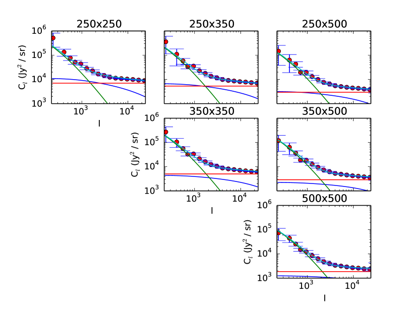
Figure 1.— Angular CIB auto- and cross-power spectra at 250, 350, 500 $\mathrm{\mu}$m from Herschel/SPIRE, together with the best-fit curves for the 1-halo (Blue line), 2-halo (Green line), shot-noise (Red line) and total power spectra (Cyan line).

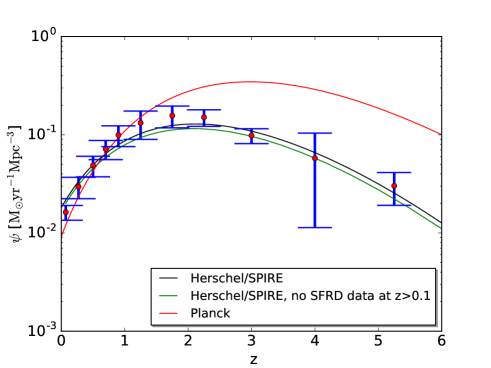
Figure 2.— Best fit estimates of the SFRD using Herschel/SPIRE CIB clustering measurements combined with a compilation of data extracted from Madau & Dickinson (2014) either in the range $\mathrm{0<z<6}$ (black line), or in $\mathrm{0<z<0.1}$ (one single measurement at $\mathrm{z=0.07}$, green line). Also plotted is the estimate from Planck Collaboration et al. (2014c) (red line).

It is important to note that there is a relevant uncertainty associated to measurements of the SFRD, especially at the high redshifts considered in this work. The compilation of measurements extrapolated from Madau & Dickinson (2014) (plotted in Fig. 2), is based on galaxy counts, and there is a number of uncertain steps in the conversion from galaxy counts and luminosities to star formation rates, mainly related to assumptions on conversion factors and dust attenuation. When considering clustering meausurements, the Planck Collaboration, using a Halo model similar to the one presented in this paper, and fitting to CIB power spectra between 217 GHz (1381 $\mu$m) and 857 GHz (350 $\mu$m) in the multipole range $\mathrm{50<l<2000}$, infer a much higher SFRD at high redshifts (Planck Collaboration et al., 2014c), respect to the values found here by fitting Herschel-SPIRE data and star formation rate density data from Madau & Dickinson (2014) (see also discussion in Cheng et al. (2016)). Similar results have been obtained by cross-correlating the CIB with the CMB lensing (Planck Collaboration et al. (2014b), see also Fig. 14 of Planck Collaboration et al. (2014c)). The reason for this discrepancy is mainly due to the different values inferred for the parameter $\mathrm{\delta}$ in Eq. 19. Planck Collaboration et al. (2014c) found $\mathrm{\delta=3.6\pm 0.2}$ (see Table 9 of Planck Collaboration et al. (2014c)), while we find $\mathrm{\delta=2.6\pm 0.2}$, compatible with (Viero et al., 2013). We checked that the fitting to star formation rate density data from Madau & Dickinson (2014) is not responsible for such a divergence, by performing an MCMC run with only one measurement of the local SFRD at $\mathrm{z=0.07}$ from Madau & Dickinson (2014) (thus being compatible with Planck’s analysis, since they use a prior on the local SFRD from Vaccari et al. (2010)). As it is clear from Fig. 2, we are not able to obtain SFRD values compatible with Planck Collaboration et al. (2014c) at high redshifts.
The disagreement between our analysis and results from Planck Collaboration et al. (2014c) can be explained by a combination of multiple factors involving our ignorance of the exact values of some key parameters, such as the amplitudes of the shot noise power spectra and the redshift evolution of the galaxy luminosity, coupled to differences in the datasets considered. CIB anisotropies are mostly sourced by galaxies at redshift $\mathrm{1<z<4}$ and, in this range, a simple power law might not be a good description of the redshift evolution of the galaxy luminosity/halo mass relation. Some semianalytic models of galaxy formation and evolution find a power law slope of $\mathrm{\sim 2.5}$ (De Lucia & Blaizot, 2007; Neistein & Dekel, 2008), but also a more gradual evolution, with different slopes for low redshift and high redshift sources (Wu et al., 2016). On the other end, observations are more in agreement with a steep evolution with redshift (Oliver et al., 2010), or with a steep evolution followed by a plateau for $\mathrm{z\sim 2}$ (Bouché et al., 2010; Weinmann et al., 2011), which is also not easily explained by theoretical arguments (Bouché et al., 2010; Weinmann et al., 2011). Planck Collaboration et al. (2014c) is indeed able to find lower values for the star formation rate density at early times, more in agreement with this work, but only when they impose the condition $\mathrm{\delta=0}$ for $\mathrm{z\geq 2}$ (see Fig. 14 of Planck Collaboration et al. (2014c)).
The differences between the two datasets in terms of angular scales and related uncertainties can also be responsible for the difference values inferred for $\mathrm{\delta}$. Planck data probe CIB anisotropies at large scales with very high precision. However, because of its angular resolution, Planck is not able to access multipoles higher than $\mathrm{l\sim 2000}$, where the 1-halo term and the shot-noise dominate the clustering, and are degenerate. Uncertainties in the contribution of these two terms to the small-scale clustering (Planck Collaboration et al. (2014c) used free amplitudes for the shot-noise power spectra, with flat priors based on current measurements, such as, e.g., Béthermin et al. (2012b)) translates in an uncertainty in the inferred constraints on the halo model parameters. On the other end, Herschel/SPIRE data probe both large and small scales, but while adding information at small scales helps disentangling the relative contributions to the total power from the 1-halo term and the shot-noise, the largest scales are measured with much larger uncertainty than Planck. Finally, Planck and Herschel probe a different frequency range, which might affects results. Thus, it is possible that the differences in the datasets used, coupled with uncertainties regarding the level of the shot-noises, and a poor description of the redshift evolution of the sources, determine different values for the parameter $\mathrm{\delta}$.
It is clear that the higher the value of the star formation rate density, the greater the value for the mean emission from all atoms and molecules. This would translate in large amplitude for the emission line power spectra. In order to be as independent as possible on the particular values of the Halo model parameters used to constrain the galaxy infrared luminosity, we compute predictions for the 3D power spectra of emission lines using both the mean values found by fitting Herschel/SPIRE data (quoted in Table 3) and the mean values quoted in Table 9 of Planck Collaboration et al. (2014c). The geometric average of these two estimates will be our best estimate of the power spectrum of the emission lines. In the rest of the paper we will focus on predictions based on these average estimates of the power spectra. In Fig. 3 we show the 3D power spectrum of [CII] emission at redshift $\mathrm{z=7}$ obtained by using mean parameter values for the Halo model parameters from Planck Collaboration et al. (2014c) (optimistic scenario), mean parameter values from our analysis of Herschel/SPIRE data, and their average. The “average” model considered here agrees at both large and small scales with the model prediction from Gong et al. (2012), which is based on a physical model that takes into account for the spontaneous, stimulated and collisional emission to compute the CII spin temperature. However, it predicts shot-noise amplitudes higher than what found in Silva et al. (2015); Lidz & Taylor (2016).

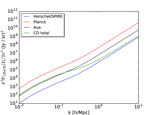
Figure 3.— Average estimate of the [CII] auto-power spectrum at redshift z=7 (black line), together with an optimistic estimate (red line) obtained from the mean values of the Halo model parameters from Planck Collaboration et al. (2014c), and an estimate (blue line) from our analysis of Herschel/SPIRE data. Also plotted is the CO power spectrum computed as the sum of the transitions from CO(3-2) to CO(7-6).

II.3. Intensity mapping power spectrum from the Halo model

The analysis presented in the previous section has been necessary to constrain the main parameters describing the galaxy SED and its dependence on halo mass and redshift.
The galaxy infrared luminosity is:

$$L_{\mathrm{IR}} = \int_{\mathrm{300\,GHz}}^{\mathrm{37.5\,THz}}\,\Theta[(1+z)\nu]d\nu$$ (22)

where the extremes of integration correspond to the wavelength range $\mathrm{8<\lambda<1000\,\mu}$m. We can use scaling relations provided in Spinoglio et al. (2012), to express the emission line luminosity $\mathrm{I_{\alpha}}$ (where $\alpha$ denotes emission lines from the atoms and molecules considered, such as carbon, oxygen, nitrogen) as a function of the constrained infrared luminosity, as:

$$log_{10}(I_{\alpha}) = (A\pm\sigma_{A})log_{10}(L_{IR})-(B\pm\sigma_{B}),$$ (23)

where all luminosities are in units of $\mathrm{10^{41}}$ erg s^-1. These scaling relations are obtained from a sample of local galaxies compiled by Brauher et al. (2008) using all observations collected by the LWS spectrometer (Clegg et al., 1996) onboard ISO (Kessler et al., 1996). Regarding the [NII] 205 $\mathrm{\mu}$m emission line, whose luminosity is not found in Spinoglio et al. (2012), we assume that it is three times weaker than the [NII] 122 $\mathrm{\mu}$m; this values is in agreement with both theoretical expectations and recent measurements (Oberst et al., 2011; Zhao et al., 2016), although it is higher than what recently found in our Galaxy (Goldsmith et al., 2015).
In Table 1 we summarize the values used for slopes, intercepts and their uncertainties, together with their associated transition, and transition temperatures from Kaufman et al. (1999); Cormier et al. (2015).
The emission line luminosity at each redshift for each halo mass can now be expressed as previosly done for the galaxy luminosity (see Eq. 15) as:

$$L_{\alpha}(M,z) = F(M,z)I_{\alpha},$$ (24)

where the term $\mathrm{F(M,z)}$ contains the global dependence on redshift and halo mass as

$$F(M,z) = L_{0}\Phi(z)\Sigma(M),$$ (25)

and we use the parameter values from Table 3 to compute the term $\mathrm{F(M,z)}$. This functional form allows us to link the emission line luminosity of a galaxy to its host halo mass, and to evolve the amplitude of all emission lines with redshifts. We note that this model assumes that the redshift evolution of all emission lines is the same, since it follows the evolution of the galaxy infrared luminosity (through the parameter $\mathrm{\delta}$). Different emission lines might have different a evolution with redshift, and more sophisticated models could incorporate redshift-dependent scaling relations for each line. However, current data do not allow us to constrain the exact dependence on redshift of each emission lines. Thus, to keep the analysis as simple as possible, we do not consider such a scenario.
It is easy to see that, assuming that each halo hosts only one galaxy (a good approximation because, at high redshift, halos are not very massive, see also Lidz et al. (2011)), and in the limit of sufficiently large scales (so that the NFW profile approaches unity), the clustering auto-power spectrum of emission line $\alpha$ can be written as:

$$P_{\alpha\alpha}(k,z) = K_{\alpha}^{2}(k,z)P_{\mathrm{lin}}(k,z),$$ (26)

where

$$K_{\alpha}(k,z) = \int_{M_{\mathrm{min}}}^{\infty}dM\frac{dN}{dM}b(M,z)\frac{L_{\mathrm{\alpha}}(M,z)}{4\pi}.$$ (27)

Introducing an effective, scale independent, bias term as:

$$b_{\mathrm{eff}}(z) = \frac{\int\,dM\frac{dN}{dM}b(M,z)\Sigma(M)}{\int\,dM\frac{dN}{dM}\Sigma(M)}$$ (28)

the clustering power spectrum of emission line $\alpha$ can be expressed as:

$$P^{\mathrm{clust}}_{\alpha\alpha}(k,z) = b_{\mathrm{eff}}^{2}(z)\bar{I}^{2}_{\alpha}(z)P_{lin}(k,z),$$ (29)

where the average specific intensity $\mathrm{\bar{I}_{\alpha}(z)}$ is:

$$\bar{I}_{\alpha}(z)=\frac{1}{4\pi}\frac{c}{H(z_{\alpha})}\frac{1}{\nu_{\alpha}}\int\,dM\frac{dN}{dM}L_{\alpha}(M,z),$$ (30)

and $z_{\alpha}$ denotes the redshift of emission of the atom or molecule $\alpha$. Analogously, the shot-noise power spectrum can be expressed as:

$$P^{\mathrm{SN}}_{\alpha\alpha} = \bar{I}_{\alpha}^{2}(z)\frac{\int\,dM\frac{dN}{dM}\Sigma(M)^{2}}{\Big{(}\int\,dM\frac{dN}{dM}\Sigma(M)\Big{)}^{2}}.$$ (31)

III. The physics of the ISM with emission lines and emission line ratios

Understanding the main heating and cooling processes of the ISM is a key goal of astronomy, because they play a fundamental role in the formation of stars, and thus in the galaxy evolution. Space missions such as Planck and Herschel, together with the Stratospheric Observatory for Infrared Astronomy (SOFIA) and the Atacama Large Millimeter Array (ALMA), are now giving new insights on these physical processes, providing spatially resolved maps of the interstellar dust in our Galaxy, and measuring atomic and molecular emission lines from the main phases of the ISM both in the Milky Way (Pineda et al., 2013, 2014; Goicoechea et al., 2015), and in external galaxies (see e.g. Stacey et al. (2010); Scoville et al. (2014); Capak et al. (2015); Gullberg et al. (2015); Blain (2015); Béthermin et al. (2016); Aravena et al. (2016)).
The gas in the ISM of galaxies is observed in three main phases; a cold and dense neutral medium (T$\mathrm{\geq 50}$K) is in rough pressure equilibrium (with $\mathrm{P/k\sim 10^{3}-10^{4}}$Kcm^-3) with a hot (T$\mathrm{\geq 10^{6}}$K), ionized phase, and an intermediate, warm (T$\mathrm{\geq\,8000}$K) phase, which can be either neutral or ionized, depending on the gas density (Wolfire et al., 1995).
Various mechanisms contribute to the heating and cooling of the ISM. For a gas with hydrogen density n, temperature T, cooling rate per unit volume of $\mathrm{\Lambda(T)}$, and heating rate per unit volume of $\mathrm{\Gamma(T)}$, the thermal balance between heating and cooling is expressed in terms of a Generalized Loss Function L:

$$L(n,T) = \Lambda(T)-\Gamma(T).$$ (32)

For a gas at constant thermal pressure nT, equilibrium occurs when $\mathrm{L=0}$ and the explicit form for $\mathrm{\Lambda}$ and $\mathrm{\Gamma}$ depends on the heating and cooling process considered, as explained below.
The investigation of the thermal balance and stability conditions of the neutral ISM started with Field et al. (1969), who first presented a model of the ISM based on two thermally stable neutral phases, cold and warm, heated by cosmic-rays. Subsequent analyses by many authors focused on the heating provided by the photoelectric ejection of electrons from dust grains by the interstellar radiation field (Draine, 1978; Wolfire et al., 1995; Kaufman et al., 1999; Wolfire et al., 2003). Most of the Far-Ultraviolet (FUV) starlight impinging on the cold neutral medium is absorbed by dust and large molecules of polycyclic aromatic hydrocarbons (PAH), and then reradiated as PAH infrared lines and infrared continuum radiation. However, as pointed out by Tielens & Hollenbach (1985b), in photodissociation regions (PDRs), the photoelectric heating of dust grains provides an efficient mechanism ($0.1\%-1\%$) at converting the FUV heating into atomic and molecular gaseous line emission. The physics of heating processes in PDRs can be understood in terms of a limited set of parameters, namely the density of Hydrogen nuclei density $\mathrm{n}$ and the incident FUV ($6$eV$\,\mathrm{<h\nu<13.6}$ eV) parametrized in units of the local interstellar field, $\mathrm{G_{0}}$ (Tielens & Hollenbach, 1985a, b; Kaufman et al., 1999), in units of the Habing field ($\mathrm{1.6\cdot 10^{-3}}$ ergs cm$\mathrm{{}^{-2}s^{-1}}$). The basic mechanism for gas heating and cooling is the following: about 10$\%$ of incident FUV photons eject photoelectrons from dust grains and PAH molecules, which cool by continuum infrared emission. The photoelectrons (with energy of about 1 eV) heat the gas by collisions, and the gas subsequently cools via FIR fine-structure line emission. The entire process thus results in the conversion of FUV photons to FIR continuum emission plus spectral line emission from various atoms and molecules. As an example, the computation of the heating due to small grains is given by (Bakes & Tielens, 1994):

$$\Gamma = 10^{-24}\epsilon\,G_{0}n_{H}\,\,\,\,\,\mathrm{erg\,cm^{-3}s^{-1}};$$ (33)

the radiation field $\mathrm{G_{0}}$ quantifies the starlight intensity, and $\epsilon$ is the fraction of FUV photons absorbed by grains which is converted to gas heating (i.e. heating efficiency), and it depends on $\mathrm{G_{0}T^{1/2}n_{e}}$, where $\mathrm{n_{e}}$ denotes the electron density Wolfire et al. (1995). A detailed calculation of the main heating processes in the ISM, including the effect from photoelectric heating, cosmic rays, soft X-rays, and photoionization of CI is presented in Wolfire et al. (1995); Meijerink & Spaans (2005).
The cooling rate $\Lambda$ of each atom/molecule depends on both the number density and the equivalent temperature of each species. A recent estimate of the cooling rate of the [CII] line for temperatures between 20 K and 400 K is (Wiesenfeld & Goldsmith, 2014):

$$\Lambda_{\mathrm{CII}} = 10^{-24}\Big{(}11.5+4.0e^{-100K/T_{\mathrm{kin}}}\Big{)}$$

$$e^{-91.25K/T_{\mathrm{kin}}}n(C^{+})n_{H_{2}}\,\,\,\,\,\mathrm{erg\,cm^{-3}s^{-1}}$$

where $\mathrm{n(C^{+})}$ denotes the carbon number density, and $\mathrm{T_{kin}}$ the kinetic temperature of the gas.
Numerical codes compute a simultaneous solution for the chemistry, radiative transfer, and thermal balance of PDRs, providing a phenomenological description of the interplay among three main parameters n, $\mathrm{G_{0}}$ and T (see e.g. Kaufman et al. (1999)) for all emission lines. The observed intensity of line emissions can thus be compared with models to constrain these parameters.
Far-infrared emission lines from forbidden atomic fine-structure transitions such as [CII] (157.7 $\mathrm{\mu}$m), [OI] (63 $\mathrm{\mu}$m and 145.5 $\mathrm{\mu}$m), are the main coolants of the neutral regions of the ISM, and provide many insights on the physics of PDRs. Other lines, such as [NII] (122 $\mathrm{\mu}$m and 205 $\mathrm{\mu}$m), [OIII] (88 $\mathrm{\mu}$m), and [NIII] (57 $\mathrm{\mu}$m), being emitted only in ionized regions, complement the study of the ISM probing a different phase.
For ground-based surveys such as Time-PILOT Crites et al. (2014) or CONCERTO, covering approximately the range $\mathrm{200<\nu<300}$ GHz, and targeting high redshift ($5<z<8$) galaxies, emission from [CII], [OI] (145 $\mathrm{\mu}$m) and [NII] (122 $\mathrm{\mu}$m and 205 $\mathrm{\mu}$m) are accessible. A future space-based survey with characteristics similar to PIXIE will be able to detect most of the main cooling lines from both PDRs and from the ionized medium of high redshift galaxies. Below we summarize some useful diagnostics of the ISM provided by these important lines (see also Cormier et al. (2015)).

• [CII] emission line: It is hard to overestimate the importance of the [CII] emission line in constraining physical properties of the interstellar medium. Because of its low ionization potential, the [CII] line arises both from ionized and neutral gas. In PDRs, the low gas critical density for collisions with Hydrogen and the low excitation temperature for the [CII] $\mathrm{{}^{2}P_{3/2}-^{2}P_{1/2}}$ transition (only 92 K, see Table 1), make $\mathrm{C^{+}}$ one of the major coolant of the neutral ISM. Moreover, since the [CII] line is generally one of the brightest lines in star-forming galaxies, it is potentially a very strong indicator of star formation rate (SFR) (Boselli et al., 2002; De Looze et al., 2011, 2014; Herrera-Camus et al., 2015). As pointed out in De Looze et al. (2011), the tight correlation between [CII] emission and mean star formation activity is due either to emission from PDRs in the immediate surroundings of star-forming regions, or emission associated to the cold ISM, thus invoking the Schmidt law to explain the link with star formation. Intensity mapping measurements of the mean amplitude of the [CII] emission line allows us to constrain the global star formation activity of the Universe at high redshift.

• [NII] (122 $\mathrm{\mu}$m and 205 $\mathrm{\mu}$m) emission lines: With a ionization potential of $\mathrm{14.53}$ eV, ionized Nitrogen is only found in the ionized phase of the ISM. The two infrared [NII] lines are due to the splitting of the ground state of N⁺ into three fine-structure levels, which are excited mainly by collisions with free electrons in HII regions, with critical densities of 290 cm^-3 and 44 ^-3 for [NII] (122 $\mathrm{\mu}$m) and [NII] (205 $\mathrm{\mu}$m) respectively, assuming $\mathrm{T_{e}=8000}$ K, see Herrera-Camus et al. (2016); Hudson & Bell (2004). Being in the same ionization stage, their ratio directly determines the electron density of the ionized gas in HII regions. For electron densities $n_{e}$ larger than $10$ cm^-3, the 122/205 $\mathrm{\mu}$m line ratio R_122/205 increases as a function of $n_{e}$, starting from R${}_{\mathrm{122/205}}\sim 0.6$ for $\mathrm{n_{e}\sim 10}$ cm^-3, and reaching the value R${}_{\mathrm{122/205}}\mathrm{\sim 3}$ (the value used in this paper) for $\mathrm{n_{e}\sim\,100}$ cm^-3 (Tayal, 2011; Goldsmith et al., 2015).
  Moreover, combined measurements of line emission from [NII] and [CII] can be used to estimate the amount of [CII] emission coming from the ionized medium (Malhotra et al., 2001; Oberst et al., 2006; Decarli et al., 2014; Hughes et al., 2016). Recently Goldsmith et al. (2015), using data from the PACS and HIFI instruments onboard Herschel, estimated that between 1/3 and 1/2 of the [CII] emission from sources in the Galactic plane arise from the ionized gas. The [NII]/[CII] ratio is also useful to estimate the metallicity of a galaxy (Nagao et al., 2012). Finally, the [NII] emission lines, arising from gas ionized by O and B type stars, directly constrains the ionizing photon rate, and thus the star formation rate (Bennett et al., 1994; McKee & Williams, 1997).

• Oxygen 63 $\mathrm{\mu}$m and 145 $\mathrm{\mu}$m lines: Oxygen has a ionization potential of $\mathrm{13.62}$ eV, just above that of hydrogen. The $\mathrm{[OI]}$ (63 $\mathrm{\mu}$m) and $\mathrm{[OI]}$ (145 $\mathrm{\mu}$m) line emissions come from PDRs and, together with [CII], are a major coolant of the ISM. However, because their fine structure transitions are excited at high temperatures (228 K and 326 K respectively, against 91 K of [CII]), and their critical densities are quite high ($\mathrm{\sim\,5e5\,cm^{-3}}$ and $\mathrm{\sim\,1e5\,cm^{-3}}$ for [OI] 63 $\mathrm{\mu}$m and [OI] 145 $\mathrm{\mu}$m respectively) they contribute significantly to the cooling of the ISM only for high FUV fields and/or high densities. The measurement of the mean amplitude of the [OI] lines with intensity mapping would give us clues regarding the mean value of the $\mathrm{G_{0}}$ field and the mean density of PDRs at high redshifts (Meijerink et al., 2007).

The intensity mapping technique would constrain the mean amplitude of multiple emission lines, together with their ratio, thus probing mean properties (such as mean radiation field, mean electron density in HII regions, mean density of various atoms, molecules) at high redshifts.

IV. Multiple cross-correlations constrain the physics of the ISM

As previously stated, the cross-correlation signal between different emission lines coming from the same redshift is important not only to avoid contamination from foreground lines (assuming that, at the frequencies considered in the cross-correlation measurements, foregrounds are not correlated), but also to help constraining the mean amplitude of each signal. This is particularly true at sufficiently small scales, where the SNR is larger. If we assume that all lines are emitted by the same objects (a reasonable assumption, especially if the emission lines are not distant from each other, as in the case of the FIR lines such as [CII], [NII] and [OI]), it will be possible to constrain the mean amplitudes of emission lines $\mathrm{I}_{i=1,...N}$, just by looking at all cross-correlation power spectra.
For a survey working in a given frequency range where N lines are detected, there are $\mathrm{N(N-1)/2}$ cross-correlation measurements to be performed and, assuming there is perfect correlation among lines, it is sufficient that $\mathrm{N\geq 3}$ to be able to constrain the mean emission from all lines.
The chances of detecting auto- and cross-power spectra strongly depend on the amplitude of the spectra, which, as already seen, is very uncertain. In the following we will consider predicted measurements of multiple combinations of emission line power spectra for two different surveys. The first one corresponds to a survey of the [CII] emission line similar to the proposed CONCERTO. The second one, referred in literature as CII-Stage II, and described in Silva et al. (2015); Lidz & Taylor (2016), is more sensitive, and corresponds to an evolution of currently planned [CII] surveys.
As already emphasized, emission line power spectra are strongly contaminated by interlopers lines emitted by molecules at different redshifts. In case of [CII], the main confusion results from foreground emission of CO molecules undergoing rotational transitions between states J and J-1. As an example, [CII] emission from $\mathrm{z=6}$ is observed at frequency $\mathrm{\nu_{obs}=271.6}$ GHz, and it is mainly contaminated by CO rotational transitions $\mathrm{J=3\rightarrow 2}$ ($\mathrm{z=0.27}$), $\mathrm{J=4\rightarrow 3}$ ($\mathrm{z=0.70}$), $\mathrm{J=5\rightarrow 4}$ ($\mathrm{z=1.12}$), $\mathrm{J=6\rightarrow 5}$ ($\mathrm{z=1.54}$), and $\mathrm{J=7\rightarrow 6}$ ($\mathrm{z=1.97}$). Emission lines beyond this transition have a negligible contribution to the total foreground due to CO molecules, and we will not consider them in the rest of the paper.
Using linear scaling relations from Visbal & Loeb (2010) to express the amplitude of the various CO emission lines as a function of the infrared luminosity, it is possible to estimate the contamination due to the main CO rotational lines. In the following, when plotting the [CII] auto-power spectra at various redshits, we will also plot the CO auto-power spectrum computed as the sum of the the main CO rotational transitions involved (from $\mathrm{3\rightarrow 2}$ to $\mathrm{7\rightarrow 6}$), in order to highlight the amplitude of this foreground.

V. Experimental setups and predictions

In order to measure high-redshift fluctuations with sufficient SNR at the scales of interest, it is important to optimize the survey area. All predictions considered in this section are based on measurements spanning a redshift range $\mathrm{\Delta\,z\sim 0.6}$ which corresponds to a frequency range of $\mathrm{B_{\nu}}\sim 20$ GHz at $z=7$ for the [CII] line. We follow Gong et al. (2012) to compute uncertainties on the power spectra.

$\begin{array}[]{ccc}\includegraphics[width=184.9429pt]{./fig_concerto_spectraCIIxCII_z50.pdf}\includegraphics[width=184.9429pt]{./fig_concerto_spectraCIIxNII2_z50.pdf}\includegraphics[width=184.9429pt]{./fig_concerto_spectraCIIxOI1_z50.pdf}\end{array}$

Figure 4.— Predicted [CII] auto-power spectrum and cross-power spectra between [CII] and [NII] (205.2 $\mathrm{\mu}$m), and [OI](145.5 $\mathrm{\mu}$m), at $\mathrm{z=5}$ computed for the survey CONCERTO. Also plotted in the left panel (green line) is the total CO power spectrum computed as the sum of the contributions from CO(3-2) to CO(7-6).

$\begin{array}[]{cc}\includegraphics[width=241.84842pt]{./fig_concerto_spectraCIIxCII_z60.pdf}\includegraphics[width=241.84842pt]{./fig_concerto_spectraCIIxNII1_z60.pdf}\\ \includegraphics[width=241.84842pt]{./fig_concerto_spectraCIIxNII2_z60.pdf}\includegraphics[width=241.84842pt]{./fig_concerto_spectraCIIxOI1_z60.pdf}\end{array}$

Figure 5.— Predicted [CII] and total CO (3-2 to 7-6) auto-power spectra (left panel, black and green line respectively) at redshift $\mathrm{z=6.0}$, and cross-spectra [CII]x[NII] (121.9 $\mathrm{\mu}$m), [CII]x[NII](205.2 $\mathrm{\mu}$m), and [CII]x[OI](145.5 $\mathrm{\mu}$m) at z=6 for the survey CONCERTO.

$\begin{array}[]{ccc}\includegraphics[width=184.9429pt]{./fig_stage2_spectraCIIxCII_z60.pdf}\includegraphics[width=184.9429pt]{./fig_stage2_spectraCIIxNII2_z60.pdf}\includegraphics[width=184.9429pt]{./fig_stage2_spectraCIIxOI1_z60.pdf}\end{array}$

Figure 6.— Predictions for both [CII] and total CO (3-2 to 7-6) auto-power spectra (left panel, black and green line respectively), and cross-spectra [CII]x[NII](205.2 $\mathrm{\mu}$m), and [CII]x[OI](145.5 $\mathrm{\mu}$m) at z=6 for a CII-stage II survey. All spectra are detected with high SNR.

Instrument parameters	CONCERTO	CII-Stage II
Dish size (m)	12	10
Survey Area (deg2)	2	100
Frequency range (GHz)	200-360	200-300
Frequency resolution (GHz)	1.5	0.4
Number of spectrometers	1500	64
On-sky integration time (hr)	1500	2000
NEFD on sky (mJy$\sqrt{(}sec)$	155	5

Table 3 Instrumental parameters for the two surveys, CONCERTO and CII-Stage II, considered.

The primary goal of the first survey considered, called CONCERTO, is to detect [CII] fluctuations in the redshift range $\mathrm{4.5<z<8.5}$. It is based on a spectrometer working in the frequency range $\mathrm{200<\nu<360}$ GHz, with spectral resolution $\mathrm{\delta_{\nu}\sim 1.5}$ GHz. Such a frequency window imposes the use of a so-called “sub-millimetre” telescope, with primary aperture size $\mathrm{D=12}$ m, and moderate angular resolution. The instrumental noise is thus computed for a total observing time of $\mathrm{t_{survey}=1500}$ hours, and a number of spectrometers $\mathrm{N_{sp}}=1500$. The survey area considered here is two square degrees, and is optimized to ensure high SNR in the wavenumber range of $\mathrm{0.1<k<1}$ h / Mpc.
Accounting for realistic observational conditions and the total atmospheric transmission, the Noise Equivalent Flux density (NEFD), computed as the sensitivity per single pixel divided by the square root of the number of spectrometers, is equal to $\mathrm{NEFD=155}$ mJy sec^1/2, for a spectral resolution of $\mathrm{\delta_{\nu}=1.5}$ GHz. The on-sky sensitivity $\mathrm{\sigma_{N}}$ can be expressed as:

$$\sigma_{\mathrm{N}}=\frac{\mathrm{NEFD}}{\Delta\Omega_{\mathrm{beam}}}$$ (35)

where

$$\Delta\Omega_{\mathrm{beam}} = 2\pi\Big{(}\frac{\theta_{\mathrm{beam}}}{2.355}\Big{)}^{2}$$ (36)

is the beam area (in steradians), and the beam FWHM is given by:

$$\theta_{\mathrm{beam}} = 1.22\lambda_{\mathrm{obs}}/D$$ (37)

where $\mathrm{\lambda_{\mathrm{obs}}}$ is the observed wavelength. Values for $\mathrm{\sigma_{N}}$ at $\mathrm{z=5}$, $\mathrm{z=6}$, and $\mathrm{z=7}$ are 15, 11, and 8.3 MJy/sr$\mathrm{\sqrt{(}sec)}$ respectively.
The observing time per pixel is given by:

$$t_{\mathrm{obs}} = t_{\mathrm{survey}}N_{\mathrm{sp}}\frac{\Delta\Omega_{\mathrm{pix}}}{\Delta\Omega_{\mathrm{survey}}},$$ (38)

where $\mathrm{\Delta\Omega_{survey}}$ is the total survey area covered.
Assuming a spherically averaged power spectrum measurement, and a directionally independent on sky sensitivity $\sigma_{\mathrm{N}}$, the variance of the power spectrum is:

$$\mathrm{var}[\bar{P}_{\alpha}(k)]=\frac{[P_{\alpha}(k)+\bar{P}_{\alpha}^{\mathrm{N}}(k)]^{2}}{N_{\mathrm{m}}(k,z)},$$ (39)

where $\mathrm{N_{m}(k,z)}$ denotes the number of modes at each wavenumber:

$$N_{m}(k,z)=2\pi\,k^{2}\Delta\,k\frac{V_{s}}{(2\pi)^{3}};$$ (40)

the term $\mathrm{\Delta\,k}$ is the Fourier bin size, and V_s(z) is the survey volume, expressed as:

$$V_{s}(z)=\chi(z)^{2}\bar{y}\Delta\Omega_{\mathrm{survey}}B_{\nu}.$$ (41)

The averaged noise power spectrum in Eq. 39 is:

$$\bar{P}_{\alpha}^{\mathrm{N}}(k)=V_{\mathrm{pix}}\frac{\sigma_{N}^{2}}{t_{\mathrm{obs}}};$$ (42)

where the volume surveyed by each pixel is:

$$V_{\mathrm{pix}} = \chi(z)^{2}\bar{y}_{\alpha}(z)\Omega_{\mathrm{beam}}\delta_{\nu},$$ (43)

with

$$\bar{y}_{\alpha}(z) = \lambda_{\alpha}(1+z)^{2}/H(z),$$ (44)

and $\mathrm{\lambda_{\alpha}}$ is the wavelength of the line $\alpha$ is the rest frame.
In Fig. 4 we plot measurements of the [CII] auto-power spectrum, together with [CII]x[OI] (145.5 $\mathrm{\mu}$m), and [CII]x[NII] (205.2 $\mathrm{\mu}$m) cross-power spectra at $\mathrm{z=5.0}$ for CONCERTO. For wavenumbers in the range $\mathrm{0.1<k<1}$ h / Mpc, the [CII] auto-power spectrum will be detected with high significance ($\mathrm{SNR>50}$), while the [CII] cross-correlations with oxygen and nitrogen at these scales will not be very significant (SNR$\mathrm{\sim 3}$ and SNR$\mathrm{\sim 0.5}$ respectively). However, considering smaller scales (larger wavenumbers) the SNR increases significantly, and it will enable us to constrain the mean quantities $\mathrm{I_{[CII]}}$, $\mathrm{I_{[OI]}}$, and $\mathrm{I_{[NII]}}$. Given the CONCERTO frequency coverage, at $\mathrm{z=6.0}$ it is possible to add the cross-correlation with [NII] (122 $\mathrm{\mu}$m). As shown in Fig. 5, the cross-correlation of carbon with oxygen and nitrogen seems to be barely detectable at linear scales. However, in the non-linear regime, it might still be possible to measure these cross-correlations, and thus constrain the mean amplitude of these emission lines. As already described in Sect. III, by looking at the cross-power spectra [CII]x[NII] (121.9 $\mathrm{\mu)}$m, and [CII]x[NII] (205.2 $\mathrm{\mu}$m), we would be able to measure the mean ratio [NII] (205.2 $\mathrm{\mu}$m) / [NII] (121.9 $\mathrm{\mu}$m), which is useful not only to constrain the electron density of the low-ionized gas in HII regions, but also to infer the mean emission of [CII] from PDRs, and to constrain the global star formation rate. The mean ratio between [OI] (145.5 $\mathrm{\mu}$m) and CII is also a useful diagnostic of mean properties of properties of PDRs, such as the hydrogen density and the strength of the radiation field.
The second experimental setup, called CII-Stage II, has been introduced in Silva et al. (2015) as an appropriate baseline to ensure detection of [CII] spectra in case of a pessimistic [CII] amplitude (see also Lidz & Taylor (2016)). It consists of a dish with diameter $\mathrm{D=10}$ m, with $\mathrm{16000}$ bolometers and $N_{\mathrm{sp}}=64$ beam spectrometers, observing in the frequency range $\mathrm{200<\nu<300}$ GHz, with a frequency resolution of 0.4 GHz. The total survey area is 100 deg² for a total observing time of t${}_{\mathrm{survey}}=2000$ hours, and a NEFD of 5 mJy sec^1/2.
As it appears from Fig. 6, the cross-correlation of carbon with oxygen and nitrogen is now detectable with high SNR at $\mathrm{z=6}$. A space-based survey, being not limited by the atmosphere, would be able to perform measurements on a still wider frequency range, and thus perform measurements of high-redshift correlations with other interesting lines such as [OI] (63 $\mathrm{\mu}$m), [OIII] (88 $\mathrm{\mu}$m), [NIII] 57 $\mathrm{\mu}$m, and [CI] (370 $\mathrm{\mu}$m and 609 $\mathrm{\mu}$m.

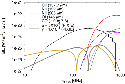
Figure 7.— Amplitudes of main emission lines that can be observed in the frequency range $\mathrm{\nu_{obs}=[10-1000]}$ GHz, together with the expected spectral distortions $\mu$ and $y$.

VI. Discussion

We have developed a consistent framework to compute predictions of 3D power spectra of multiple FIR cooling lines of the ISM. Using measurements of CIB power spectra, together with measurements of star formation rate density from Madau & Dickinson (2014), it is possible to constrain the galaxy FIR luminosity at all redshift, which can be directly linked to emission line amplitudes through scaling relation from Spinoglio et al. (2012). Present and upcoming ground-based surveys aiming at measuring the power spectrum of the bright [CII] line, should be able to detect also the cross-correlation between the [CII] line and other lines produced in all phases of the ISM, such as [NII] (122 $\mathrm{\mu}$m and 205 $\mathrm{\mu}$m), and [OI] (145.5 $\mathrm{\mu}$m). Multiple measurements of cross-power spectra between [CII] and other emission lines will allow us to constrain the mean amplitude of each signal, and they will be key to gain insight into the mean properties of the ISM. Future surveys, such as PIXIE (Kogut et al., 2011, 2014), working in a broad frequency range, will detect many more atomic and molecular lines emitted from moderate to high redshift with high SNR, allowing us to obtain multiple probes of all phases of the ISM. Moreover, the cross-correlation of the target line with galaxy number densities from future surveys such as, e.g., LSST (LSST Science Collaboration et al., 2009), will be a powerful method to eliminate line foregrounds.
Line emissions from multiple atoms/molecules at multiple redshifts are also an important foreground for future surveys aiming at constraining CMB spectral distortions. In Fig. 7 we plot $\mathrm{\mu}$-type and y-type spectral distortions with $\mathrm{\mu=5\cdot 10^{-8}}$ and $\mathrm{y=1\cdot 10^{-8}}$, corresponding to the current PIXIE $\mathrm{5\sigma}$ sensitivity limits, together with the sum of the spectra from carbon monoxide emission lines (from $\mathrm{J=1\rightarrow 0}$ to $\mathrm{J=7\rightarrow 6}$), and the spectra from all emission lines considered in this work. The CO spectra have been computed using scaling relations from Visbal & Loeb (2010) to link the CO line emission to the star formation rate, and the Kennicutt relation to express the star formation rate in terms of the galaxy infrared luminosity (Kennicutt, 1998). The amplitude of the global signal from CO lines is similar to what found by Mashian et al. (2016) using a radiative transfer modeling technique, even if the shape is slightly different.
We note that, even if foreground lines do not have a simple spectral dependence, unlike other foregrounds that can be modeled with power law such as synchrotron or thermal dust, their shape is still monotonic in frequency, and thus very different with respect to the CMB spectral distortions. However, foreground subtraction will require a very good knowledge of the amplitude and shape of the total signal provided by the sum of these lines. The intensity mapping technique, by constraining the mean amplitude of the signal in multiple redshift bins, will help constraining the global contamination signal.
Finally, it is clear that an aggressive program to model the amplitude of all emission lines at all redshifts is necessary to have a detailed interpretation of upcoming measurements. Scaling relations are useful to work with, but they provide little information on the main physical mechanisms governing the line emission. Moreover, they are based on few observations performed at some given redshift, and their redshift evolution is not very well known. Different physical conditions can dominate the line emission at different epochs, strongly affecting the amplitude of the signal. As an example, at high redshift, the CMB strongly suppresses the [CII] emission from the cold neutral medium, leaving only the emission from PDRs (Vallini et al., 2015). The redshift evolution of the galaxy infrared luminosity (which governs the evolution of the line emission in our model) is determined by the power law parameter $\delta$ (see Eq. 19), which, as stated earlier, is quite uncertain, especially at high redshifts. On the other hand, semi-analytic models of galaxy formation and evolution often involve a large number of assumptions and free parameters, and such a complexity makes them difficult to use. A third approach, intermediate between the two, and based on present and upcoming measurements from, e.g. ALMA and SOFIA, should be developed to model the line intensity of all relevant emission lines, together with their redshift evolution. Such a model, possibly based on the physics of photodissociation regions, ionized medium, and molecular clouds, will offer an important guidance in interpreting upcoming and future intensity mapping observations, and thus constrain the mean properties of high-redshift galaxies.

References

- Aravena et al. (2016) Aravena, M., Decarli, R., Walter, F., et al. 2016, ArXiv e-prints, arXiv:1607.06772
- Bakes & Tielens (1994) Bakes, E. L. O., & Tielens, A. G. G. M. 1994, ApJ, 427, 822
- Battye et al. (2004) Battye, R. A., Davies, R. D., & Weller, J. 2004, MNRAS, 355, 1339
- Behroozi et al. (2013) Behroozi, P. S., Wechsler, R. H., & Conroy, C. 2013, ApJ, 770, 57
- Bennett et al. (1994) Bennett, C. L., Fixsen, D. J., Hinshaw, G., et al. 1994, ApJ, 434, 587
- Benson et al. (2003) Benson, A. J., Bower, R. G., Frenk, C. S., et al. 2003, ApJ, 599, 38
- Bernard-Salas et al. (2012) Bernard-Salas, J., Habart, E., Arab, H., et al. 2012, A&A, 538, A37
- Bertone et al. (2005) Bertone, S., Stoehr, F., & White, S. D. M. 2005, MNRAS, 359, 1201
- Béthermin et al. (2012a) Béthermin, M., Doré, O., & Lagache, G. 2012a, A&A, 537, L5
- Béthermin et al. (2012b) Béthermin, M., Daddi, E., Magdis, G., et al. 2012b, ApJ, 757, L23
- Béthermin et al. (2016) Béthermin, M., De Breuck, C., Gullberg, B., et al. 2016, A&A, 586, L7
- Blain (2015) Blain, A. W. 2015, in Astronomical Society of the Pacific Conference Series, Vol. 499, Revolution in Astronomy with ALMA: The Third Year, ed. D. Iono, K. Tatematsu, A. Wootten, & L. Testi
- Blain et al. (2003) Blain, A. W., Barnard, V. E., & Chapman, S. C. 2003, MNRAS, 338, 733
- Boselli et al. (2002) Boselli, A., Gavazzi, G., Lequeux, J., & Pierini, D. 2002, A&A, 385, 454
- Bouché et al. (2010) Bouché, N., Dekel, A., Genzel, R., et al. 2010, ApJ, 718, 1001
- Bradford et al. (2015) Bradford, C. M., Goldsmith, P. F., Bolatto, A., et al. 2015, ArXiv e-prints, arXiv:1505.05551
- Brauher et al. (2008) Brauher, J. R., Dale, D. A., & Helou, G. 2008, ApJS, 178, 280
- Breysse et al. (2014) Breysse, P. C., Kovetz, E. D., & Kamionkowski, M. 2014, MNRAS, 443, 3506
- Breysse et al. (2015) —. 2015, MNRAS, 452, 3408
- Bull et al. (2015) Bull, P., Ferreira, P. G., Patel, P., & Santos, M. G. 2015, ApJ, 803, 21
- Capak et al. (2015) Capak, P. L., Carilli, C., Jones, G., et al. 2015, Nature, 522, 455
- Carilli (2011) Carilli, C. L. 2011, ApJ, 730, L30
- Carilli et al. (2016) Carilli, C. L., Chluba, J., Decarli, R., et al. 2016, ArXiv e-prints, arXiv:1607.06773
- Chang et al. (2010) Chang, T.-C., Pen, U.-L., Bandura, K., & Peterson, J. B. 2010, Nature, 466, 463
- Cheng et al. (2016) Cheng, Y.-T., Chang, T.-C., Bock, J., Bradford, C. M., & Cooray, A. 2016, ArXiv e-prints, arXiv:1604.07833
- Clegg et al. (1996) Clegg, P. E., Ade, P. A. R., Armand, C., et al. 1996, A&A, 315, L38
- Cooray & Sheth (2002) Cooray, A., & Sheth, R. 2002, Phys. Rep., 372, 1
- Cormier et al. (2015) Cormier, D., Madden, S. C., Lebouteiller, V., et al. 2015, A&A, 578, A53
- Crites et al. (2014) Crites, A. T., Bock, J. J., Bradford, C. M., et al. 2014, in Proc. SPIE, Vol. 9153, Millimeter, Submillimeter, and Far-Infrared Detectors and Instrumentation for Astronomy VII, 91531W
- Croton et al. (2006) Croton, D. J., Springel, V., White, S. D. M., et al. 2006, MNRAS, 365, 11
- De Breuck et al. (2011) De Breuck, C., Maiolino, R., Caselli, P., et al. 2011, A&A, 530, L8
- De Looze et al. (2011) De Looze, I., Baes, M., Fritz, J., Bendo, G. J., & Cortese, L. 2011, Baltic Astronomy, 20, 463
- De Looze et al. (2014) De Looze, I., Cormier, D., Lebouteiller, V., et al. 2014, A&A, 568, A62
- De Lucia & Blaizot (2007) De Lucia, G., & Blaizot, J. 2007, MNRAS, 375, 2
- De Zotti et al. (2016) De Zotti, G., Negrello, M., Castex, G., Lapi, A., & Bonato, M. 2016, J. Cosmology Astropart. Phys, 3, 047
- Decarli et al. (2014) Decarli, R., Walter, F., Carilli, C., et al. 2014, ApJ, 782, L17
- Dekel & Birnboim (2006) Dekel, A., & Birnboim, Y. 2006, MNRAS, 368, 2
- Doré et al. (2014) Doré, O., Bock, J., Ashby, M., et al. 2014, ArXiv e-prints, arXiv:1412.4872
- Doré et al. (2016) Doré, O., Werner, M. W., Ashby, M., et al. 2016, ArXiv e-prints, arXiv:1606.07039
- Draine (1978) Draine, B. T. 1978, ApJS, 36, 595
- Draine (2011) —. 2011, Physics of the Interstellar and Intergalactic Medium
- Duffy et al. (2010) Duffy, A. R., Schaye, J., Kay, S. T., et al. 2010, MNRAS, 405, 2161
- Field et al. (1969) Field, G. B., Goldsmith, D. W., & Habing, H. J. 1969, ApJ, 155, L149
- Fonseca et al. (2016) Fonseca, J., Silva, M., Santos, M. G., & Cooray, A. 2016, ArXiv e-prints, arXiv:1607.05288
- Furlanetto et al. (2006) Furlanetto, S. R., Oh, S. P., & Briggs, F. H. 2006, Phys. Rep., 433, 181
- Goicoechea et al. (2015) Goicoechea, J. R., Teyssier, D., Etxaluze, M., et al. 2015, ApJ, 812, 75
- Goldsmith et al. (2015) Goldsmith, P. F., Yıldız, U. A., Langer, W. D., & Pineda, J. L. 2015, ApJ, 814, 133
- Gong et al. (2012) Gong, Y., Cooray, A., Silva, M., et al. 2012, ApJ, 745, 49
- Gong et al. (2011) Gong, Y., Cooray, A., Silva, M. B., Santos, M. G., & Lubin, P. 2011, ApJ, 728, L46
- Gullberg et al. (2015) Gullberg, B., De Breuck, C., Vieira, J. D., et al. 2015, MNRAS, 449, 2883
- Hall et al. (2010) Hall, N. R., Keisler, R., Knox, L., et al. 2010, ApJ, 718, 632
- Herrera-Camus et al. (2015) Herrera-Camus, R., Bolatto, A. D., Wolfire, M. G., et al. 2015, ApJ, 800, 1
- Herrera-Camus et al. (2016) Herrera-Camus, R., Bolatto, A., Smith, J. D., et al. 2016, ArXiv e-prints, arXiv:1605.03180
- Hollenbach & Tielens (1999) Hollenbach, D. J., & Tielens, A. G. G. M. 1999, Reviews of Modern Physics, 71, 173
- Hudson & Bell (2004) Hudson, C. E., & Bell, K. L. 2004, VizieR Online Data Catalog, 343
- Hughes et al. (2016) Hughes, T. M., Baes, M., Schirm, M. R. P., et al. 2016, A&A, 587, A45
- Iono et al. (2006) Iono, D., Yun, M. S., Elvis, M., et al. 2006, ApJ, 645, L97
- Ivison et al. (2010) Ivison, R. J., Swinbank, A. M., Swinyard, B., et al. 2010, A&A, 518, L35
- Kaufman et al. (1999) Kaufman, M. J., Wolfire, M. G., Hollenbach, D. J., & Luhman, M. L. 1999, ApJ, 527, 795
- Keating et al. (2016) Keating, G. K., Marrone, D. P., Bower, G. C., et al. 2016, ArXiv e-prints, arXiv:1605.03971
- Keating et al. (2015) Keating, G. K., Bower, G. C., Marrone, D. P., et al. 2015, ApJ, 814, 140
- Kennicutt (1998) Kennicutt, Jr., R. C. 1998, ARA&A, 36, 189
- Kessler et al. (1996) Kessler, M. F., Steinz, J. A., Anderegg, M. E., et al. 1996, A&A, 315, L27
- Kogut et al. (2011) Kogut, A., Fixsen, D. J., Chuss, D. T., et al. 2011, J. Cosmology Astropart. Phys, 7, 025
- Kogut et al. (2014) Kogut, A., Chuss, D. T., Dotson, J., et al. 2014, in Proc. SPIE, Vol. 9143, Space Telescopes and Instrumentation 2014: Optical, Infrared, and Millimeter Wave, 91431E
- Lewis & Bridle (2002) Lewis, A., & Bridle, S. 2002, Phys. Rev. D, 66, 103511
- Li et al. (2016) Li, T. Y., Wechsler, R. H., Devaraj, K., & Church, S. E. 2016, ApJ, 817, 169
- Lidz et al. (2011) Lidz, A., Furlanetto, S. R., Oh, S. P., et al. 2011, ApJ, 741, 70
- Lidz & Taylor (2016) Lidz, A., & Taylor, J. 2016, ArXiv e-prints, arXiv:1604.05737
- Limber (1954) Limber, D. N. 1954, ApJ, 119, 655
- LSST Science Collaboration et al. (2009) LSST Science Collaboration, Abell, P. A., Allison, J., et al. 2009, ArXiv e-prints, arXiv:0912.0201
- Madau & Dickinson (2014) Madau, P., & Dickinson, M. 2014, ARA&A, 52, 415
- Madau et al. (1997) Madau, P., Meiksin, A., & Rees, M. J. 1997, ApJ, 475, 429
- Maiolino et al. (2009) Maiolino, R., Caselli, P., Nagao, T., et al. 2009, A&A, 500, L1
- Maiolino et al. (2005) Maiolino, R., Cox, P., Caselli, P., et al. 2005, A&A, 440, L51
- Malhotra et al. (2001) Malhotra, S., Kaufman, M. J., Hollenbach, D., et al. 2001, ApJ, 561, 766
- Mashian et al. (2016) Mashian, N., Loeb, A., & Sternberg, A. 2016, MNRAS, 458, L99
- McKee & Williams (1997) McKee, C. F., & Williams, J. P. 1997, ApJ, 476, 144
- Meijerink & Spaans (2005) Meijerink, R., & Spaans, M. 2005, A&A, 436, 397
- Meijerink et al. (2007) Meijerink, R., Spaans, M., & Israel, F. P. 2007, A&A, 461, 793
- Nagao et al. (2012) Nagao, T., Maiolino, R., De Breuck, C., et al. 2012, A&A, 542, L34
- Navarro et al. (1997) Navarro, J. F., Frenk, C. S., & White, S. D. M. 1997, ApJ, 490, 493
- Neistein & Dekel (2008) Neistein, E., & Dekel, A. 2008, MNRAS, 383, 615
- Oberst et al. (2011) Oberst, T. E., Parshley, S. C., Nikola, T., et al. 2011, ApJ, 739, 100
- Oberst et al. (2006) Oberst, T. E., Parshley, S. C., Stacey, G. J., et al. 2006, ApJ, 652, L125
- Oliver et al. (2010) Oliver, S., Frost, M., Farrah, D., et al. 2010, MNRAS, 405, 2279
- Pineda et al. (2014) Pineda, J. L., Langer, W. D., & Goldsmith, P. F. 2014, A&A, 570, A121
- Pineda et al. (2013) Pineda, J. L., Langer, W. D., Velusamy, T., & Goldsmith, P. F. 2013, A&A, 554, A103
- Planck Collaboration (2014) Planck Collaboration. 2014, A&A, 566, A55
- Planck Collaboration et al. (2014a) Planck Collaboration, Ade, P. A. R., Aghanim, N., et al. 2014a, A&A, 571, A16
- Planck Collaboration et al. (2014b) —. 2014b, A&A, 571, A18
- Planck Collaboration et al. (2014c) —. 2014c, A&A, 571, A30
- Pullen et al. (2013) Pullen, A. R., Chang, T.-C., Doré, O., & Lidz, A. 2013, ApJ, 768, 15
- Pullen et al. (2014) Pullen, A. R., Doré, O., & Bock, J. 2014, ApJ, 786, 111
- Righi et al. (2008) Righi, M., Hernández-Monteagudo, C., & Sunyaev, R. A. 2008, A&A, 489, 489
- Scoville et al. (2014) Scoville, N., Aussel, H., Sheth, K., et al. 2014, ApJ, 783, 84
- Shang et al. (2012) Shang, C., Haiman, Z., Knox, L., & Oh, S. P. 2012, MNRAS, 421, 2832
- Shaver et al. (1999) Shaver, P. A., Windhorst, R. A., Madau, P., & de Bruyn, A. G. 1999, A&A, 345, 380
- Silk (2003) Silk, J. 2003, MNRAS, 343, 249
- Silva et al. (2015) Silva, M., Santos, M. G., Cooray, A., & Gong, Y. 2015, ApJ, 806, 209
- Spinoglio et al. (2012) Spinoglio, L., Dasyra, K. M., Franceschini, A., et al. 2012, ApJ, 745, 171
- Stacey et al. (1991) Stacey, G. J., Geis, N., Genzel, R., et al. 1991, ApJ, 373, 423
- Stacey et al. (2010) Stacey, G. J., Hailey-Dunsheath, S., Ferkinhoff, C., et al. 2010, ApJ, 724, 957
- Suginohara et al. (1999) Suginohara, M., Suginohara, T., & Spergel, D. N. 1999, ApJ, 512, 547
- Tayal (2011) Tayal, S. S. 2011, ApJS, 195, 12
- Tielens & Hollenbach (1985a) Tielens, A. G. G. M., & Hollenbach, D. 1985a, ApJ, 291, 747
- Tielens & Hollenbach (1985b) —. 1985b, ApJ, 291, 722
- Tinker et al. (2008) Tinker, J., Kravtsov, A. V., Klypin, A., et al. 2008, ApJ, 688, 709
- Tinker et al. (2010) Tinker, J. L., Robertson, B. E., Kravtsov, A. V., et al. 2010, ApJ, 724, 878
- Uzgil et al. (2014) Uzgil, B. D., Aguirre, J. E., Bradford, C. M., & Lidz, A. 2014, ApJ, 793, 116
- Vaccari et al. (2010) Vaccari, M., Marchetti, L., Franceschini, A., et al. 2010, A&A, 518, L20
- Vallini et al. (2015) Vallini, L., Gallerani, S., Ferrara, A., Pallottini, A., & Yue, B. 2015, ApJ, 813, 36
- Viero et al. (2013) Viero, M. P., Wang, L., Zemcov, M., et al. 2013, ApJ, 772, 77
- Visbal et al. (2015) Visbal, E., Haiman, Z., & Bryan, G. L. 2015, MNRAS, 450, 2506
- Visbal & Loeb (2010) Visbal, E., & Loeb, A. 2010, J. Cosmology Astropart. Phys, 11, 016
- Visbal et al. (2011) Visbal, E., Trac, H., & Loeb, A. 2011, J. Cosmology Astropart. Phys, 8, 010
- Wagg et al. (2010) Wagg, J., Carilli, C. L., Wilner, D. J., et al. 2010, A&A, 519, L1
- Weinmann et al. (2011) Weinmann, S. M., Neistein, E., & Dekel, A. 2011, MNRAS, 417, 2737
- Wiesenfeld & Goldsmith (2014) Wiesenfeld, L., & Goldsmith, P. F. 2014, ApJ, 780, 183
- Wolfire et al. (1995) Wolfire, M. G., Hollenbach, D., McKee, C. F., Tielens, A. G. G. M., & Bakes, E. L. O. 1995, ApJ, 443, 152
- Wolfire et al. (2003) Wolfire, M. G., McKee, C. F., Hollenbach, D., & Tielens, A. G. G. M. 2003, ApJ, 587, 278
- Wu et al. (2016) Wu, H.-Y., Doré, O., & Teyssier, R. 2016, ArXiv e-prints, arXiv:1607.02546
- Zhao et al. (2016) Zhao, Y., Lu, N., Xu, C. K., et al. 2016, ApJ, 819, 69