Simulated forecasts for primordial $B$-mode searches in ground-based experiments

Abstract

Detecting the imprint of inflationary gravitational waves on the $B$-mode polarization of the Cosmic Microwave Background (CMB) is one of the main science cases for current and next-generation CMB experiments. In this work we explore some of the challenges that ground-based facilities will have to face in order to carry out this measurement in the presence of Galactic foregrounds and correlated atmospheric noise. We present forecasts for Stage-3 (S3) and planned Stage-4 (S4) experiments based on the analysis of simulated sky maps using a map-based Bayesian foreground cleaning method. Our results thus consistently propagate the uncertainties on foreground parameters such as spatially-varying spectral indices, as well as the bias on the measured tensor-to-scalar ratio $r$ caused by an incorrect modelling of the foregrounds. We find that S3 and S4-like experiments should be able to put constraints on $r$ of the order $\sigma(r)=(0.5-1.0)\times 10^{-2}$ and $\sigma(r)=(0.5-1.0)\times 10^{-3}$ respectively, assuming instrumental systematic effects are under control. We further study deviations from the fiducial foreground model, finding that, while the effects of a second polarized dust component would be minimal on both S3 and S4, a 2% polarized anomalous dust emission (AME) component would be clearly detectable by Stage-4 experiments.

I Introduction

The CMB $B$-mode polarization signal contains a wealth of information on both the physics of the primordial Universe, through the unequivocal signal of gravitational waves generated during inflation Kamionkowski et al. (1997); Seljak and Zaldarriaga (1997), as well as on the late-time evolution of the Universe, through the distortion of $E$-mode polarization caused by gravitational lensing Zaldarriaga and Seljak (1998). A detection of the former would not only strengthen the position of the inflationary hypothesis, but also effectively measure the energy scale of inflation. Constraining this quantity below the level of $r\sim 10^{-2}-10^{-3}$ would be of tremendous importance for inflationary theories Lyth (1997). For these reasons, significant effort has been put by the CMB community into building experiments sensitive enough to measure this signal, and the first detections of the lensed $B$-mode signal have recently started to appear The Polarbear Collaboration: P. A. R. Ade et al. (2014); Keisler et al. (2015); Naess et al. (2014). However, the first attempts to measure the primordial signal BICEP2 Collaboration et al. (2014) have been limited by the presence of high polarized Galactic foregrounds, in particular polarized thermal dust emission BICEP2/Keck and Planck Collaborations et al. (2015); Planck Collaboration et al. (2016).

The challenge of measuring the primordial $B$-mode polarization signal is therefore strongly dependent on our ability to disentangle the different sky components. Accurate models for the spectral properties of both signal and foregrounds must be developed in order to optimally separate both components and yield a robust measurement of the $B$-mode power spectrum on degree-scales $\ell\lesssim 200$. The wide angular and frequency coverage afforded by space-borne missions would therefore make these experiments ideal for $B$-mode measurements (e.g The COrE Collaboration et al. (2011); Kogut et al. (2011); Matsumura et al. (2014)). In practice, however, the high cost of space missions, together with the higher angular resolution achievable from large ground-based telescopes, has motivated the design of several highly competitive sub-orbital facilities. These experiments must, nevertheless, cope with a number of limitations, such as the potentially large atmospheric systematics on large angular scales or the reduced number of atmospheric frequency bands in which CMB observations can be carried out. The latter factor can have a significant impact on an experiment’s ability to separate signal and foregrounds, while the former makes it hard to reliably measure some of the most important large-scale features of the primordial $B$-mode signal, such as the reionization bump at $\ell\sim 10$.

In this work we will study the ability of ground-based experiments to measure primordial $B$-modes in the presence of these difficulties. Similar forecasts for space and balloon-borne missions have been presented by Fraisse et al. (2013); Remazeilles et al. (2016), and a general forecasting framework in the context of the Fisher matrix approximation was presented in Errard et al. (2016), including a consistent treatment of delensing.

Our methodology to produce these forecasts consists of generating sky simulations containing both the cosmological signal as well as realistic Galactic foregrounds spanning a range of plausible models. Each simulation is then run through a Bayesian component-separation algorithm followed by a power-spectrum estimator, with the aim of mimicking as closely as possible the analysis pipeline that real observations would be subjected to. This way we can robustly quantify the potential bias on $r$ caused by an incorrect modelling of the foregrounds, consistently propagate the uncertainties on foreground spectral parameters, and study the needs of these experiments in terms of frequency and area coverage.

The paper is structured as follows: Section II describes the method, including the models used in the sky simulations, the map-based Bayesian component-separation algorithm and the estimator used to obtain a measurement of the tensor-to-scalar ratio from the angular power spectrum of the foreground-clean map. Section III then presents the main results of the paper, starting with a simple Fisher forecast in the ideal case of flat noise levels and homogeneous foreground spectral parameters. We then study the degradation in the constraints on $r$ when accounting for spatially-varying spectral indices and in the presence of correlated large-scale noise. Making use of more complex foreground simulations, we then quantify the bias on $r$ induced by an incorrect modelling of the foregrounds. Finally we compare the results of this method with those of a blind foreground cleaning algorithm, in order to evaluate the robustness of our findings. Section IV summarizes the main results of the papers, and a number of technical details regarding the Bayesian component-separation algorithm are discussed in Appendices A and B.

II Method

II.1 Simulations

Cleaning method	$N_{\rm side}^{\beta}$	$B_{\rm NILC}$	Thermal dust	AME	$\ell_{\rm knee}$	De-lensing	Area ($10^{3}\,{\rm deg}^{2}$)	Experiment	$\#$ sims
Bayesian	4, 8, 16	N$/$A	1 comp.	None	0	w., w.o.	16, 8, 4, 2	S3	24
Bayesian	8, 16, 32	N$/$A	1 comp.	None	0	w., w.o.	16, 8, 4, 2	S4	24
Bayesian	4, 8, 16	N$/$A	1 comp.	None	50, 100	w.	4	S3	6
Bayesian	8, 16, 32	N$/$A	1 comp.	None	50, 100	w.	4	S4	6
Bayesian	4, 8, 16	N$/$A	2 comp.	None	0	w., w.o.	16, 8, 4, 2	S3	24
Bayesian	8, 16, 32	N$/$A	2 comp.	None	0	w., w.o.	16, 8, 4, 2	S4	24
Bayesian	4, 8, 16	N$/$A	1 comp.	$2\%$ pol.	0	w., w.o.	16, 8, 4, 2	S3	24
Bayesian	8, 16, 32	N$/$A	1 comp.	$2\%$ pol.	0	w., w.o.	16, 8, 4, 2	S4	24
NILC	N$/$A	1.5, 2	1 comp.	None	0	w.	16, 8, 4, 2	S3	8

Table 1: Summary of the different simulations run in this work. The column $N_{\rm side}^{\beta}$ shows the size of pixels over which the spectral indices are assumed to be constant in our Bayesian cleaning approach, while the quantity $B_{\rm NILC}$ determines the number of needlet coefficients (and their resolution in $\ell$-space) used in the NILC analysis.

In order to study the effect of foregrounds on CMB $B$-mode searches we have generated simulations of the observed sky that include the most relevant components. For this we use the code PySM Thorne et al. (2016), including the following components:

1. CMB: the CMB primary anisotropies are straightforward to simulate as Gaussian random realizations for a particular power spectrum. We obtained this power spectrum from the Boltzmann code CAMB Lewis et al. (2000), using as input the best-fit cosmological parameters of Planck Collaboration et al. (2015a) with a tensor-to-scalar ratio $r=0$.

   Besides the primary anisotropies, it is also important to include the effect of CMB lensing, which generates a $B$-mode signal from the associated $E$-$B$ leakage. CMB lensing is a second order effect and is therefore non-Gaussian and harder to simulate. For this PySM uses the algorithm presented in Næss and Louis (2013), which lenses the primordial anisotropies given a realization of the lensing potential $\phi$ using a Taylor expansion of the displaced anisotropies around the position of the nearest pixel.

   CMB lensing represents a problem for $B$-mode searches in that it drowns the primordial signal by lifting the amplitude of the $BB$ power spectrum (and consequently the cosmic-variance contribution to the statistical uncertainties). However, given an external estimate of the lensing potential it is in principle possible to “delens” the $B$-modes Knox and Song (2002); Kesden et al. (2002); Okamoto and Hu (2003); Smith et al. (2012), thus reducing the final uncertainties on $r$. Here we have simulated the effects of delensing simply as a constant efficiency factor $f_{\rm dl}$, multiplying the power spectrum of the lensing potential:

   $$C^{\phi\phi,\,delens}_{\ell}=f_{\rm dl}\,C^{\phi\phi}_{\ell}$$ (1)

   (with the cross-power spectra $C^{T\phi}_{\ell}$ and $C^{E\phi}_{\ell}$ multiplied by $\sqrt{f_{\rm dl}}$). The delensing factor used here depends on the map-level noise of the experiment, and was determined using the results of Errard et al. (2016).

   As noted above, the model used in our simulations assumes no primordial $B$-modes ($r=0$). The final uncertainties on $r$ would however increase with respect to the values found in this paper if the true value of $r$ was non-zero, caused by the corresponding non-negligible cosmic variance. Thus, the uncertainties quoted in this work correspond to the smallest value of $r$ that would be possible to discard at the $1\sigma$ level.

   Since the focus of this work is large-scale primordial $B$-modes, we have not included other secondary anisotropies (e.g. Sunyaev-Zel’dovich) or contamination from extragalactic sources (e.g. the cosmic infrared backgorund or point sources).

2. Synchrotron: Galactic synchrotron radiation is caused by cosmic-ray electrons interacting with the Galactic magnetic field, and is characterized by a smooth power-law-like spectral dependence (see Rybicki and Lightman (1986) for an extended discussion of the physical principles of synchrotron emission). Synchrotron is the most important polarized foreground at low frequencies. The effects of Faraday rotation in the spectral dependence of polarized synchrotron are negligible at the typical frequencies of CMB experiments, and we will therefore ignore them here.

   In order to simulate Galactic synchrotron, PySM uses a process similar to the one used in the design of the Planck Sky Model Delabrouille et al. (2013). The code generates degree-scale templates in intensity for the amplitude and spectral index based on the observed variations in sky temperature between the 408 MHz Haslam map Haslam et al. (1982) and the WMAP maps Bennett et al. (2013), using the estimate from Delabrouille et al. (2013).

   We add small-scale structure to the large-scale amplitude template through a procedure similar to that used in Miville-Deschênes et al. (2007); Delabrouille et al. (2013). First, we extrapolate the power spectrum of the large-scale template to smaller scales as a power-law $C_{\ell}\propto\ell^{\alpha_{s}}$, with $\alpha_{s}=-2.7$. We then generate a Gaussian realization of this power spectrum and apply a high-pass filter on it to suppress its power on scales already constrained by the large-scale template. The amplitude of this small-scale contribution is further modulated spatially by multiplying it by a power of the normalized local mean intensity of the large-scale template smoothed on scales $\theta_{\rm sm}=10^{\circ}$. The small-scale fluctuations are then added to the large-scale amplitude template, and then scaled to different frequencies using the spectral index template assuming a perfect power-law behavior. Explicitly, the model used for these simulations is:

   $$T_{\rm sync}(\nu,\hat{\bf n})=\left[T_{\rm LS}(\nu_{0},\hat{\bf n})+A\left(\frac{T_{10^{\circ}}(\hat{\bf n})}{\bar{T}_{10^{\circ}}}\right)^{\gamma}\,T_{\rm SS}(\hat{\bf n})\right]\left(\frac{\nu}{\nu_{0}}\right)^{\beta_{s}(\hat{\bf n})},$$ (2)

   where $\gamma=1.5$, $T_{\rm LS}$ is the large-scale template at $\nu_{0}=23\,{\rm GHz}$, $T_{10^{\circ}}$ is a smoothed version of $T_{\rm LS}$ using a Gaussian kernel with FWHM $10^{\circ}$, $\beta_{s}(\hat{\bf n})$ is the spectral index template and $T_{\rm SS}$ is the small-scale realization. Note that this procedure is different from the method used to generate the default sky templates provided with the PySM package.

   For the polarized synchrotron templates PySM follows a similar procedure to the intensity. To date, however, there is no precise determination of the spatial variation of the synchrotron spectral index, either in intensity or polarization (e.g. see Fuskeland et al. (2014); Planck Collaboration et al. (2015b)). Thus, for our purposes we use the K-band measurement of WMAP smoothed with a Gaussian kernel of $1^{\circ}$ FWHM as a large-scale amplitude template. PySM then extrapolates it to different frequencies assuming the same spectral index template derived for intensity. This template is completed on small scales using a procedure similar to the one described above, where this time the amplitude of the small-scale component is modulated by the local mean polarized intensity $P=\sqrt{Q^{2}+U^{2}}$ smoothed on a 10-degree scale. In this work we have not considered departures from a power-law spectral behaviour for synchrotron.

   

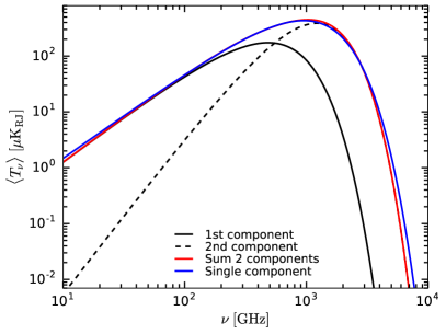
   Figure 1: Frequency dependence of the mean dust temperature for the two-component model of Meisner and Finkbeiner (2015) (red solid line, individual components shown as black solid and dashed lines) and for the single MBB model of Planck Collaboration et al. (2015b) (blue solid line). Both models provide a good fit to the data for most of the frequency range typically covered by CMB experiments, and data at higher and lower frequencies would be necessary to distinguish them.

3. Thermal dust: the long-wavelength tail of the thermal emission by Galactic dust grains heated by stellar radiation is the main foreground source at frequencies larger than $\sim 100\,{\rm GHz}$. Furthermore, the alignment of non-spherical grains with the Galactic magnetic field generates linear polarization orthogonal to it and to the line of sight, thus making thermal dust arguably the most important contaminant for $B$-mode searches.

   The emission of thermal dust has been shown to be relatively well fit by a modified black-body spectrum (MBB) with a power-law emissivity Planck Collaboration et al. (2015b). In this work we have generated simulations of the thermal dust emission using a method similar to the one described above for synchrotron. As before, we use a template for the emission amplitude on large scales at a fixed frequency generated by PySM, on top of which small-scale fluctuations are added as a high-pass filtered Gaussian realization of a power-law power spectrum $C_{\ell}\propto\ell^{\alpha_{d}}$, with $\alpha_{d}=-2.3$, modulated by the normalized local mean of the large-scale template smoothed on scales $\theta_{\rm FWHM}=10^{\circ}$. This amplitude map is then extrapolated by PySM to different frequencies using templates for the spectral parameters of the modified black-body intensity (spectral index $\beta_{d}$ and dust temperature $\Theta_{d}$). The explicit model used here is then:

   $$T_{\rm dust}(\nu,\hat{\bf n})= \left[T_{\rm LS}(\nu_{0},\hat{\bf n})+\left(\frac{T_{10^{\circ}}(\hat{\bf n})}{\bar{T}_{10^{\circ}}}\right)^{\gamma}\,T_{\rm SS}(\hat{\bf n})\right]\times$$

   $$\left(\frac{\nu}{\nu_{0}}\right)^{\beta_{d}(\hat{\bf n})}\frac{B_{\nu}(\Theta_{d}(\hat{\bf n}))}{B_{\nu_{0}}(\Theta_{d}(\hat{\bf n}))},$$ (3)

   where $\gamma=1.5$ and

   $$B_{\nu}(\Theta)\equiv\frac{2h\nu^{3}}{c^{2}}\left[\exp\left(\frac{h\nu}{k\,\Theta}\right)-1\right]^{-1}$$ (4)

   is the black-body spectrum. We must note that, even though the amplitude of different foreground components should be spatially correlated, we have neglected this correlation on the small scales where we add power. The effect of this assumption should be irrelevant for the large-scale observables ($\ell\lesssim 100$) we are interested in.

   For intensity PySM uses the Commander templates for the amplitude and spectral parameters at $\nu_{0}=545\,{\rm GHz}$ Planck Collaboration et al. (2015b). In polarization, we use the Commander templates for the $Q$ and $U$ amplitudes at $\nu_{0}=353\,{\rm GHz}$, which are extrapolated to other frequencies using the same spectral parameter templates used for intensity. Note that this model is not completely realistic: the different alignment efficiency of different types of dust grains should induce a different frequency dependence in intensity and polarization, and there is evidence for this in the Planck data Planck Collaboration et al. (2015c) in terms of a global spectral index. However, there is no estimate to date of the spatial variation of the polarized dust spectral index, and therefore we adopt the model above in order to simulate this spatial variation.

   It has been noted in the literature Finkbeiner et al. (1999); Meisner and Finkbeiner (2015) that a two-component dust model, with independent spectral indices and dust temperatures for both components, provides a marginally better fit when combining the Planck and DIRBE data. Although the joint emission from these two components can be qualitatively fit by a single MBB spectrum (see Fig. 1), future experiments might be sensitive to the differences between both models. Therefore we have run a number of simulations using a two-component dust model. For this, in intensity PySM uses the amplitude and dust temperature templates provided by Meisner and Finkbeiner (2015), together with their best-fit parameters. The corresponding polarization templates at 353 GHz are then generated as:

   $$(Q,U)_{353}(\hat{\bf n})=p_{353}(\hat{\bf n})\,T_{353}^{2c}(\hat{\bf n})\,(\sin 2\gamma(\hat{\bf n}),\cos 2\gamma(\hat{\bf n})),$$ (5)

   where $T_{353}^{2c}$ is the predicted intensity of the two-component model at 353 GHz, and $p_{353}(\hat{\bf n})$ and $\gamma(\hat{\bf n})$ are maps of the polarized fraction and polarization angles at 353 GHz predicted by the best-fit Commander single-component dust model.

   It is worth noting that, even though by using this second model we have tried to explore departures from our fiducial single-component model, the actual nature of thermal dust emission could be significantly more complicated than either of them.

4. AME/Spinning dust. The rotation (as opposed to vibration) of dust grains can also produce microwave emission, and this process is believed to be behind the so-called “anomalous dust emission” (AME), most prominent at low frequencies. Although the level to which this component is polarized is not clear, a failure to account for it could bias the measurement of $r$ in $B$-mode searches, and for this reason we have run a few simulations including this effect.

   We use the AME templates provided in the PySM package. In intensity, the code uses the best-fit Commander AME model and templates Planck Collaboration et al. (2015b). This model allows for two spinning dust components with different amplitudes and spectral parameters. The model spectrum is computed using SpDust2 Ali-Haïmoud et al. (2009); Silsbee et al. (2011) for a cold neutral medium, and can be rigidly shifted in $\log(\nu)$ by varying the peak frequency parameter. The peak frequency of the first component varies spatially at degree scales in the range $\nu_{p1}(\hat{\bf n})\sim 19\pm 3$ GHz, but the second component is spatially constant at $\nu_{p2}=33$ GHz. These spectra are then used to extrapolate two templates at reference frequencies $\nu_{1},\nu_{2}=22.8,41.0$ GHz, which are also limited to degree-scale resolution. The model can be summarized as:

   $$T^{\rm AME}_{\nu}(\hat{\bf n})=T_{\nu_{1}}(\hat{\bf n})f_{\rm{\tt SpDust}}(\nu_{p1}(\hat{\bf n}),\nu)+T_{\nu_{2}}(\hat{\bf n})f_{\rm{\tt SpDust}}(\nu_{p2},\nu).$$ (6)

   The resulting total spectrum is much broader than those of the individual components, and peaks in the range $\sim 20-30$ GHz. It is stressed in Planck Collaboration et al. (2015b) that the second component is included only because a single component model left significant dust-correlated residuals. The use of a second component is therefore not physically motivated, but is a convenient fit to the data.

   In polarization, PySM uses a simple model based on assuming a constant polarized fraction $p_{\rm AME}$ and using the polarization angle $\gamma(\hat{\bf n})$ for thermal dust emission found at 353 GHz. Thus

   $$(Q,U)_{\nu}(\hat{\bf n})=p_{\rm AME}\,T^{\rm AME}_{\nu}(\hat{\bf n})\,(\sin 2\gamma(\hat{\bf n}),\cos 2\gamma(\hat{\bf n})).$$ (7)

   In our simulations we assumed a $2\%$ polarization fraction ($p_{\rm AME}=0.02$). Since there are physical reasons to expect that spinning dust should be almost unpolarized Draine and Hensley (2016), the model adopted here represents a conservative case. However note that other alternative models for AME, such as magnetic dust Draine and Lazarian (1999) could be significantly more polarized.

Table 1 lists all the different simulations that were used for this work, corresponding to different variations of the models quoted above, together with different choices of the experiment design as well as the foreground cleaning algorithm. We note that the results quoted in this paper correspond to those extracted from a single simulation for each combination of experiment, sky and noise model, sky area and foreground cleaning method. However, we verified that our main results, in terms of the final uncertainty on the tensor-to-scalar ratio depend very little on the particular realization used.

II.2 Experimental setups

Name	Frequencies (GHz)	RMS noise ($\mu{\rm K}_{\rm CMB}\,{\rm arcmin}/f_{\rm sky}^{1/2}$)
Stage-3	(28, 41, 90, 150, 230, 353)	(171, 152, 14.2, 8.9, 16.5, $24^{*}$)
Stage-4	(30, 40, 85, 95, 145, 155, 215, 270)	(29, 29, 4.7, 3.7, 3.5, 3.4, 5.2, 4.5)

Table 2: Specifications for representative CMB experiments. For S3 we use the target frequencies and noise levels of AdvACT Henderson et al. (2015) and scale them up by a factor of $\sqrt{2}$ assuming that only half of the survey will be devoted to B-mode searches. For S4, Buza and et al. (2016) choose a possible set of frequency channels in the atmospheric windows and noise levels designed to yield a map-level rms noise of $\sim 1\mu\text{K-arcmin}$ after foreground cleaning for $f_{\rm sky}=0.1$ Buza and et al. (2016); S4 collaboration and et al. (2016). Here the assumption is that the first three atmospheric windows would be covered by two different frequency channels. Note that in both cases the quoted noise levels are given in intensity, in antenna temperature units and for a full-sky experiment. When studying different sky areas the noise levels are therefore scaled with $\sqrt{f_{\rm sky}}$ accordingly. ^∗The only exception to this is the 353 GHz frequency channel for S3, which corresponds to the Planck 353 GHz map, and therefore does not scale with sky area (see Section III.1 for further details). The noise levels above are quoted in intensity, and assume that the noise levels in $Q$ and $U$ will be a factor $\sqrt{2}$ larger.

The previous generation of ground-based CMB experiments, such as ACTPol Naess et al. (2014) and SPT-Pol Keisler et al. (2015) have now been upgraded, or are being upgraded into so-called Stage-3 (S3) facilities, including AdvACT Henderson et al. (2015) and SPT-3G Benson et al. (2014). Looking ahead, S3 experiments will be superseded by a Stage 4 (S4) experiment, likely to be built by combining the observing power of different ground-based facilities, with similar potential for wide sky coverage and significantly lower noise levels.

Here we have considered two different experimental setups, corresponding to a Stage-3 AdvACT-like experiment, characterised by a $1.4$ arcmin. beam and $\sim 8\,\mu K\,{\rm arcmin}$ rms noise (for a nominal $f_{\rm sky}=0.4$ sky coverage), and a future S4-like experiment, with roughly eight times lower noise. The frequency channels and noise levels used in both cases are summarized in Table 2. For the S4-like experiment, the specifications are not yet well defined so we use map depths estimated by Buza and et al. (2016), derived by scaling the achieved performance of the BICEP2/Keck experiments BICEP2 Collaboration et al. (2016). Note that, in the case of S3, we have also added the Planck 353 GHz data, which should help remove thermal dust. In the rest of this work, whenever we study the effects of using a reduced sky fraction, these noise levels were scaled down with $\sqrt{f_{\rm sky}}$ accordingly, assuming a constant observation time. In terms of defining the observable sky fraction, we will also assume that both experiments are located in the southern hemisphere.

Each simulation consists of a set of $I,\,Q$ and $U$ maps in the frequency bands listed in Table 2. These maps were generated using the HEALPix pixelization scheme Górski et al. (2005) with resolution parameter $N_{\rm side}=256$, enough for detecting the large-scale $B$-mode signal, and instrumental Gaussian noise was added to every map.

Atmospheric correlated noise is an important concern for ground-based experiments, in particular regarding large-scale observables such as primordial $B-$modes. For this reason, we have studied the effects of correlated noise by simulating the noise maps as Gaussian realizations of a power spectrum $N_{\ell}$ consisting of an uncorrelated and a correlated, power-law-like component:

$$N_{\ell}=\sigma_{N}^{2}\,\left[1+\left(\frac{\ell}{\ell_{\rm knee}}\right)^{\gamma}\right],$$ (8)

where $\sigma_{N}^{2}$ is the noise variance per steradian (given by the white noise levels shown in Table 2) and $\gamma=-1.9$. The parameter $\ell_{\rm knee}$ determines the scale below which the correlated component dominates, and we have studied the cases $\ell_{\rm knee}=0,\,50$ and 100, where the first case corresponds to purely white noise. By default we will report on the results with $\ell_{\rm knee}=0$, and we will analyze the effects of correlated noise in Section III.3.

The value of the power-law index was chosen to roughly mimic the noise power spectrum achieved by the BICEP2/Keck experiments BICEP2 Collaboration et al. (2016), and we assume the same shape for the noise power spectrum in intensity and polarization. The actual noise properties of specific experiments, however, will depend on a number of factors, such as atmospheric properties, instrumental specifications including modulation method, or survey strategy. We do not study these details further in this paper.

II.3 Map-based component separation

In order to separate the different components that make up the total sky emission we have adopted here a map-based Bayesian scheme Eriksen et al. (2004, 2008); Dunkley et al. (2009); Stompor et al. (2009); Remazeilles et al. (2016). An advantage of map-based methods over power-spectrum-based foreground cleaning (e.g. BICEP2/Keck and Planck Collaborations et al. (2015)) is that the effect of spatially-varying foreground spectra can be taken into account, thus avoiding potential biases on large-scales. The advantage of Bayesian methods over blind methods such as the widely used internal linear combination method (ILC) Hinshaw et al. (2007), is that the resulting CMB maps are closer to optimal in terms of signal-to-noise ratio, and that the foreground uncertainties can be propagated consistently. On the other hand, the success of Bayesian methods relies on the goodness of the models adopted to describe the different components. We will discuss these differences further in Section III.4.

II.3.1 Description of the model

In this method, the combined sky emission is modelled as a sum of several components with different frequency dependences. Let us consider a sky map with $N_{\theta}$ pixels, $N_{p}$ polarization channels (e.g. $T,\,Q,\,U$), and $N_{\nu}$ frequency bands. A model containing $N_{c}$ components can then be written, in general, as:

$${\bf d}=\hat{F}\,{\bf T}+{\bf n},$$ (9)

where

• ${\bf d}$ is the data, written as a vector of $N_{\theta}\times N_{p}\times N_{\nu}$ elements.

• ${\bf n}$ is the instrumental noise, also with $N_{\theta}\times N_{p}\times N_{\nu}$ elements.

• ${\bf T}$ is a vector with $N_{\theta}\times N_{p}\times N_{c}$ elements containing the amplitudes of the different components.

• $\hat{F}$ is a $(N_{\theta}\times N_{p}\times N_{\nu})\times(N_{\theta}\times N_{p}\times N_{c})$ matrix containing the spectral dependence of the different components, with the form:

  $$F_{(i^{\prime}\,p^{\prime}\,\nu),(i\,p\,a)}\equiv f_{a}(\nu;{\bf b}_{a}^{p}(i))\,\delta_{i,i^{\prime}}\delta_{p,p^{\prime}}.$$ (10)

  Here $i,\,p,\,\nu$ and $a$ label the different angular pixels, polarization channels, frequency bands and sky components respectively, and ${\bf b}$ is a set of spectral parameters. In our case these are the synchrotron spectral index and the dust temperature and spectral index. Explicitly, for the three components considered here, $\hat{F}$ is

  $${\rm CMB} :\,f_{C}(\nu)=\left.\frac{dB_{\nu}(\Theta)}{d\Theta}\right|_{\Theta=\Theta_{\rm CMB}},$$ (11)

  $${\rm synch.} :\,f_{s}(\nu;\beta_{s})=\left(\frac{\nu}{\nu_{0}^{s}}\right)^{\beta_{s}}$$ (12)

  $${\rm dust.} :\,f_{d}(\nu;\beta_{d},\Theta_{d})=\left(\frac{\nu}{\nu_{0}^{d}}\right)^{\beta_{d}}\frac{B_{\nu}(\Theta_{d})}{B_{\nu_{0}^{d}}(\Theta_{d})}.$$ (13)

The method then consists of sampling the distribution of the free parameters of the model, which are given by:

• Amplitudes, ${\bf T}$. $3\times N_{p}\times N_{\theta}$ of them.

• Spectral indices, ${\bf b}^{p}_{a}$. We will assume independent spectral indices in intensity and polarization, but a common index for $Q$ and $U$. Furthermore, we will make the simplifying assumption that spectral indices vary only over pixels larger than our base resolution. Labelling the total number of such pixels as $N^{\prime}_{\theta}<N_{\theta}$ we then have $2\times 3\times N^{\prime}_{\theta}$ spectral parameters.

We can compare the total number of parameters of the model, $N_{\rm par}=3\times N_{p}\times N_{\theta}+6\times N^{\prime}_{\theta}$, with the total number of data points, $N_{\rm data}=N_{p}\times N_{\nu}\times N_{\theta}$, to see that we need $N_{\nu}>3$ frequency channels to prevent the system from becoming overparametrized.

Using Bayes’ Theorem, we can write the posterior distribution for the model parameters as

$$p({\bf T},{\bf b}|{\bf d})\propto p_{l}({\bf d}|{\bf T},{\bf b})\,p_{p}({\bf T},{\bf b}),$$ (14)

where $p_{p}$ is the prior distribution for the parameters (which we will discuss later on) and $p_{l}$ is the Gaussian likelihood, given by

$$-2\log p_{l}({\bf d}|{\bf T},{\bf b})=C+\left[{\bf d}-\hat{F}\,{\bf T}\right]^{T}\hat{N}^{-1}\left[{\bf d}-\hat{F}\,{\bf T}\right].$$ (15)

Here $\hat{N}\equiv\langle{\bf n}\,{\bf n}^{T}\rangle$ is the noise covariance matrix, which we assume to be uncorrelated between frequency and polarization channels

$$N_{(i\,p\,\nu),(i^{\prime}\,p^{\prime}\,\nu^{\prime})}=N_{i,i^{\prime}}^{p\nu}\delta_{pp^{\prime}}\delta_{\nu\nu^{\prime}}.$$ (16)

In reality, instrumental and atmospheric effects will induce correlations between these channels. Here we will further assume, for simplicity, that the noise covariance is white, so that

$$(\hat{N}^{-1})_{(i\,p\,\nu),(i^{\prime}\,p^{\prime}\,\nu^{\prime})}=\sigma_{\nu,p}^{-2}\delta_{ii^{\prime}}\delta_{pp^{\prime}}\delta_{\nu\nu^{\prime}},$$ (17)

where $\sigma_{\nu,p}^{2}$ is the per-pixel noise variance.

Note that, by assuming uncorrelated noise, the posterior distribution can be written as a product of distributions for the individual large pixels over which the spectral indices are allowed to vary. This greatly simplifies the task of sampling the amplitude and spectral parameters, but will in general not be a valid assumption in the presence of atmospheric noise for ground-based experiments. Nevertheless, even in the presence of spatially correlated noise, which we study in the subsequent sections, this assumption should not introduce a bias in the final component-separated maps as long as the different frequency channels are appropriately weighted according to their overall noise variance. The variance of the output maps, however, will be sub-optimal; in the analysis of real data the noise correlations would be included.

Note also that the logarithm of the posterior is a quadratic function of the amplitudes ${\bf T}$ (assuming that the prior on ${\bf T}$ takes a Gaussian form). We take advantage of this property implementing two different methods to carry out the sampling. First, the amplitudes can be directly sampled (with a $100\%$ acceptance rate) as Gaussian random fields separately from the spectral index using Gibbs sampling methods as in e.g. Eriksen et al. (2008); Dunkley et al. (2009); Armitage-Caplan et al. (2011). Secondly, it is possible to marginalize over the amplitudes analytically, and thus sample only the spectral indices from their marginal distribution. The latter method significantly improves the performance of the algorithm. We give further details about the advantages and implementation of these methods in Appendix A.

II.3.2 Priors

In this work we imposed loose Gaussian priors on the spectral parameters, with $\beta_{s}=-3\pm 0.5$, $\beta_{d}=1.54\pm 0.5$ and $\Theta_{d}=20\pm 0.5\,{\rm K}$. The width of these priors is large enough to avoid biases in the final maps, and we verified that they seldom drive the posterior distribution. Besides these, we included a “volume prior” designed to take into account the volume of likelihood space for non-linear parameters. This is described in detail in Appendix B, and is equivalent to the widely used Jeffreys prior for the spectral parameters Eriksen et al. (2008).

II.4 Measuring $r$

After foreground cleaning we are left with a map of the mean and variance of the CMB intensity and polarization with fully propagated foreground uncertainties. From this map we determine $r$ and its uncertainty using a power-spectrum based likelihood, assuming that the $BB$ bandpowers are Gaussianly distributed:

$$-2\ln{\cal L}(r,A_{L})={\rm const.}+\sum_{k,k^{\prime}}\left[\hat{B}_{k}-B^{\rm th}_{k}(r,A_{L})\right]\left(\Sigma^{-1}\right)^{-1}_{kk^{\prime}}\left[\hat{B}_{k^{\prime}}-B^{\rm th}_{k^{\prime}}(r,A_{L})\right],$$ (18)

where $\hat{B}_{k}\equiv\sum_{\ell}W^{k}_{\ell}\hat{C}^{\rm BB}_{\ell}$ and $B^{\rm th}_{k}$ are the measured and model $B$-mode bandpowers, and $\Sigma_{kk^{\prime}}$ is the covariance matrix of $\hat{B}_{k}$. We model the $B$-mode power spectrum in terms of a primordial and a lensing component, each multiplied by a free amplitude parameter ($r$ and $A_{L}$ respectively):

$$C^{\rm th}_{\ell}=r\,C^{\rm prim}_{\ell}(r=1)+A_{L}\,C^{\rm lens}_{\ell}.$$ (19)

Here the primordial and lensing templates are held fixed to fiducial $\Lambda$CDM values.

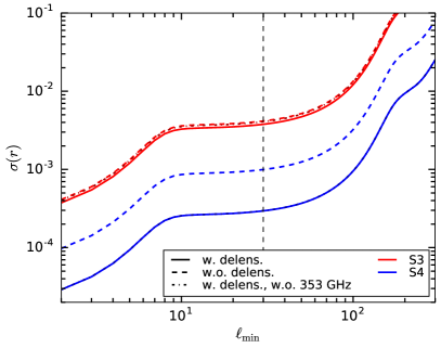
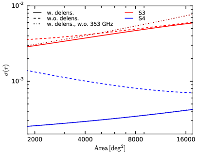
Figure 2: Left panel: 68% uncertainty levels on $r$ as a function of the minimum multipole included in the analysis for a fiducial sky area of $4000\,{\rm deg}^{2}$. Red and blue lines correspond to S3 and S4 respectively. Solid (dashed) lines show the results with (without) delensing, and the dot-dashed lines correspond to the same experiments after excluding the Planck 353 GHz channel. Right: uncertainty on $r$ as a function of sky area for a fixed observation time and for a fiducial $\ell_{\rm min}=30$. The Figure uses the same color code and line styles used in the left panel. Note that, while the Planck 353 GHz channel could help reduce the final uncertainty on $r$ for S3, especially for larger sky areas (higher noise), it is irrelevant for S4, given its lower noise levels (the blue solid and dot-dashed lines are indistinguishable).

Note that the power spectrum bandpowers are not Gaussianly distributed. However, at sufficiently large $\ell$, the central limit theorem guarantees that their distribution can be well approximated as such, since they are determined by averaging over all $|a_{\ell m}|$’s corresponding to the same $\ell$. Since many ground-based experiments are expected to be limited by atmosphere-related systematic effects on scales $\ell\lesssim 30$, using this approximation is justified.

Since ground-based observations from a single site can not fully cover the celestial sphere and, in any case, Galactic foregrounds prevent a clean measurement of primordial $B$-modes on the full sky, the angular power spectrum must be computed in the presence of a sky mask. There are several approaches to this problem in the literature, which range from the optimal approaches of the maximum likelihood estimator or the minimum-variance quadratic estimator Tegmark (1997) to the minimal approach of pseudo-$C_{\ell}$ estimators Hivon et al. (2002). The latter approach should be only marginally non-optimal for simple masks and non-steep power spectra (which is the case for $C_{\ell}^{BB}$), and therefore has been our method of choice for this work.

However, the use of pseudo-$C_{\ell}$ codes for polarized signals (or, in general, any spin-2 field) is complicated by the fact that a straightforward implementation of the method will give rise to a non-negligible contamination of $E$ into $B$ in the variance of the estimator. Since the CMB $E$-mode signal is much larger than the $B$-modes, this effect can make the pseudo-$C_{\ell}$ estimator severely sub-optimal. This problem can be solved by designing a pure-$B$ pseudo-$C_{\ell}$ estimator Smith (2006), which requires a non-trivial apodization around the edges of the mask. Since the aim of this paper is to assess the effect of foregrounds on the measurement of primordial $B$-modes, rather than the complications of power-spectrum estimation, we sidestep this problem by taking the following steps in each simulation:

1. Clean the foregrounds on the full sky.

2. Rotate the foreground-cleaned maps from $(T,Q,U)$ into the (pseudo) scalars $(T,E,B)$ on the full sky.

3. Apply the mask on the full-sky (pseudo)scalar maps.

4. Run a spin-0 pseudo-$C_{\ell}$ algorithm on the masked $(T,E,B)$ maps.

Thus this process preserves the complications of cut-sky observations (increased sample variance, correlations between band powers) while mimicking an optimal measurement of the $B$-mode power spectrum. We note that this method will yield smaller error bars than are actually achievable in a realistic situation. We can estimate the magnitude of this effect by noting that, as reported in Ferté et al. (2013), the pure-$B$ pseudo-$C_{\ell}$ estimator yields errors that are at most a factor of $\sim 2$ larger than the theoretical $\propto f^{-1}_{\rm sky}$ expectation, while we estimate the standard deviation of our spin-0 pseudo-$C_{\ell}$ to be a factor of $\sim 1.3$ larger than this ideal case. Thus, the uncertainties in the $B$-mode power spectrum in a realistic scenario would be, assuming a sub-optimal pseudo-$C_{\ell}$ approach, at most a factor $\sim 1.5$ larger than those reported here.

The details of the pseudo-$C_{\ell}$ method have been widely described in the literature, and we only quote the main details here. We compute the $BB$ power spectrum in bandpowers, estimated from the power spectrum of the cut-sky anisotropies as

$$\hat{B}_{k}=\sum_{k^{\prime}}(\hat{M}^{-1})_{kk^{\prime}}\,\tilde{B}_{k^{\prime}},$$ (20)

where

$$\tilde{B}_{k}=\sum_{\ell}\frac{W^{k}_{\ell}}{2\ell+1}\sum_{m}|\tilde{B}_{\ell m}|^{2},$$ (21)

$\tilde{B}_{\ell m}$ are the spherical harmonic coefficients of the masked $B$-mode map and $\hat{M}$ is the cut-sky coupling matrix. The latter depends only on the mask applied to the data, and its analytic expression can be found in Hivon et al. (2002). For this work we have used top-hat bandpowers characterised by a width $\Delta\ell$:

$$W^{k}_{\ell}=\frac{1}{\Delta\ell}\Theta(\ell-\ell_{k})\Theta(\ell_{k}+\Delta\ell-\ell),$$ (22)

where $\Theta(x)$ is the Heavyside function.

We avoid the problem of noise bias by using only cross-correlations between simulations run with the same CMB signal but different noise realizations. This mimics the usual approach of cross correlating splits of the full data in CMB experiments. Finally, for each simulation we compute the covariance matrix of the bandpowers $\Sigma_{k,k^{\prime}}$ from 1000 Gaussian realizations of the signal and noise $BB$ power spectrum measured from the two simulations. These realizations were cut using the same mask used in the analysis of the simulations, and therefore we fully account for possible non-zero correlations between bandpowers.

III Results

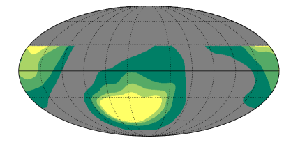
Figure 3: Sky masks used in the analysis, corresponding to the cleanest 2000, 4000, 8000 and 16000 ${\rm deg}^{2}$ of the sky accessible from Chile in terms of foreground contamination.

III.1 Fisher matrix forecasts

As a preliminary step, and in order to have an estimate of the most optimistic constraints on $r$ one can expect from our two model experiments, we have computed their corresponding Fisher forecast uncertainties. For this we assume global foreground spectral parameters $\beta_{s}=-3,\,\beta_{d}=1.54\,$ and $\Theta_{d}=20.9\,{\rm K}$, and a fiducial value of $r=0$. The foreground spectral parameters were held fixed, and thus these forecasts will yield the best possible uncertainties on $r$. Moreover, we assume a delensing factor $f_{\rm dl}$ related to the map noise level as described in Errard et al. (2016).

The left panel of Figure 2 shows the expected 1$\sigma$ constraints as a function of the minimum multipole $\ell_{\rm min}$ included in the analysis with and without delensing (solid and dashed lines respectively) for S3 and S4 (red and blue respectively). The results in the absence of the Planck 353 GHz map are shown as dot-dashed lines in both cases, and all curves assume a sky fraction $f_{\rm sky}=0.1$ for both experiments. As is evident from the Figure, while delensing is vital for S4 in order to significantly reduce the uncertainties on $r$, it is a lot less relevant for S3. Furthermore, the contribution of the 353 GHz map is irrelevant for S4, while it has a non-negligible impact for S3.

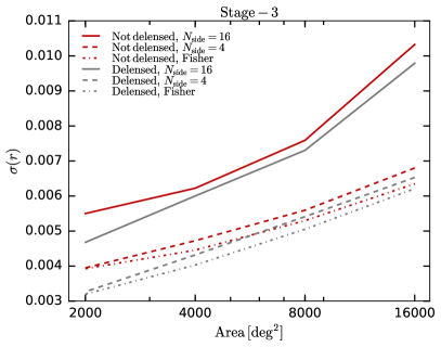
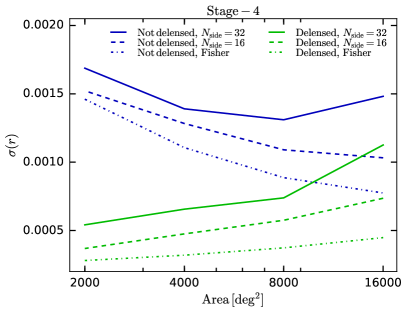
Figure 4: Simulated 68%-level uncertainties on $r$. Left: results for S3 with (without) delensing in gray (red). Results are shown for foregrounds cleaned assuming constant spectral indices on pixels of resolution $N_{\rm side}=4$ and 16 (solid and dashed lines respectively). Right: results for S4 with (without) delensing in green (blue), and for spectral indices assumed constant on pixels of size $N_{\rm side}=16$ and 32 (solid and dashed lines respectively). In both panels, the dot-dashed lines show the Fisher matrix forecasts, which assume fixed spectral indices.

Although the high-signal region $\ell_{\rm min}\lesssim 10$ caused by the reionization bump is likely inaccessible for ground-based experiments, the plateau between $\ell_{\rm min}\sim 10$ and $\ell_{\rm min}\sim 70$ can still be used to impose competitive constraints on $r$. Beyond $\ell_{\rm min}\sim 70$, the sensitivity to $r$ decreases sharply, and therefore it is important to cover the aforementioned plateau. In order to ensure that these large scales are sufficiently well sampled, we will only consider sky fractions $f_{\rm sky}\gtrsim 0.05$ for the rest of the analysis. The right panel of Fig. 2 shows the dependence of $\sigma(r)$ on $f_{\rm sky}$ for our fiducial value of $\ell_{\rm min}=30$.

III.2 Simulated forecasts

III.2.1 Foreground masks

In order to study the effects of foregrounds on $B$-mode searches as a function of sky fraction we have designed sky masks covering the cleanest 16000, 8000, 4000, and 2000 square degrees of the southern sky. We do so by first creating a map of the combined foreground emission by synchrotron and dust at 100 GHz smoothed on scales of $\sim 20^{\circ}$ and then selecting the connected regions in this map with the lowest foreground emission in $P\equiv\sqrt{Q^{2}+U^{2}}$. We further restrict these regions to lie in the range of declination ${\rm dec}\in[-75^{\circ},28^{\circ}]$. The resulting masks are shown in Fig. 3.

III.2.2 Results: fiducial foregrounds

We start by examining the fiducial simulations, with a single thermal dust component and without polarized AME. One of the free parameters of our method is the size of the large pixels, over which the spectral parameters are assumed to be constant. Smaller pixels allow us to capture the spatial variation of spectral indices more faithfully, at the cost of including a larger number of model parameters, which inevitably increases the final map-level noise (and consequently the uncertainty on $r$). We study the minimum resolution (in terms of the HEALPix $N_{\rm side}$ resolution parameter) needed to avoid biasing our $r$ measurement for the Stage-3 and Stage-4 experiments, given the fiducial foregrounds model adopted here. Figure 4 shows the $68\%$ uncertainty on $r$ for different resolutions for S3 and S4 (left and right panels respectively). The increase in $\sigma(r)$ caused by using more finely resolved spectral parameters is evident, and can be as large as a factor of $\sim 1.8$ for S3. We determined that $N_{\rm side}=4$, corresponding to an angular scale of $\sim 14^{\circ}$ is enough to avoid a bias in $r$ at the $1.5\sigma$ level (i.e. $\bar{r}<1.5\sigma(r)$) given the noise levels of S3, while at least $N_{\rm side}=16$ ($\sim 3.5^{\circ}$) was needed for S4 following the same criteria. Note that the resolution needed to fit for spectral parameters depends directly on the properties of the foregrounds, and therefore the values quoted here are specific to the simulations described in Section II.1.

Figure 4 also shows the effect of delensing in the final uncertainties. As we saw before, the improvement for S3 is only moderate, while the noise level of S4 makes the measurement of $r$ cosmic-variance limited in the absence of delensing. This can be clearly seen in the right panel of Fig. 4, not just as an increase in $\sigma(r)$ with respect to the delensed case, but also in the fact that, without delensing, a larger area is always preferred, in spite of its higher noise level. This trend reverts after delensing, when the measurement of $B$-modes becomes again noise-dominated. This is consistent with findings in e.g. Errard et al. (2016); Buza and et al. (2016).

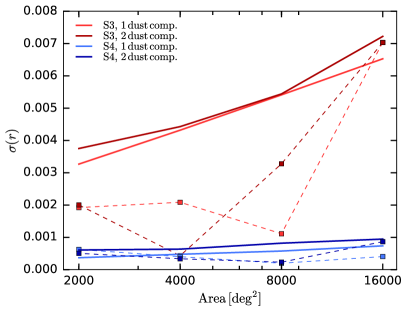
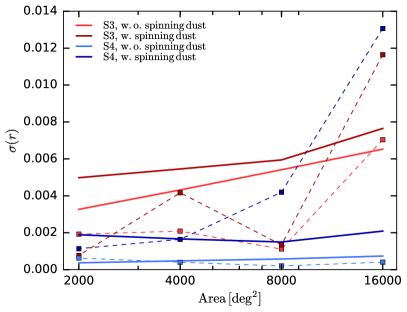
Figure 5: Simulated 68%-level uncertainties (solid lines) and measured value (dashed lines) of $r$ for foreground simulations that depart from our fiducial foreground model (used by the component separation code). Results are shown for S3 (red) and S4 (blue) for the fiducial and alternative foreground simulations (light and dark colors respectively). Left: results for 2 versus 1 independent thermal dust components. In this case we do not observe a significant ($>1.5\sigma$) bias on $r$. Right: results with and without $2\%$-polarized AME. The presence of this component would significantly bias the best-fit value of $r$ in the case of S4 if neglected at the component-separation stage, particularly for larger (more contaminated) sky areas.

Finally, Figure 4 also shows the value of $\sigma(r)$ predicted by the Fisher matrix approach described in the previous sections (which assumes fixed foreground spectral indices). The Fisher prediction is always more optimistic than our simulated results, although both are similar for S3 in the $N_{\rm side}=4$ case. This makes sense as, in the absence of spatially varying spectral parameters (i.e. in the limit $N_{\rm side}\rightarrow 0$), the Fisher prediction should be recovered.

In what follows, all results will be presented in the delensed case and for spectral parameters sampled in pixels of resolution $N_{\rm side}=4$ and $N_{\rm side}=16$ for S3 and S4 respectively.

III.2.3 Results: deviations from the fiducial model

Area (deg2)	$\chi^{2}/{\rm dof}-1$		${\rm PTE}(\chi^{2})$
	No AME	W. AME	No AME	W. AME
2000	$-5.91\times 10^{-4}$	$2.81\times 10^{-3}$	0.24	$0.099$
4000	$2.54\times 10^{-4}$	$2.31\times 10^{-3}$	0.18	$0.072$
8000	$1.02\times 10^{-3}$	$2.52\times 10^{-3}$	0.44	$0.013$
16000	$5.62\times 10^{-4}$	$1.93\times 10^{-3}$	0.61	$0.008$

Table 3: Values of the map $\chi^{2}$ for the mean amplitudes and spectral indices for S4 simulations with and without a polarized AME component, as well as the associated $p$-values. Although the overall $\chi^{2}$ per degree of freedom is close to 1 in all cases, the unaccounted-for AME component is associated with much smaller PTEs, which in the case of the higher sky areas would be a clear sign for missing components in the model used by the foreground cleaning algorithm. In this case, all spectral parameters were allowed to vary in pixels of resolution $N_{\rm side}=16$.

One of the drawbacks of Bayesian component separation methods is that specific models have to be assumed regarding the properties of the different components (e.g. frequency or spatial dependence). An incorrect modelling can therefore introduce biases that could potentially leak into the final cosmological parameters. In order to explore this possibility we have repeated the exercise described in the previous section on simulations containing foregrounds that are not described by the model used by our component separation code (i.e. single thermal dust component and power-law synchrotron). Specifically we generated simulations containing two thermal dust components, described by the model of Meisner and Finkbeiner (2015), and containing a $2\%$ polarized AME component.

The results are summarized in Figure 5, which shows the uncertainty on $r$ as a function of sky area as solid lines, together with its best-fit value as dashed lines. The left panel shows the results for the simulations with 2 dust components. Both for S3 and S4, the single-component model is able to fit well the joint emission of the 2 dust components, and no significant bias on $r$ is observed. The slight increase in $\sigma(r)$ with respect to the single-component model is caused by the different weighting of the different frequency maps needed to accommodate the spectral behavior of the 2-component model. We therefore conclude that the existence of a second dust component (with spectral properties compatible with current data) would not generate an important foreground bias in the measurement of primordial B-modes if unaccounted for.

The right panel of Fig. 5 shows the results in the presence of AME. As before, the bias on $r$ induced by the unaccounted-for AME is masked by the large noise levels of S3, and no significant bias can be appreciated. In the case of S4, however, we observe a dramatic biasing of $r$ caused by the presence of polarized AME, which lies above the $2\sigma$ level for the largest sky areas. Given such a large foreground bias, it is worth exploring whether the existence of an unmodelled component would have been detected at the foreground-cleaning stage. For this we studied the $\chi^{2}$ statistic of the mean amplitude and spectral parameter maps output by the component separation code. The results are shown in Table 3. For sky areas of 4000 sq deg or less, we find an acceptable probability for the incorrect model, with PTE of 7-10%, and a bias of about $1\sigma$ in the estimated value for $r$. Larger sky areas give a larger bias, but here the problem would be more likely identified as the PTE is only $\sim 1-2\%$. At this stage in the foreground cleaning, steps would be taken to account for an unidentified sky component. As noted by Remazeilles et al. (2016), however, there is no guarantee that a foreground bias in $r$ would be recognised by a map-space component separation algorithm, although other strategies, such as studying the isotropy of the recovered primordial $B$-modes would also help in identifying foreground residuals. Note also that, even though we find that the foreground bias for the smaller sky areas is below or around the $1\sigma$ error, statistical noise fluctuations could push it to higher values and induce a fake, low-significance detection of primordial $B$-modes. A more detailed study of polarized AME emission is therefore necessary in order to assess its potential impact on $B$-mode searches.

III.3 Results: correlated noise

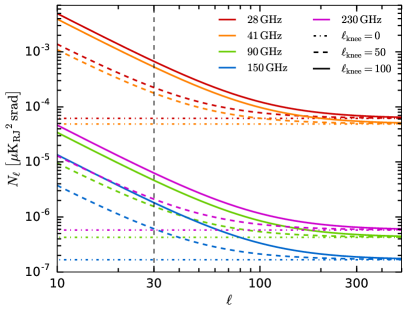
Figure 6: Noise curves assumed for S3 in the cases $\ell_{\rm knee}=100,\,50$ and 0 (solid, dashed and dot-dashed lines). The dashed vertical line marks the smallest multipole included in the analysis in all cases.

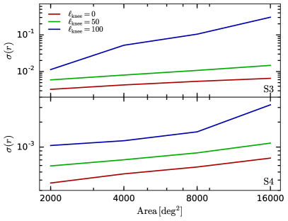
Figure 7: $68\%$ uncertainties on $r$ for S3 (upper panel) and S4 (lower panel) as a function of sky area and $\ell_{\rm knee}$, the scale above which the correlated noise component dominates. Results are shown for $\ell_{\rm knee}=0$ (uncorrelated noise, red lines), $\ell_{\rm knee}=50$ and $\ell_{\rm knee}=100$ (green and blue lines respectively). The sensitivity to $r$ degrades rapidly as the noise power on large scales increases.

So far we have assumed ideal experiments characterized by a Gaussian beam and purely white noise. However, one of the main disadvantages of ground-based CMB experiments is the effect of atmospheric emission and other contamination, which can be correlated (non-white) on large scales. Although the properties of this atmospheric noise depend on the geographical location of the experiment, it will generically affect any measurement of large-scale observables, such as the signature of primordial tensor perturbations. In polarization, the effects of atmospheric noise can be mitigated instrumentally through the use of half-wave plates (HWP), which efficiently separate the polarized sky signal from the unpolarized atmospheric noise. Therefore it is important to explore the impact of correlated atmospheric noise on the final uncertainties in order to translate the science requirements into instrument specifications.

In order to do this we repeated the analysis of our fiducial simulations (single thermal dust component and $0\%$ polarized AME) now including correlated noise. For this we used the model described in Section II.1, characterized by the parameter $\ell_{\rm knee}$, which determines the scale above which the noise becomes dominated by the correlated component. As shown in the left panel of Figure 2, the optimal range of scales for constraining B-modes accessible to ground-based experiments is $\ell\lesssim 100$, and therefore we studied the cases $\ell_{\rm knee}=50$ and $\ell_{\rm knee}=100$ (we will also show results for $\ell_{\rm knee}=0$, corresponding to the white-noise case studied before). Figure 6 shows examples of the noise power spectra used for S3 in this analysis. Note that, as before, in all cases we only used multipoles $\ell>30$ in the analysis.

The results are shown in Figure 7. Not surprisingly, the final constraints on $r$ are sensitive to the level of large-scale noise, with the uncertainties increasing by factors of $\sim 5$ and $\sim 3$ for S3 and S4 respectively between the $\ell_{\rm knee}=0$ and $\ell_{\rm knee}=100$ cases. Under the requirement that S3 and S4 experiments should be able to constrain the tensor-to-scalar ratio to better than $\sigma(r=0)\simeq 10^{-2}$ and $10^{-3}$ respectively for a $10\%$ sky fraction, we estimate that the lowest multipole below which large-scale atmospheric noise can be allowed to dominate should be approximately $\ell^{\rm max}_{\rm knee}\sim 50$.

III.4 Results: comparison with other methods

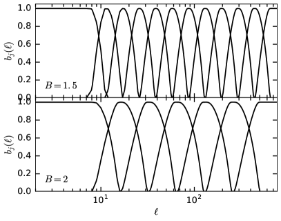
Figure 8: Window functions in harmonic space used to define the needlet basis used in the NILC algorithm. The upper and lower panels show the bands used for the $B$-adic parameter $B=1.5$ and $B=2$ respectively.

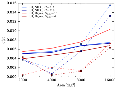
Figure 9: Results for S3 obtained using the Bayesian component separation code described in Section II.3 for spectral indices assumed constant in pixels of size $N_{\rm side}=4$ and 16 (light and dark red lines) compared with the results for a NILC algorithm defined using the $B$-adic mechanism for $B=1.5$ and 2 (light and dark blue lines). Solid lines show the 68%-level uncertainties, while dashed lines show the best-fit values of $r$ in all cases. Similar uncertainties are found with both methods, with the Bayesian approach being the most optimal one when only a small number of spectral indices are assumed free. A slight bias is found for the NILC algorithm for the largest sky area.

Many different methods have been used in the past to tackle the problem of component separation, and it would be interesting to study whether the results obtained here concerning the detectability of primordial $B$-modes are qualitatively universal across methods. To this end we have also implemented an independent version of the Needlet Internal Linear Combination algorithm (NILC, Delabrouille et al. (2009)) and compared its results with those of the Bayesian approach described above. A key difference between both methods is the complete model-independence of NILC, which does not assume a specific spectral dependence for any components other than the one we wish to separate (in this case the CMB). This should make NILC more robust to badly modelled foreground components, at the cost of sub-optimal final uncertainties. On the other hand, a key drawback of ILC methods is that the noise level of the output maps, as well as a potential bias in them, must be measured using simulations. However, for the purposes of verifying the validity of our results in terms of the expected uncertainties on the tensor-to-scala ratio, NILC is an appropriate alternative algorithm to compare with.

The details of the NILC algorithm have been thoroughly described in the literature Guilloux et al. (2007); Pietrobon et al. (2010), and we will only describe the method briefly here. It consists of three main steps:

• All the maps in the different frequency bands are first decomposed into a set of needlet coefficients $\psi_{j}(\hat{\bf n},\nu)$. These can be thought of as band-limited versions of the original maps in a set of multipole bands $b_{j}(\ell)$ characterized by a scale index $j$.

• For each scale, an internal linear combination of the different frequency channels that extracts the CMB component is determined for each pixel using information from all other pixels in a disc around it. The size of this disc is chosen such that the number of independent modes in the disc is large enough to ensure a reliable determination of the frequency-frequency covariance matrix.

• After applying the internal linear combination, we are left with a set of foreground-cleaned needlet coefficient $\psi^{c}_{j}(\hat{\bf n})$, which are then synthesized to generate the final cleaned CMB map.

In practice, we generalize this method to make use of polarized data by first transforming the input $(T,Q,U)$ maps at each frequency into the (pseudo)scalars $(T,E,B)$ and then applying the algorithm above to each component separately.

As described above, the needlet transforms needed to carry out the NILC algorithm are defined by the set of multipole bands $b_{j}(\ell)$. In our implementation we define these functions through the so-called $B$-adic mechanism Guilloux et al. (2007). In this case all the bands are defined in terms of a single function $h(x)$ with support in the range $x\in[1/B,B]$. The band functions are then defined as $b_{j}(\ell)=h(\ell/B^{j})$ and therefore have support in $\ell\in[B^{j-1},B^{j+1}]$. Thus, the spectral resolution of these bands is determined by the choice of $B>1$, and can be increased by choosing values of $B$ closer to $1$. The specific choice of $h(x)$ used in our implementation uses the guidelines of Pietrobon et al. (2010), and we studied the results for $B=1.5$ and 2. The corresponding $\ell$-bands for both cases are shown in Fig. 8.

The result of this exercise is shown in Figure 9 for S3 as a function of sky area. We see that, overall, we obtain uncertainties on $r$ that are somewhat larger than those obtained by the Bayesian component separation algorithm in the optimal $N_{\rm side}=4$ case. This reinforces our confidence in the expected uncertainties reported above. Furthermore, we observe a slight bias in the measured value of $r$ on the largest sky areas (still below $2\sigma$), caused by the inability of the NILC method to fully remove the large-scale foregrounds when more contaminated regions are included in the analysis.

IV Discussion

The detection of degree-scale CMB $B$-modes is one of the most important science cases for current and future CMB experiments, given the wealth of information contained in this observable. The detection and precise measurement of the $B$-mode power spectrum, however, is only achievable after accurately separating the cosmological signal from the large Galactic foregrounds in which it is immersed. In this work we have studied the ability of current (Stage-3) and future (Stage-4) ground-based experiments to recover the primordial $B$-mode signal in the presence of uncertain foregrounds. For this, we made use of realistic sky simulations processed through a data-analysis pipeline consisting of a Bayesian map-space component-separation code and a power-spectrum estimator. We thus try to subject the data to the analysis methods that would be used in a realistic setting, which allows us to fully propagate foreground uncertainties into the final constraints on the tensor-to-scalar ratio, as well as to identify possible biases in those constraints caused by an incorrect foreground modelling.

We find that accounting for highly resolved spectral indices causes a higher noise variance in the foreground-clean maps, which translates into larger final uncertainties on $r$. We therefore optimize the size of the resolution elements over which foreground spectral parameters are allowed to vary as a compromise between the size of the final error bars and the foreground bias associated with a poor representation of the spatial variation of these parameters. After doing that, we find that a Stage-3 AdvACT-like experiment should be able to constrain the tensor-to-scalar ratio to the level of $\sigma(r=0|{\rm S3})\simeq(4-6)\times 10^{-3}$, with S4 achieving sensitivities an order of magnitude better ($\sigma(r=0|{\rm S4})\simeq(4-6)\times 10^{-4}$). These estimates are within the context of the foreground models considered in this analysis, which are consistent with current data but do not necessarily capture all possible scenarios. They also assume full mode recovery for a small sky patch, and Gaussian noise.

Given the noise levels expected for S3, we find that it is always advantageous to push for deeper rather than wider observations if $r=0$, while the same is true for S4 only assuming optimal delensing levels. This is consistent with the findings of similar studies. We also find that delensing does not lead to a significant reduction in the forecast error on $r$ for S3, since the amplitude of the cosmic variance contribution from the lensing B-modes is comparable to the irreducible noise variance. Likewise, we observe that, given the noise levels of the 353 GHz Planck channel, its usefulness would be marginal for S3, and completely negligible for S4.

We have also studied the effect of atmospheric noise, modelling it as a correlated large-scale component that dominates on scales $\ell$ below some $\ell_{\rm knee}$. We find that large-scale non-white noise can dramatically affect the final constraints on $r$, especially if it dominates on scales $\ell\lesssim 100$, where most of the primordial $B$-mode signal is concentrated. We find that the uncertainties for purely white noise ($\ell_{\rm knee}=0$) grow by a factor of $\sim 3$ and $\sim 5$ for S4 and S3 respectively after assuming a large-scale correlated noise component dominating below $\ell_{\rm knee}=100$. Assuming that large-scale atmospheric noise can be kept under control, for instance through the use of half-wave plates, Stage-3 and Stage-4 experiments should still be able to measure the tensor-to-scalar ratio with accuracies $\sigma(r=0)=10^{-2}$ and $10^{-3}$ respectively, given the foreground models that we have considered. These measurements would directly translate into interesting constraints on inflationary theories.

Given the currently large uncertainties in the nature of polarized diffuse foregrounds, it is important to study departures from the fiducial synchrotron $+$ single thermal dust model, in order to explore the possible biases on $r$ caused by incorrect foreground modelling. To this extent we have considered simulations containing two different polarized thermal dust components and a polarized AME component at low frequencies (modelled as polarized spinning dust emission). We find that, given the noise levels of both S3 and S4, a single-component dust model should be able to describe the 2-component model sufficiently well, with no detectable foreground bias on $r$. On the other hand, a $2\%$ polarized AME component would induce, if unaccounted for, a significant bias on $r$ for S4, although its effects would be negligible given the larger noise levels of S3. This highlights the importance of future measurements of the polarized sky at low frequencies (by e.g. Rubiño-Martín et al. (2010); King et al. (2010)) in order to reduce our current uncertainties on the impact of polarized AME. There are also a variety of ways in which the true sky could be more complicated than any of the models we have considered here, and this will be the subject of future studies.

It is also important to note that there are a number of potential sources of instrumental systematic uncertainties that we have not considered in this paper, such as temperature-to-polarization leakage, beam asymmetries or ground and scan-synchronous pick-up, which could impact the final constraints on $r$. In future work we also anticipate comparing forecasts for a given S4-type experimental configuration using our methods, with the methods described in Errard et al. (2016); Buza and et al. (2016) as the definition of S4 is refined.

In order to obtain reliable constraints on the amplitude of large-scale $B$-mode fluctuations with future sensitive ground-based facilities, large efforts are needed both in understanding the physics of diffuse polarized Galactic foreground and in designing experiments and data analysis methods able to separate these foregrounds from the cosmological CMB signal. To this extent, map-based component separation methods are able to consistently propagate foreground uncertainties caused by spatially varying spectral parameters, and, as we have shown, can provide clear diagnostics of incomplete foreground cleaning. These, together with suites of null tests aimed at identifying sources of astrophysical or instrumental systematic effects, provide a path towards placing robust constraints on the physics of the inflationary Universe.

Appendix A Sampling the posterior

Here we describe the strategies used to sample the posterior distribution introduced in Section II.3.

A.1 Sampling the posterior I: Gibbs sampling

The Gibbs sampling algorithm tries to solve the problem of sampling from a multivariate distribution by alternatively sampling from the distribution of the different parameters (or sets of parameters) conditional on the previous iterations of the rest. In our case, let ${\bf T}_{i}$, ${\bf b}_{i}$ denote the $i$-th sample of the amplitudes and spectral indices. We then draw the $(i+1)$-th sample as

$${\bf T}_{i+1}\leftarrow p_{l}({\bf T}|{\bf d},{\bf b}_{i})\propto p({\bf d}|{\bf T},{\bf b}_{i})\,p_{p}({\bf T}),$$ (23)

$${\bf b}_{i+1}\leftarrow p_{l}({\bf b}|{\bf d},{\bf T}_{i+1})\propto p({\bf d}|{\bf T}_{i+1},{\bf b})\,p_{p}({\bf b})$$ (24)

The advantage of this method is that, since the amplitudes are Gaussianly distributed, they can be sampled analytically with a 100% acceptance ratio, thus gaining an enormous speed-up factor with respect to a naive Monte Carlo sampling of the individual parameters.

Explicitly, the conditional distribution for ${\bf T}$ assuming no prior on the amplitudes can be written as

$$p({\bf T}|{\bf d},{\bf b})\propto\exp\left[-\frac{1}{2}\left({\bf T}-\bar{\bf T}\right)^{T}\hat{N}_{T}^{-1}\left({\bf T}-\bar{\bf T}\right)\right],$$ (25)

where

$$\hat{N}_{T}^{-1}=\hat{F}^{T}\hat{N}^{-1}\hat{F},\hskip 12.0pt\bar{\bf T}=\hat{N}_{T}\,\left(\hat{F}^{T}\hat{N}^{-1}{\bf d}\right).$$ (26)

Samples from Eq. 25 can then be easily drawn as

$${\bf T}_{i}=\bar{\bf T}+\hat{L}^{-1}\,{\bf u},$$ (27)

where ${\bf u}$ is an uncorrelated, unit-variance Gaussian random vector, and $\hat{L}$ is the Choleski decomposition of $\hat{N}_{T}^{-1}$ (i.e. $\hat{N}_{T}^{-1}=\hat{L}^{T}\hat{L}$). The spectral indices are then sampled jointly using a multi-dimensional Monte-Carlo Markov Chain (MCMC) Metropolis-Hastings algorithm.

A.2 Sampling the posterior II: marginalising over amplitudes

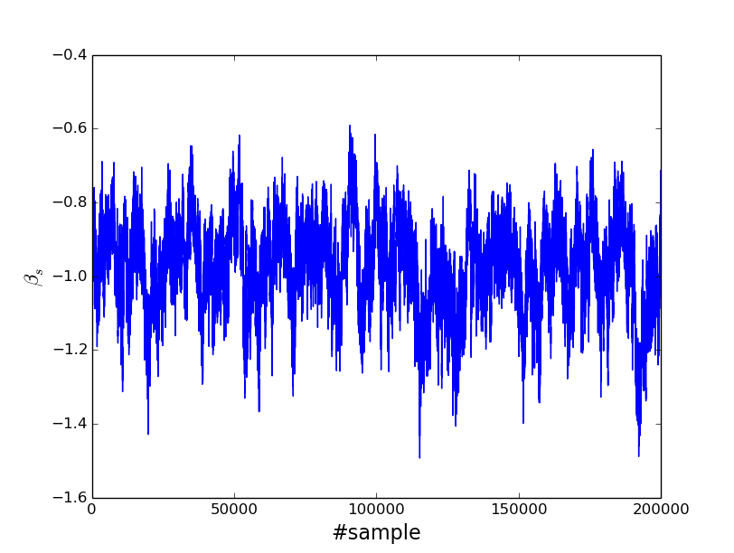
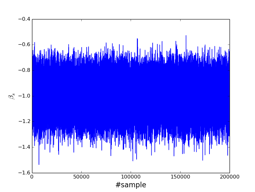
Figure 10: Left panel: MCMC chain for $\beta_{s}$ in the case where amplitudes are sampled via Gibbs sampling. Right panel: MCMC chain for $\beta_{s}$ for indices sampled directly from the marginal distribution.

Since the amplitudes ${\bf T}$ are Gaussianly distributed, it is also possible to analytically marginalize over them to obtain the marginal distribution for the spectral indices. As noted above, the likelihood $p_{l}({\bf d}|{\bf T},{\bf b})$ in Eq. 15 can be written as in Eq. 25. Writing the ${\bf b}$-dependent proportionality constant explicitly we obtain:

$$p({\bf T},{\bf b}|{\bf d})\propto \frac{\exp\left[-\frac{1}{2}\left({\bf T}-\bar{\bf T}\right)^{T}\hat{N}_{T}^{-1}\left({\bf T}-\bar{\bf T}\right)^{T}\right]}{\sqrt{{\rm det}(\hat{N}_{T})}}\times$$

$$\sqrt{{\rm det}(\hat{N}_{T})}\exp\left[\frac{1}{2}\bar{\bf T}^{T}\hat{N}_{T}^{-1}\bar{\bf T}\right]p_{p}({\bf b}).$$ (28)

Integrating this equation over the amplitudes we see that the first term integrates out to a constant factor, and thus we obtain the marginal distribution for the spectral indices:

$$p({\bf b}|{\bf d})\propto\sqrt{{\rm det}(\hat{N}_{T})}\exp\left[\frac{1}{2}\bar{\bf T}^{T}\hat{N}_{T}^{-1}\bar{\bf T}\right]p_{p}({\bf b}).$$ (29)

Why is it relevant to go through all this trouble? Ultimately we are interested in the moments of the distribution of the amplitude of the CMB component. The expectation value for any function of the amplitudes can be computed as an integral over the marginal distribution:

$$\langle g({\bf T})|{\bf d}\rangle =\int d{\bf T}d{\bf b}\,g({\bf T})p({\bf T},{\bf b}|{\bf d}),$$ (30)

$$=\int d{\bf b}\,\langle g({\bf T})|{\bf b},{\bf d}\rangle\,p({\bf b}|{\bf d})$$ (31)

Since the conditional distribution $p({\bf T}|{\bf d},{\bf b})$ is Gaussian, it is completely defined by the first 2 moments of the distribution:

$$\langle{\bf T}|{\bf d},{\bf b}\rangle=\bar{\bf T},\hskip 12.0pt\langle({\bf T}-\bar{\bf T})({\bf T}-\bar{\bf T})^{T}|{\bf d},{\bf b}\rangle=\hat{N}_{T},$$ (32)

which can be computed analytically for any value of ${\bf b}$. Thus we can compute the marginalized mean and covariance of the amplitudes by sampling only the spectral indices from their marginal posterior in Eq. 29 and computing the analytical conditional mean and covariance for each sample.

It is easy to see how doing this would improve the performance of the method. By skipping the intermediate sampling of the amplitudes (Eq. 23), we reduce the correlation length of the the MCMC chains for ${\bf b}$, and fewer samples are needed to cover the posterior. Figure 10 shows a Monte-Carlo chain for $\beta_{s}$ in the full Gibbs-sampling scheme of the previous section (left) and sampling directly from the marginal distribution (right).

Appendix B Volume prior for spectral parameters

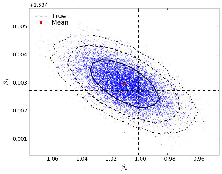
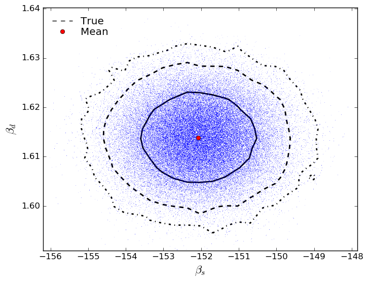
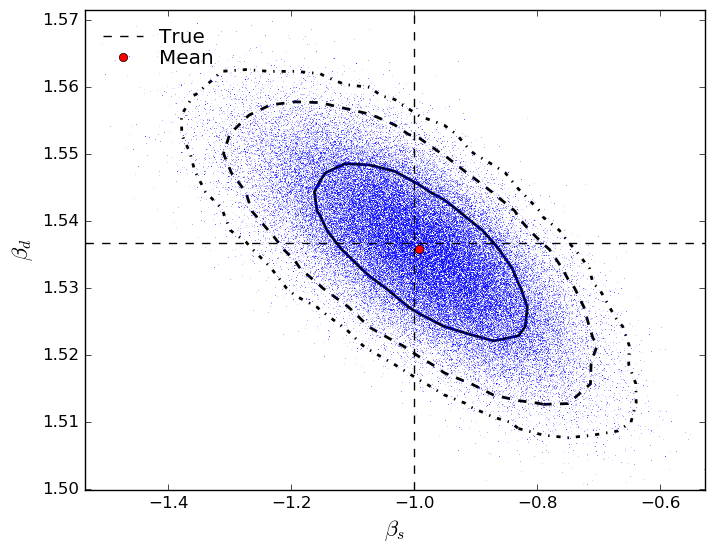
Figure 11: Upper left panel: contour plots ($1,2,3\sigma$ - solid, dashed and dot-dashed lines), mean value (red circle) and true value (dashed lines) of the dust and synchrotron spectral indices for a high-SNR region without cancelling the volume factor. The posterior mean is more than 3-sigmas away from the true input value. Upper right panel: same plot after cancelling the volume prior. The true value lies within $2\sigma$ of the posterior mean. The lower panels show the same for a low-SNR region.

As has been noted in the literature, when dealing with non-linear parameters, a flat prior is not necessarily appropriate to describe quantitatively our ignorance about their value. This can be easily ilustrated using the results of Appendix 10.

Consider first the case of a noise-dominated map, where we can approximate the data as being completely made up of noise. In that case, the expectation value of the exponent in Eq. 29 is given by:

$$\left\langle\bar{\bf T}\hat{N}_{T}^{-1}\bar{\bf T}\right\rangle={\rm Tr}\left[\hat{N}_{T}\hat{F}^{T}\hat{N}^{-1}\langle{\bf d}{\bf d}^{T}\rangle\hat{N}^{-1}\hat{F}\right]=N_{A},$$ (33)

where $N_{A}$ is the number of amplitudes. Thus, in this regime, the posterior for the spectral parameters ${\bf b}$ is dominated by the prefactor $\sqrt{|\hat{N}_{T}|}$. In the simplified case where the only component is synchrotron, and in the absence of polarized channels, this volume factor is given by:

$$\sqrt{|\hat{N}_{T}|}\propto\left[\sum_{\nu}\left(\frac{\nu}{\nu_{0}^{s}}\right)^{2\beta_{s}}\frac{1}{\sigma_{\nu}^{2}}\right]^{-1/2},$$ (34)

which becomes arbitrarily large for $\beta_{s}\rightarrow-\infty$. This result makes qualitative sense: in the absence of data, we must cancel the synchrotron component. This can be achieved by either having very small amplitudes or a very steep spectral index. Since a large $|\beta_{s}|$ would give rise to a negligible synchrotron component, even for very large amplitudes, this option covers a larger volume of the space of parameters.

However, is this behavior desirable? Presumably, we would expect that, in the absence of signal, the spectral indices would be completely unconstrained, or else dominated by the prior $p_{p}({\bf b})$. More importantly, since this volume factor does not depend on the data, could its presence bias our estimate of ${\bf b}$ in the case where the data contains a measurable amount of signal? This can be easily shown to be the case Eriksen et al. (2008). The upper panels of Figure 11 show the likelihood contours for the dust and synchrotron spectral indices in a simulated patch of the sky with relatively high signal to noise. The left and right panels present the result before and after cancelling the volume factor respectively. The dashed lines show the true values of the spectral indices, and the red circles correspond to the mean of the posterior. The presence of the volume factor biases the estimate of the spectral indices by more than $4\sigma$, and their true value is recovered within $1\sigma$ after accounting for it. The situation in a low-$S/N$ region is ilustrated in the lower panels of Fig. 11: even using a broad Gaussian prior with $\sigma_{\beta}\sim 1.$ centered on the true values of the spectral indices, the mean estimated indices are hundreds of $\sigma$s away from their true values. These, however, are well recovered after cancelling the volume factor and, as shown in the right panel of this Figure, their uncertainty is not dominated at all by the Gaussian prior.

These two undesirable features (i.e. the non-flat posterior for the spectral indices in the signal-less case, and the bias it entails) can be avoided by including a factor $|\hat{N}_{T}|^{-1/2}$ in our prior that exactly cancels the volume factor. This problem can also be solved by applying a Jeffreys prior, given by the square root of the Fisher information matrix Eriksen et al. (2008)

$$p_{\rm Jef}(\theta)\propto\sqrt{F_{\theta\theta}}=\sqrt{-\left\langle\frac{\partial^{2}\mathcal{L}}{\partial\theta^{2}}\right\rangle}.$$ (35)

Note however, that for the case of a power-law spectral index, this is given by

$$p_{\rm Jef}(\beta_{s})\propto\sqrt{\sum_{\nu}\left[\left(\frac{\nu}{\nu_{0}^{s}}\right)^{\beta_{s}}\frac{1}{\sigma_{v}}\ln\left(\frac{\nu}{\nu_{0}^{s}}\right)\right]^{2}},$$ (36)

which is equivalent to the volume prior $p_{\rm Vol}\equiv|\hat{N}_{T}|^{-1/2}$ defined by Eq. 34 except for the subdominant logarithmic term.

References

- Kamionkowski et al. (1997) M. Kamionkowski, A. Kosowsky, and A. Stebbins, Physical Review Letters 78, 2058 (1997), eprint astro-ph/9609132.
- Seljak and Zaldarriaga (1997) U. Seljak and M. Zaldarriaga, Physical Review Letters 78, 2054 (1997), eprint astro-ph/9609169.
- Zaldarriaga and Seljak (1998) M. Zaldarriaga and U. Seljak, Phys. Rev. D 58, 023003 (1998), eprint astro-ph/9803150.
- Lyth (1997) D. H. Lyth, Physical Review Letters 78, 1861 (1997), eprint hep-ph/9606387.
- The Polarbear Collaboration: P. A. R. Ade et al. (2014) The Polarbear Collaboration: P. A. R. Ade, Y. Akiba, A. E. Anthony, K. Arnold, M. Atlas, D. Barron, D. Boettger, J. Borrill, S. Chapman, Y. Chinone, et al., Astrophys. J. 794, 171 (2014), eprint 1403.2369.
- Keisler et al. (2015) R. Keisler, S. Hoover, N. Harrington, J. W. Henning, P. A. R. Ade, K. A. Aird, J. E. Austermann, J. A. Beall, A. N. Bender, B. A. Benson, et al., Astrophys. J. 807, 151 (2015), eprint 1503.02315.
- Naess et al. (2014) S. Naess, M. Hasselfield, J. McMahon, M. D. Niemack, G. E. Addison, P. A. R. Ade, R. Allison, M. Amiri, N. Battaglia, J. A. Beall, et al., JCAP 10, 007 (2014), eprint 1405.5524.
- BICEP2 Collaboration et al. (2014) BICEP2 Collaboration, P. A. R. Ade, R. W. Aikin, D. Barkats, S. J. Benton, C. A. Bischoff, J. J. Bock, J. A. Brevik, I. Buder, E. Bullock, et al., Physical Review Letters 112, 241101 (2014), eprint 1403.3985.
- BICEP2/Keck and Planck Collaborations et al. (2015) BICEP2/Keck and Planck Collaborations, P. A. R. Ade, N. Aghanim, Z. Ahmed, R. W. Aikin, K. D. Alexander, M. Arnaud, J. Aumont, C. Baccigalupi, A. J. Banday, et al., Physical Review Letters 114, 101301 (2015), eprint 1502.00612.
- Planck Collaboration et al. (2016) Planck Collaboration, R. Adam, P. A. R. Ade, N. Aghanim, M. Arnaud, J. Aumont, C. Baccigalupi, A. J. Banday, R. B. Barreiro, J. G. Bartlett, et al., A&A 586, A133 (2016), eprint 1409.5738.
- The COrE Collaboration et al. (2011) The COrE Collaboration, C. Armitage-Caplan, M. Avillez, D. Barbosa, A. Banday, N. Bartolo, R. Battye, J. Bernard, P. de Bernardis, S. Basak, et al., ArXiv e-prints (2011), eprint 1102.2181.
- Kogut et al. (2011) A. Kogut, D. J. Fixsen, D. T. Chuss, J. Dotson, E. Dwek, M. Halpern, G. F. Hinshaw, S. M. Meyer, S. H. Moseley, M. D. Seiffert, et al., JCAP 7, 025 (2011), eprint 1105.2044.
- Matsumura et al. (2014) T. Matsumura, Y. Akiba, J. Borrill, Y. Chinone, M. Dobbs, H. Fuke, A. Ghribi, M. Hasegawa, K. Hattori, M. Hattori, et al., Journal of Low Temperature Physics 176, 733 (2014), eprint 1311.2847.
- Fraisse et al. (2013) A. A. Fraisse, P. A. R. Ade, M. Amiri, S. J. Benton, J. J. Bock, J. R. Bond, J. A. Bonetti, S. Bryan, B. Burger, H. C. Chiang, et al., JCAP 4, 047 (2013), eprint 1106.3087.
- Remazeilles et al. (2016) M. Remazeilles, C. Dickinson, H. K. K. Eriksen, and I. K. Wehus, MNRAS 458, 2032 (2016), eprint 1509.04714.
- Errard et al. (2016) J. Errard, S. M. Feeney, H. V. Peiris, and A. H. Jaffe, JCAP 3, 052 (2016), eprint 1509.06770.
- Thorne et al. (2016) B. Thorne, D. Alonso, and J. Dunkley, ArXiv e-prints (2016), eprint In prep.
- Lewis et al. (2000) A. Lewis, A. Challinor, and A. Lasenby, Astrophys. J. 538, 473 (2000), eprint astro-ph/9911177.
- Planck Collaboration et al. (2015a) Planck Collaboration, P. A. R. Ade, N. Aghanim, M. Arnaud, M. Ashdown, J. Aumont, C. Baccigalupi, A. J. Banday, R. B. Barreiro, J. G. Bartlett, et al., ArXiv e-prints (2015a), eprint 1502.01589.
- Næss and Louis (2013) S. K. Næss and T. Louis, JCAP 9, 001 (2013), eprint 1307.0719.
- Knox and Song (2002) L. Knox and Y.-S. Song, Physical Review Letters 89, 011303 (2002), eprint astro-ph/0202286.
- Kesden et al. (2002) M. Kesden, A. Cooray, and M. Kamionkowski, Physical Review Letters 89, 011304 (2002), eprint astro-ph/0202434.
- Okamoto and Hu (2003) T. Okamoto and W. Hu, Phys. Rev. D 67, 083002 (2003), eprint astro-ph/0301031.
- Smith et al. (2012) K. M. Smith, D. Hanson, M. LoVerde, C. M. Hirata, and O. Zahn, JCAP 6, 014 (2012), eprint 1010.0048.
- Rybicki and Lightman (1986) G. B. Rybicki and A. P. Lightman, Radiative Processes in Astrophysics (1986).
- Delabrouille et al. (2013) J. Delabrouille, M. Betoule, J.-B. Melin, M.-A. Miville-Deschênes, J. Gonzalez-Nuevo, M. Le Jeune, G. Castex, G. de Zotti, S. Basak, M. Ashdown, et al., A&A 553, A96 (2013), eprint 1207.3675.
- Haslam et al. (1982) C. G. T. Haslam, C. J. Salter, H. Stoffel, and W. E. Wilson, A&AS 47, 1 (1982).
- Bennett et al. (2013) C. L. Bennett, D. Larson, J. L. Weiland, N. Jarosik, G. Hinshaw, N. Odegard, K. M. Smith, R. S. Hill, B. Gold, M. Halpern, et al., ApJS 208, 20 (2013), eprint 1212.5225.
- Miville-Deschênes et al. (2007) M.-A. Miville-Deschênes, G. Lagache, F. Boulanger, and J.-L. Puget, A&A 469, 595 (2007), eprint 0704.2175.
- Fuskeland et al. (2014) U. Fuskeland, I. K. Wehus, H. K. Eriksen, and S. K. Næss, Astrophys. J. 790, 104 (2014), eprint 1404.5323.
- Planck Collaboration et al. (2015b) Planck Collaboration, R. Adam, P. A. R. Ade, N. Aghanim, M. I. R. Alves, M. Arnaud, M. Ashdown, J. Aumont, C. Baccigalupi, A. J. Banday, et al., ArXiv e-prints (2015b), eprint 1502.01588.
- Meisner and Finkbeiner (2015) A. M. Meisner and D. P. Finkbeiner, Astrophys. J. 798, 88 (2015), eprint 1410.7523.
- Planck Collaboration et al. (2015c) Planck Collaboration, P. A. R. Ade, M. I. R. Alves, G. Aniano, C. Armitage-Caplan, M. Arnaud, F. Atrio-Barandela, J. Aumont, C. Baccigalupi, A. J. Banday, et al., A&A 576, A107 (2015c), eprint 1405.0874.
- Finkbeiner et al. (1999) D. P. Finkbeiner, M. Davis, and D. J. Schlegel, Astrophys. J. 524, 867 (1999), eprint astro-ph/9905128.
- Ali-Haïmoud et al. (2009) Y. Ali-Haïmoud, C. M. Hirata, and C. Dickinson, MNRAS 395, 1055 (2009), eprint 0812.2904.
- Silsbee et al. (2011) K. Silsbee, Y. Ali-Haïmoud, and C. M. Hirata, MNRAS 411, 2750 (2011), eprint 1003.4732.
- Draine and Hensley (2016) B. T. Draine and B. S. Hensley, ArXiv e-prints (2016), eprint 1605.06671.
- Draine and Lazarian (1999) B. T. Draine and A. Lazarian, Astrophys. J. 512, 740 (1999), eprint astro-ph/9807009.
- Henderson et al. (2015) S. W. Henderson, R. Allison, J. Austermann, T. Baildon, N. Battaglia, J. A. Beall, D. Becker, F. De Bernardis, J. R. Bond, E. Calabrese, et al., ArXiv e-prints (2015), eprint 1510.02809.
- Buza and et al. (2016) V. Buza and et al., In preparation (2016).
- S4 collaboration and et al. (2016) S4 collaboration and et al., In preparation (2016).
- Benson et al. (2014) B. A. Benson, P. A. R. Ade, Z. Ahmed, S. W. Allen, K. Arnold, J. E. Austermann, A. N. Bender, L. E. Bleem, J. E. Carlstrom, C. L. Chang, et al., in Millimeter, Submillimeter, and Far-Infrared Detectors and Instrumentation for Astronomy VII (2014), vol. 9153 of Proc. SPIE Int. Soc. Opt. Eng., p. 91531P, eprint 1407.2973.
- BICEP2 Collaboration et al. (2016) BICEP2 Collaboration, Keck Array Collaboration, P. A. R. Ade, Z. Ahmed, R. W. Aikin, K. D. Alexander, D. Barkats, S. J. Benton, C. A. Bischoff, J. J. Bock, et al., Physical Review Letters 116, 031302 (2016), eprint 1510.09217.
- Górski et al. (2005) K. M. Górski, E. Hivon, A. J. Banday, B. D. Wandelt, F. K. Hansen, M. Reinecke, and M. Bartelmann, Astrophys. J. 622, 759 (2005), eprint astro-ph/0409513.
- Eriksen et al. (2004) H. K. Eriksen, I. J. O’Dwyer, J. B. Jewell, B. D. Wandelt, D. L. Larson, K. M. Górski, S. Levin, A. J. Banday, and P. B. Lilje, ApJS 155, 227 (2004), eprint astro-ph/0407028.
- Eriksen et al. (2008) H. K. Eriksen, J. B. Jewell, C. Dickinson, A. J. Banday, K. M. Górski, and C. R. Lawrence, Astrophys. J. 676, 10-32 (2008), eprint 0709.1058.
- Dunkley et al. (2009) J. Dunkley, D. N. Spergel, E. Komatsu, G. Hinshaw, D. Larson, M. R. Nolta, N. Odegard, L. Page, C. L. Bennett, B. Gold, et al., Astrophys. J. 701, 1804 (2009), eprint 0811.4280.
- Stompor et al. (2009) R. Stompor, S. Leach, F. Stivoli, and C. Baccigalupi, MNRAS 392, 216 (2009), eprint 0804.2645.
- Hinshaw et al. (2007) G. Hinshaw, M. R. Nolta, C. L. Bennett, R. Bean, O. Doré, M. R. Greason, M. Halpern, R. S. Hill, N. Jarosik, A. Kogut, et al., ApJS 170, 288 (2007), eprint astro-ph/0603451.
- Armitage-Caplan et al. (2011) C. Armitage-Caplan, J. Dunkley, H. K. Eriksen, and C. Dickinson, MNRAS 418, 1498 (2011), eprint 1103.2554.
- Tegmark (1997) M. Tegmark, Phys. Rev. D 55, 5895 (1997), eprint astro-ph/9611174.
- Hivon et al. (2002) E. Hivon, K. M. Górski, C. B. Netterfield, B. P. Crill, S. Prunet, and F. Hansen, Astrophys. J. 567, 2 (2002), eprint astro-ph/0105302.
- Smith (2006) K. M. Smith, New Astronomy Review 50, 1025 (2006), eprint astro-ph/0608662.
- Ferté et al. (2013) A. Ferté, J. Grain, M. Tristram, and R. Stompor, Phys. Rev. D 88, 023524 (2013), eprint 1305.7441.
- Delabrouille et al. (2009) J. Delabrouille, J.-F. Cardoso, M. Le Jeune, M. Betoule, G. Fay, and F. Guilloux, A&A 493, 835 (2009), eprint 0807.0773.
- Guilloux et al. (2007) F. Guilloux, G. Fay, and J.-F. Cardoso, ArXiv e-prints (2007), eprint 0706.2598.
- Pietrobon et al. (2010) D. Pietrobon, A. Balbi, P. Cabella, and K. M. Gorski, Astrophys. J. 723, 1 (2010), eprint 1010.1371.
- Rubiño-Martín et al. (2010) J. A. Rubiño-Martín, R. Rebolo, M. Tucci, R. Génova-Santos, S. R. Hildebrandt, R. Hoyland, J. M. Herreros, F. Gómez-Reñasco, C. L. Caraballo, E. Martínez-González, et al., Astrophysics and Space Science Proceedings 14, 127 (2010), eprint 0810.3141.
- King et al. (2010) O. G. King, C. Copley, R. Davies, R. Davis, C. Dickinson, Y. A. Hafez, C. Holler, J. J. John, J. L. Jonas, M. E. Jones, et al., in Millimeter, Submillimeter, and Far-Infrared Detectors and Instrumentation for Astronomy V (2010), vol. 7741 of Proceedings of the SPIE, p. 77411I, eprint 1008.4082.