Abstract
We develop some theoretical results for a robust similarity measure named “generalized min-max” (GMM). This similarity has direct applications in machine learning as a positive definite kernel and can be efficiently computed via probabilistic hashing. Owing to the discrete nature, the hashed values can also be used for efficient near neighbor search. We prove the theoretical limit of GMM and the consistency result, assuming that the data follow an elliptical distribution, which is a very general family of distributions and includes the multivariate t 𝑡 t t 𝑡 t ν 𝜈 \nu ν < 8 𝜈 8 \nu<8 [11 , 12 ] in learning tasks.
1 Introduction
In statistics and machine learning, it is often crucial to choose, either explicitly or implicitly, some measure of data similarity. The most commonly adopted measure might be the “cosine” similarity:
C o s ( x , y ) = ∑ i = 1 n x i y i ∑ i = 1 n x i 2 ∑ i = 1 n y i 2 𝐶 𝑜 𝑠 𝑥 𝑦 superscript subscript 𝑖 1 𝑛 subscript 𝑥 𝑖 subscript 𝑦 𝑖 superscript subscript 𝑖 1 𝑛 superscript subscript 𝑥 𝑖 2 superscript subscript 𝑖 1 𝑛 superscript subscript 𝑦 𝑖 2 \displaystyle Cos(x,y)=\frac{\sum_{i=1}^{n}x_{i}y_{i}}{\sqrt{\sum_{i=1}^{n}x_{i}^{2}\sum_{i=1}^{n}y_{i}^{2}}} (1)
where x 𝑥 x y 𝑦 y n 𝑛 n [9 , 4 , 5 ] . [14 ] argued that the many natural datasets follow the power law with exponent (denote by ν 𝜈 \nu ν = 1.2 𝜈 1.2 \nu=1.2 ν = 2.04 𝜈 2.04 \nu=2.04 ν = 1.4 𝜈 1.4 \nu=1.4 ν > 2 𝜈 2 \nu>2 1 n → ∞ → 𝑛 n\rightarrow\infty
In this study, we analyze the “generalized min-max” (GMM) similarity. First, we define
x i + = { x i if x i ≥ 0 0 otherwise , x i − = { − x i if x i < 0 , 0 otherwise , x i = x i + − x i − formulae-sequence subscript 𝑥 limit-from 𝑖 cases subscript 𝑥 𝑖 if subscript 𝑥 𝑖 0 0 otherwise formulae-sequence subscript 𝑥 limit-from 𝑖 cases subscript 𝑥 𝑖 if subscript 𝑥 𝑖 0 0 otherwise subscript 𝑥 𝑖 subscript 𝑥 limit-from 𝑖 subscript 𝑥 limit-from 𝑖 \displaystyle x_{i+}=\left\{\begin{array}[]{cc}x_{i}&\text{ if }x_{i}\geq 0\\
0&\text{ otherwise }\end{array}\right.,\hskip 14.45377ptx_{i-}=\left\{\begin{array}[]{cc}-x_{i}&\text{ if }x_{i}<0,\\
0&\text{ otherwise }\end{array}\right.,\hskip 14.45377ptx_{i}=x_{i+}-x_{i-} (6)
Then we compute GMM as follows:
G M M ( x , y ) = ∑ i = 1 n [ min ( x i + , y i + ) + min ( x i − , y i − ) ] ∑ i = 1 n [ max ( x i + , y i + ) + max ( x i − , y i − ) ] = △ g n ( x , y ) 𝐺 𝑀 𝑀 𝑥 𝑦 superscript subscript 𝑖 1 𝑛 delimited-[] subscript 𝑥 limit-from 𝑖 subscript 𝑦 limit-from 𝑖 subscript 𝑥 limit-from 𝑖 subscript 𝑦 limit-from 𝑖 superscript subscript 𝑖 1 𝑛 delimited-[] subscript 𝑥 limit-from 𝑖 subscript 𝑦 limit-from 𝑖 subscript 𝑥 limit-from 𝑖 subscript 𝑦 limit-from 𝑖 △ subscript 𝑔 𝑛 𝑥 𝑦 \displaystyle GMM(x,y)=\frac{\sum_{i=1}^{n}\left[\min(x_{i+},y_{i+})+\min(x_{i-},y_{i-})\right]}{\sum_{i=1}^{n}\left[\max(x_{i+},y_{i+})+\max(x_{i-},y_{i-})\right]}\overset{\triangle}{=}g_{n}(x,y) (7)
Note that for nonnative data, GMM becomes the original “min-max” kernel, which has been studied in the literature [8 , 3 , 13 , 7 , 10 ] . This paper focuses on analyzing theoretical properties of GMM. In particular, we are interested in the limit of g n ( x , y ) subscript 𝑔 𝑛 𝑥 𝑦 g_{n}(x,y) n → ∞ → 𝑛 n\rightarrow\infty g n subscript 𝑔 𝑛 g_{n} 1 C o s ( x , y ) 𝐶 𝑜 𝑠 𝑥 𝑦 Cos(x,y) x 𝑥 x y 𝑦 y
To proceed with the analysis, we will have to make assumptions on the data. In this paper, we adopt the “elliptical distribution” model [1 ] which is very broad and includes many common distributions (such as Gaussian and Cauchy) as special cases. We first provide a simulation study.
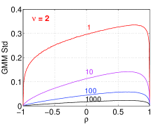
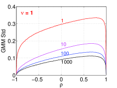
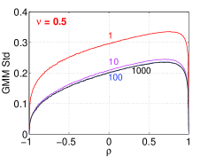
2 Simulations Based on t 𝑡 t
The bivariate t 𝑡 t t Σ , ν subscript 𝑡 Σ 𝜈
t_{\Sigma,\nu} t 𝑡 t Σ Σ \Sigma ν 𝜈 \nu Z ∼ N ( 0 , Σ ) similar-to 𝑍 𝑁 0 Σ Z\sim N(0,\Sigma) u ∼ χ ν 2 similar-to 𝑢 subscript superscript 𝜒 2 𝜈 u\sim\chi^{2}_{\nu} Z ν / u ∼ t Σ , ν similar-to 𝑍 𝜈 𝑢 subscript 𝑡 Σ 𝜈
Z\sqrt{\nu/u}\sim t_{\Sigma,\nu} Σ = [ 1 ρ ρ 1 ] Σ delimited-[] 1 𝜌 𝜌 1 \Sigma=\left[\begin{array}[]{cc}1&\rho\\
\rho&1\end{array}\right] − 1 ≤ ρ ≤ 1 1 𝜌 1 -1\leq\rho\leq 1 n 𝑛 n ( x i , y i ) ∼ t Σ , ν similar-to subscript 𝑥 𝑖 subscript 𝑦 𝑖 subscript 𝑡 Σ 𝜈
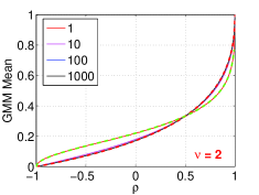
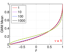
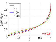
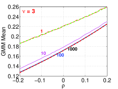
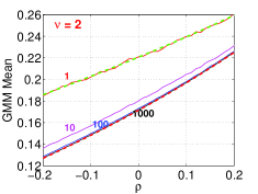
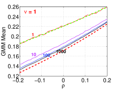
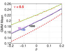
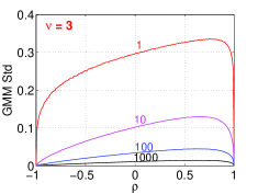
(x_{i},y_{i})\sim t_{\Sigma,\nu} G M M ( x , y ) = g n ( x , y ) 𝐺 𝑀 𝑀 𝑥 𝑦 subscript 𝑔 𝑛 𝑥 𝑦 GMM(x,y)=g_{n}(x,y) 7 n ∈ { 1 , 10 , 100 , 1000 , 10000 } 𝑛 1 10 100 1000 10000 n\in\{1,10,100,1000,10000\} ν ∈ { 3 , 2 , 1 , 0.5 } 𝜈 3 2 1 0.5 \nu\in\{3,2,1,0.5\} 1
The panels in the first (top) row present the mean of GMM (g n subscript 𝑔 𝑛 g_{n} f 1 subscript 𝑓 1 f_{1} f ∞ subscript 𝑓 f_{\infty}
f 1 = subscript 𝑓 1 absent \displaystyle f_{1}= ρ + 1 π [ 1 − ρ 2 log ( 2 − 2 ρ ) − 2 ρ sin − 1 ( ( 1 − ρ ) / 2 ) ] , f ∞ = 1 − ( 1 − ρ ) / 2 1 + ( 1 − ρ ) / 2 𝜌 1 𝜋 delimited-[] 1 superscript 𝜌 2 2 2 𝜌 2 𝜌 superscript 1 1 𝜌 2 subscript 𝑓
1 1 𝜌 2 1 1 𝜌 2 \displaystyle\rho+\frac{1}{\pi}\left[\sqrt{1-\rho^{2}}\log(2-2\rho)-2\rho\sin^{-1}\big{(}\sqrt{(1-\rho)/2}\big{)}\right],\hskip 10.84006ptf_{\infty}=\frac{1-\sqrt{(1-\rho)/2}}{1+\sqrt{(1-\rho)/2}} (8)
For better clarity, the panels in the second (middle) row plot the magnified portion. In each panel, the top (dashed and green if color is available) curve represent f 1 subscript 𝑓 1 f_{1} f ∞ subscript 𝑓 f_{\infty} ν = 3 𝜈 3 \nu=3 ν = 2 𝜈 2 \nu=2 g n subscript 𝑔 𝑛 g_{n} f ∞ subscript 𝑓 f_{\infty} ν = 1 𝜈 1 \nu=1 g n subscript 𝑔 𝑛 g_{n} f ∞ subscript 𝑓 f_{\infty} ν = 0.5 𝜈 0.5 \nu=0.5 g n subscript 𝑔 𝑛 g_{n} f ∞ subscript 𝑓 f_{\infty}
The panels in the third (bottom) row plot the standard deviation (std). For ν ≥ 1 𝜈 1 \nu\geq 1 ν = 1 𝜈 1 \nu=1 ν = 0.5 𝜈 0.5 \nu=0.5
Figure 1: We simulate G M M = g n 𝐺 𝑀 𝑀 subscript 𝑔 𝑛 GMM=g_{n} 7 t 𝑡 t ν = 0.5 , 1 , 2 , 3 𝜈 0.5 1 2 3
\nu=0.5,1,2,3 n = 1 , 10 , 100 , 1000 𝑛 1 10 100 1000
n=1,10,100,1000 f 1 subscript 𝑓 1 f_{1} f ∞ subscript 𝑓 f_{\infty} 8 g n subscript 𝑔 𝑛 g_{n}
Basically, the simulations suggest that g n subscript 𝑔 𝑛 g_{n} f ∞ subscript 𝑓 f_{\infty} ν > 1 𝜈 1 \nu>1 ν = 1 𝜈 1 \nu=1 g n subscript 𝑔 𝑛 g_{n}
Because ρ 𝜌 \rho g n → f ∞ → subscript 𝑔 𝑛 subscript 𝑓 g_{n}\rightarrow f_{\infty} ν ≥ 1 𝜈 1 \nu\geq 1 ρ 𝜌 \rho [14 ] , most natural datasets have the equivalent ν > 1 𝜈 1 \nu>1
3 Analysis Based on Elliptical Distributions
We consider ( x i , y i ) subscript 𝑥 𝑖 subscript 𝑦 𝑖 (x_{i},y_{i}) i = 1 𝑖 1 i=1 n 𝑛 n ( X , Y ) 𝑋 𝑌 (X,Y) n → ∞ → 𝑛 n\rightarrow\infty
G M M ( x , y ) = g n ( x , y ) = ∑ i = 1 n [ min ( x i + , y i + ) + min ( x i − , y i − ) ] ∑ i = 1 n [ max ( x i + , y i + ) + max ( x i − , y i − ) ] 𝐺 𝑀 𝑀 𝑥 𝑦 subscript 𝑔 𝑛 𝑥 𝑦 superscript subscript 𝑖 1 𝑛 delimited-[] subscript 𝑥 limit-from 𝑖 subscript 𝑦 limit-from 𝑖 subscript 𝑥 limit-from 𝑖 subscript 𝑦 limit-from 𝑖 superscript subscript 𝑖 1 𝑛 delimited-[] subscript 𝑥 limit-from 𝑖 subscript 𝑦 limit-from 𝑖 subscript 𝑥 limit-from 𝑖 subscript 𝑦 limit-from 𝑖 \displaystyle GMM(x,y)=g_{n}(x,y)=\frac{\sum_{i=1}^{n}\left[\min(x_{i+},y_{i+})+\min(x_{i-},y_{i-})\right]}{\sum_{i=1}^{n}\left[\max(x_{i+},y_{i+})+\max(x_{i-},y_{i-})\right]}
To proceed with the theoretical analysis, we make a very general distributional assumption on the data. We say the vector ( X , Y ) 𝑋 𝑌 (X,Y)
( X , Y ) T = A U T = ( a 1 T U T a 2 T U T ) superscript 𝑋 𝑌 𝑇 𝐴 𝑈 𝑇 binomial superscript subscript 𝑎 1 𝑇 𝑈 𝑇 superscript subscript 𝑎 2 𝑇 𝑈 𝑇 \displaystyle(X,Y)^{T}=AUT={a_{1}^{T}UT\choose a_{2}^{T}UT} (9)
where A = ( a 1 , a 2 ) T 𝐴 superscript subscript 𝑎 1 subscript 𝑎 2 𝑇 A=(a_{1},a_{2})^{T} 2 × 2 2 2 2\times 2 U 𝑈 U T 𝑇 T U 𝑈 U [1 ] for an introduction.
In the family of elliptical distributions, there are two important special cases:
1.
Gaussian distribution : In this case, we have T 2 ∼ χ 2 2 similar-to superscript 𝑇 2 subscript superscript 𝜒 2 2 T^{2}\sim\chi^{2}_{2}
( X , Y ) T ∼ N ( 0 , Σ ) ∼ A U χ 2 2 , where Σ = A A T = ( 1 σ ρ σ ρ σ 2 ) . formulae-sequence similar-to superscript 𝑋 𝑌 𝑇 𝑁 0 Σ similar-to 𝐴 𝑈 subscript superscript 𝜒 2 2 where Σ 𝐴 superscript 𝐴 𝑇 matrix 1 𝜎 𝜌 𝜎 𝜌 superscript 𝜎 2 \displaystyle(X,Y)^{T}\sim N(0,\Sigma)\sim AU\sqrt{\chi^{2}_{2}},\hskip 21.68121pt\text{where }\ \Sigma=AA^{T}=\begin{pmatrix}1&\sigma\rho\cr\sigma\rho&\sigma^{2}\end{pmatrix}. (10)
Note that for analyzing g n subscript 𝑔 𝑛 g_{n} Var ( X ) = 1 Var 𝑋 1 \hbox{\rm Var}(X)=1
2.
t 𝑡 t -distribution : In this case, we have T ∼ χ 2 2 ν / χ ν 2 similar-to 𝑇 subscript superscript 𝜒 2 2 𝜈 subscript superscript 𝜒 2 𝜈 T\sim\sqrt{\chi^{2}_{2}\nu/\chi^{2}_{\nu}}
( X , Y ) T ∼ N ( 0 , Σ ) ν / χ ν 2 . similar-to superscript 𝑋 𝑌 𝑇 𝑁 0 Σ 𝜈 subscript superscript 𝜒 2 𝜈 \displaystyle(X,Y)^{T}\sim N(0,\Sigma)\sqrt{\nu/\chi^{2}_{\nu}}. (11)
Note that in Σ Σ \Sigma σ ≠ 1 𝜎 1 \sigma\neq 1
•
Σ = ( 1 σ ρ σ ρ σ 2 ) Σ matrix 1 𝜎 𝜌 𝜎 𝜌 superscript 𝜎 2 \Sigma=\begin{pmatrix}1&\sigma\rho\cr\sigma\rho&\sigma^{2}\end{pmatrix} ρ ∈ [ − 1 , 1 ] 𝜌 1 1 \rho\in[-1,1] σ > 0 𝜎 0 \sigma>0
•
α = sin − 1 ( 1 / 2 − ρ / 2 ) ∈ [ 0 , π / 2 ] 𝛼 superscript 1 1 2 𝜌 2 0 𝜋 2 \alpha=\sin^{-1}\big{(}\sqrt{1/2-\rho/2}\big{)}\in[0,\pi/2]
•
τ ∈ [ − π / 2 + 2 α , π / 2 ] 𝜏 𝜋 2 2 𝛼 𝜋 2 \tau\in[-\pi/2+2\alpha,\pi/2] cos ( τ − 2 α ) / cos τ = σ 𝜏 2 𝛼 𝜏 𝜎 \cos(\tau-2\alpha)/\cos\tau=\sigma τ = arctan ( σ / sin ( 2 α ) − cot ( 2 α ) ) 𝜏 𝜎 2 𝛼 2 𝛼 \tau=\arctan(\sigma/\sin(2\alpha)-\cot(2\alpha)) τ = α 𝜏 𝛼 \tau=\alpha σ = 1 𝜎 1 \sigma=1
In addition, we need the following definitions of f 1 ( ρ , σ ) subscript 𝑓 1 𝜌 𝜎 f_{1}(\rho,\sigma) f ∞ ( ρ , σ ) subscript 𝑓 𝜌 𝜎 f_{\infty}(\rho,\sigma) σ 𝜎 \sigma σ = 1 𝜎 1 \sigma=1
f 1 ( ρ , σ ) = subscript 𝑓 1 𝜌 𝜎 absent \displaystyle f_{1}(\rho,\sigma)= 1 σ π ( ( τ + π / 2 − 2 α ) cos ( 2 α ) + sin ( 2 α ) log cos ( 2 α − π / 2 ) cos τ ) 1 𝜎 𝜋 𝜏 𝜋 2 2 𝛼 2 𝛼 2 𝛼 2 𝛼 𝜋 2 𝜏 \displaystyle\frac{1}{\sigma\pi}\Big{(}(\tau+\pi/2-2\alpha)\cos(2\alpha)+\sin(2\alpha)\log\frac{\cos(2\alpha-\pi/2)}{\cos\tau}\Big{)}
+ σ π ( ( π / 2 − τ ) cos ( 2 α ) + sin ( 2 α ) log cos ( 2 α − π / 2 ) cos ( 2 α − τ ) ) , 𝜎 𝜋 𝜋 2 𝜏 2 𝛼 2 𝛼 2 𝛼 𝜋 2 2 𝛼 𝜏 \displaystyle+\frac{\sigma}{\pi}\Big{(}(\pi/2-\tau)\cos(2\alpha)+\sin(2\alpha)\log\frac{\cos(2\alpha-\pi/2)}{\cos(2\alpha-\tau)}\Big{)}, (12)
= σ = 1 𝜎 1 \displaystyle\overset{\sigma=1}{=} ρ + 1 π [ 1 − ρ 2 log ( 2 − 2 ρ ) − 2 ρ sin − 1 ( ( 1 − ρ ) / 2 ) ] 𝜌 1 𝜋 delimited-[] 1 superscript 𝜌 2 2 2 𝜌 2 𝜌 superscript 1 1 𝜌 2 \displaystyle\rho+\frac{1}{\pi}\left[\sqrt{1-\rho^{2}}\log(2-2\rho)-2\rho\sin^{-1}\big{(}\sqrt{(1-\rho)/2}\big{)}\right] (13)
f ∞ ( ρ , σ ) = subscript 𝑓 𝜌 𝜎 absent \displaystyle f_{\infty}(\rho,\sigma)= 1 − sin ( 2 α − τ ) + σ ( 1 − sin τ ) σ ( 1 + sin τ ) + 1 + sin ( 2 α − τ ) 1 2 𝛼 𝜏 𝜎 1 𝜏 𝜎 1 𝜏 1 2 𝛼 𝜏 \displaystyle\frac{1-\sin(2\alpha-\tau)+\sigma(1-\sin\tau)}{\sigma(1+\sin\tau)+1+\sin(2\alpha-\tau)} (14)
= σ = 1 𝜎 1 \displaystyle\overset{\sigma=1}{=} 1 − ( 1 − ρ ) / 2 1 + ( 1 − ρ ) / 2 1 1 𝜌 2 1 1 𝜌 2 \displaystyle\frac{1-\sqrt{(1-\rho)/2}}{1+\sqrt{(1-\rho)/2}} (15)
Theorem 1
Theorem 1 .
(Consistency)
Assume ( X , Y ) X Y (X,Y) ( X , Y ) T = A U T superscript X Y T A U T (X,Y)^{T}=AUT Σ = A A T = ( 1 σ ρ σ ρ σ 2 ) Σ A superscript A T matrix 1 σ ρ σ ρ superscript σ 2 \Sigma=AA^{T}=\begin{pmatrix}1&\sigma\rho\cr\sigma\rho&\sigma^{2}\end{pmatrix} ( x i , y i ) subscript x i subscript y i (x_{i},y_{i}) i = 1 i 1 i=1 n n n ( X , Y ) X Y (X,Y) G M M ( x , y ) = g n ( x , y ) G M M x y subscript g n x y GMM(x,y)=g_{n}(x,y) 7
•
g 1 = f 1 ( ρ , σ ) subscript 𝑔 1 subscript 𝑓 1 𝜌 𝜎 g_{1}=f_{1}(\rho,\sigma)
•
If 𝔼 T < ∞ 𝔼 𝑇 {\mathbb{E}}T<\infty , then g n → f ∞ ( ρ , σ ) → subscript 𝑔 𝑛 subscript 𝑓 𝜌 𝜎 g_{n}\rightarrow f_{\infty}(\rho,\sigma) , almost surely.
•
If we have
lim t → ∞ t ℙ ( T > t ) 𝔼 min ( T , t ) = 0 , subscript → 𝑡 𝑡 ℙ 𝑇 𝑡 𝔼 𝑇 𝑡 0 \displaystyle\lim_{t\to\infty}\frac{t\,{\mathbb{P}}(T>t)}{{\mathbb{E}}\min(T,t)}=0, (16)
then g n → f ∞ ( ρ , σ ) → subscript 𝑔 𝑛 subscript 𝑓 𝜌 𝜎 g_{n}\rightarrow f_{\infty}(\rho,\sigma) , in probability.
•
If ( X , Y ) 𝑋 𝑌 (X,Y) has a t 𝑡 t -distribution with ν 𝜈 \nu degrees of freedom, then g n → f ∞ ( ρ , σ ) → subscript 𝑔 𝑛 subscript 𝑓 𝜌 𝜎 g_{n}\rightarrow f_{\infty}(\rho,\sigma) almost surely if ν > 1 𝜈 1 \nu>1 and g n → f ∞ ( ρ , σ ) → subscript 𝑔 𝑛 subscript 𝑓 𝜌 𝜎 g_{n}\rightarrow f_{\infty}(\rho,\sigma) in probability if ν = 1 𝜈 1 \nu=1 .
Theorem 2
Theorem 2 .
(Asymptotic Normality)
1
•
If 𝔼 T 2 < ∞ 𝔼 superscript 𝑇 2 {\mathbb{E}}T^{2}<\infty , then
n 1 / 2 ( g n ( x , y ) − f ∞ ( ρ , σ ) ) ⟶ 𝐷 N ( 0 , V H 4 𝔼 T 2 𝔼 2 T ) superscript 𝑛 1 2 subscript 𝑔 𝑛 𝑥 𝑦 subscript 𝑓 𝜌 𝜎 𝐷 ⟶ 𝑁 0 𝑉 superscript 𝐻 4 𝔼 superscript 𝑇 2 superscript 𝔼 2 𝑇 \displaystyle n^{1/2}\left(g_{n}(x,y)-f_{\infty}(\rho,\sigma)\right)\overset{D}{\longrightarrow}N\left(0,\frac{V}{H^{4}}\frac{{\mathbb{E}}T^{2}}{{\mathbb{E}}^{2}T}\right) (17)
where
V 𝑉 \displaystyle V (18)
= \displaystyle= 1 4 π 3 { 2 τ + π − 4 α + sin ( 2 τ − 4 α ) + σ 2 ( π − 2 τ − sin ( 2 τ ) ) } { σ ( 1 + sin τ ) + 1 + sin ( 2 α − τ ) } 2 1 4 superscript 𝜋 3 2 𝜏 𝜋 4 𝛼 2 𝜏 4 𝛼 superscript 𝜎 2 𝜋 2 𝜏 2 𝜏 superscript 𝜎 1 𝜏 1 2 𝛼 𝜏 2 \displaystyle\frac{1}{4\pi^{3}}\left\{2\tau+\pi-4\alpha+\sin(2\tau-4\alpha)+\sigma^{2}\left(\pi-2\tau-\sin(2\tau)\right)\right\}\left\{\sigma(1+\sin\tau)+1+\sin(2\alpha-\tau)\right\}^{2}
+ \displaystyle+ 1 4 π 3 { σ 2 ( 2 τ + sin ( 2 τ ) + π ) + ( π + 4 α − 2 τ − sin ( 2 τ − 4 α ) ) + 4 σ ( sin 2 α − 2 α cos 2 α ) } 1 4 superscript 𝜋 3 superscript 𝜎 2 2 𝜏 2 𝜏 𝜋 𝜋 4 𝛼 2 𝜏 2 𝜏 4 𝛼 4 𝜎 2 𝛼 2 𝛼 2 𝛼 \displaystyle\frac{1}{4\pi^{3}}\left\{\sigma^{2}\left(2{\tau}+\sin(2\tau)+{\pi}\right)+\left({\pi}+4\alpha-2{\tau}-\sin(2\tau-4\alpha)\right)+4{\sigma}\left(\sin 2\alpha-2\alpha\cos 2\alpha\right)\right\}
× { 1 − sin ( 2 α − τ ) + σ ( 1 − sin τ ) } 2 absent superscript 1 2 𝛼 𝜏 𝜎 1 𝜏 2 \displaystyle\hskip 14.45377pt\times\left\{1-\sin(2\alpha-\tau)+\sigma(1-\sin\tau)\right\}^{2}
− \displaystyle- σ π 3 ( ( π − 2 α ) cos 2 α + sin 2 α ) { 1 − sin ( 2 α − τ ) + σ ( 1 − sin τ ) } { σ ( 1 + sin τ ) + 1 + sin ( 2 α − τ ) } 𝜎 superscript 𝜋 3 𝜋 2 𝛼 2 𝛼 2 𝛼 1 2 𝛼 𝜏 𝜎 1 𝜏 𝜎 1 𝜏 1 2 𝛼 𝜏 \displaystyle\frac{\sigma}{\pi^{3}}\left((\pi-2\alpha)\cos 2\alpha+\sin 2\alpha\right)\left\{1-\sin(2\alpha-\tau)+\sigma(1-\sin\tau)\right\}\left\{\sigma(1+\sin\tau)+1+\sin(2\alpha-\tau)\right\}
= σ = 1 𝜎 1 \displaystyle\overset{\sigma=1}{=} 4 π 3 sin 2 α ( 3 π − 8 cos α + 2 sin 2 α + π cos 2 α − 8 α sin α − 4 α cos 2 α ) 4 superscript 𝜋 3 superscript 2 𝛼 3 𝜋 8 𝛼 2 2 𝛼 𝜋 2 𝛼 8 𝛼 𝛼 4 𝛼 2 𝛼 \displaystyle\frac{4}{\pi^{3}}\sin^{2}\alpha\left(3\pi-8\cos\alpha+2\sin 2\alpha+\pi\cos 2\alpha-8\alpha\sin\alpha-4\alpha\cos 2\alpha\right) (19)
and
H = 𝐻 absent \displaystyle H= 1 π { σ ( 1 + sin τ ) + 1 + sin ( 2 α − τ ) } = σ = 1 2 π ( 1 + sin α ) 1 𝜋 𝜎 1 𝜏 1 2 𝛼 𝜏 𝜎 1 2 𝜋 1 𝛼 \displaystyle\frac{1}{\pi}\left\{\sigma(1+\sin\tau)+1+\sin(2\alpha-\tau)\right\}\overset{\sigma=1}{=}\frac{2}{\pi}(1+\sin\alpha) (20)
•
If ( X , Y ) 𝑋 𝑌 (X,Y) has a t 𝑡 t -distribution with ν 𝜈 \nu degrees of freedom and ν > 2 𝜈 2 \nu>2 , then
n 1 / 2 ( g n ( x , y ) − f ∞ ( ρ , σ ) ) ⟶ D N ( 0 , V H 4 𝔼 T 2 𝔼 2 T ) . superscript ⟶ D superscript 𝑛 1 2 subscript 𝑔 𝑛 𝑥 𝑦 subscript 𝑓 𝜌 𝜎 𝑁 0 𝑉 superscript 𝐻 4 𝔼 superscript 𝑇 2 superscript 𝔼 2 𝑇 \displaystyle n^{1/2}\left(g_{n}(x,y)-f_{\infty}(\rho,\sigma)\right)\stackrel{{\scriptstyle{\rm D}}}{{\longrightarrow}}N\left(0,\frac{V}{H^{4}}\frac{{\mathbb{E}}T^{2}}{{\mathbb{E}}^{2}T}\right). (21)
where 𝔼 T 2 = 2 ν ν − 2 𝔼 superscript 𝑇 2 2 𝜈 𝜈 2 {\mathbb{E}}T^{2}=\frac{2\nu}{\nu-2} and 𝔼 T = ν Γ ( ν / 2 − 1 / 2 ) Γ ( 1 / 2 ) 2 Γ ( ν / 2 ) 𝔼 𝑇 𝜈 Γ 𝜈 2 1 2 Γ 1 2 2 Γ 𝜈 2 {\mathbb{E}}T=\frac{\sqrt{\nu}\,\Gamma(\nu/2-1/2)\Gamma(1/2)}{2\,\Gamma(\nu/2)}
•
If ( X , Y ) 𝑋 𝑌 (X,Y) has a t 𝑡 t -distribution with ν = 2 𝜈 2 \nu=2 degrees of freedom, then
( n log n ) 1 / 2 ( g n ( x , y ) − f ∞ ( ρ , σ ) ) ⟶ D N ( 0 , V H 4 4 π 2 ) . superscript ⟶ D superscript 𝑛 𝑛 1 2 subscript 𝑔 𝑛 𝑥 𝑦 subscript 𝑓 𝜌 𝜎 𝑁 0 𝑉 superscript 𝐻 4 4 superscript 𝜋 2 \displaystyle\left(\frac{n}{\log n}\right)^{1/2}\left(g_{n}(x,y)-f_{\infty}(\rho,\sigma)\right)\stackrel{{\scriptstyle{\rm D}}}{{\longrightarrow}}N\left(0,\frac{V}{H^{4}}\frac{4}{\pi^{2}}\right). (22)
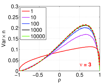
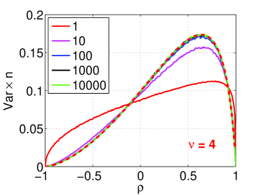
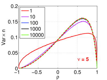
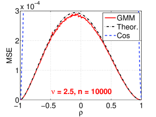
Figure 2
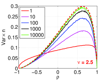
V a r ( g n ) = 1 n V H 4 𝔼 T 2 𝔼 2 T + O ( 1 n 2 ) 𝑉 𝑎 𝑟 subscript 𝑔 𝑛 1 𝑛 𝑉 superscript 𝐻 4 𝔼 superscript 𝑇 2 superscript 𝔼 2 𝑇 𝑂 1 superscript 𝑛 2 \displaystyle Var\left(g_{n}\right)=\frac{1}{n}\frac{V}{H^{4}}\frac{{\mathbb{E}}T^{2}}{{\mathbb{E}}^{2}T}+O\left(\frac{1}{n^{2}}\right) (23)
by considering that the data follow a t 𝑡 t ν 𝜈 \nu ν = 2.5 , 3 , 4 , 5 𝜈 2.5 3 4 5
\nu=2.5,\ 3,\ 4,\ 5 n 𝑛 n n 𝑛 n 23
Figure 2: Simulations for verifying the asymptotic variance formula (23 t 𝑡 t ν 𝜈 \nu ν ∈ { 2.5 , 3 , 4 , 5 } 𝜈 2.5 3 4 5 \nu\in\{2.5,3,4,5\} ρ ∈ [ − 1 , 1 ] 𝜌 1 1 \rho\in[-1,1] V a r ( g n ) × n 𝑉 𝑎 𝑟 subscript 𝑔 𝑛 𝑛 Var(g_{n})\times n V H 4 𝔼 T 2 𝔼 2 T 𝑉 superscript 𝐻 4 𝔼 superscript 𝑇 2 superscript 𝔼 2 𝑇 \frac{V}{H^{4}}\frac{{\mathbb{E}}T^{2}}{{\mathbb{E}}^{2}T} n 𝑛 n 23 n 𝑛 n
4 Estimation of ρ 𝜌 \rho
The fact that g n ( x , y ) → f ∞ ( ρ , σ ) → subscript 𝑔 𝑛 𝑥 𝑦 subscript 𝑓 𝜌 𝜎 g_{n}(x,y)\rightarrow f_{\infty}(\rho,\sigma) σ = 1 𝜎 1 \sigma=1 f ∞ = 1 − ( 1 − ρ ) / 2 1 + ( 1 − ρ ) / 2 subscript 𝑓 1 1 𝜌 2 1 1 𝜌 2 f_{\infty}=\frac{1-\sqrt{(1-\rho)/2}}{1+\sqrt{(1-\rho)/2}} ρ 𝜌 \rho
ρ ^ g = 1 − 2 ( 1 − g n 1 + g n ) 2 subscript ^ 𝜌 𝑔 1 2 superscript 1 subscript 𝑔 𝑛 1 subscript 𝑔 𝑛 2 \displaystyle\hat{\rho}_{g}=1-2\left(\frac{1-g_{n}}{1+g_{n}}\right)^{2} (24)
As n → ∞ → 𝑛 n\rightarrow\infty g n → f ∞ → subscript 𝑔 𝑛 subscript 𝑓 g_{n}\rightarrow f_{\infty} ρ ^ g → ρ → subscript ^ 𝜌 𝑔 𝜌 \hat{\rho}_{g}\rightarrow\rho ρ ^ g subscript ^ 𝜌 𝑔 \hat{\rho}_{g} ρ ^ g subscript ^ 𝜌 𝑔 \hat{\rho}_{g}
V a r ( ρ ^ g ) = 𝑉 𝑎 𝑟 subscript ^ 𝜌 𝑔 absent \displaystyle Var\left(\hat{\rho}_{g}\right)= [ 8 1 − f ∞ ( 1 + f ∞ ) 3 ] 2 V a r ( g n ) + O ( 1 n 2 ) superscript delimited-[] 8 1 subscript 𝑓 superscript 1 subscript 𝑓 3 2 𝑉 𝑎 𝑟 subscript 𝑔 𝑛 𝑂 1 superscript 𝑛 2 \displaystyle\left[8\frac{1-f_{\infty}}{(1+f_{\infty})^{3}}\right]^{2}Var\left(g_{n}\right)+O\left(\frac{1}{n^{2}}\right)
= \displaystyle= 1 n 2 ( 1 − ρ ) ( 1 + ( 1 − ρ ) / 2 ) 4 V H 4 𝔼 T 2 𝔼 2 T + O ( 1 n 2 ) 1 𝑛 2 1 𝜌 superscript 1 1 𝜌 2 4 𝑉 superscript 𝐻 4 𝔼 superscript 𝑇 2 superscript 𝔼 2 𝑇 𝑂 1 superscript 𝑛 2 \displaystyle\frac{1}{n}2\left(1-\rho\right)\left(1+\sqrt{(1-\rho)/2}\right)^{4}\frac{V}{H^{4}}\frac{{\mathbb{E}}T^{2}}{{\mathbb{E}}^{2}T}+O\left(\frac{1}{n^{2}}\right) (25)
See (23 2 ρ ^ g subscript ^ 𝜌 𝑔 \hat{\rho}_{g} 𝔼 T < ∞ 𝔼 𝑇 {\mathbb{E}}T<\infty V a r ( ρ ^ g ) < ∞ 𝑉 𝑎 𝑟 subscript ^ 𝜌 𝑔 Var\left(\hat{\rho}_{g}\right)<\infty 𝔼 T 2 < ∞ 𝔼 superscript 𝑇 2 {\mathbb{E}}T^{2}<\infty
It is interesting to compare this estimator with the commonly used estimator based on the “cosine” similarity:
C o s ( x , y ) = ∑ i = 1 n x i y i ∑ i = 1 n x i 2 ∑ i = 1 n y i 2 = △ c n ( x , y ) 𝐶 𝑜 𝑠 𝑥 𝑦 superscript subscript 𝑖 1 𝑛 subscript 𝑥 𝑖 subscript 𝑦 𝑖 superscript subscript 𝑖 1 𝑛 superscript subscript 𝑥 𝑖 2 superscript subscript 𝑖 1 𝑛 superscript subscript 𝑦 𝑖 2 △ subscript 𝑐 𝑛 𝑥 𝑦 \displaystyle Cos(x,y)=\frac{\sum_{i=1}^{n}x_{i}y_{i}}{\sqrt{\sum_{i=1}^{n}x_{i}^{2}\sum_{i=1}^{n}y_{i}^{2}}}\overset{\triangle}{=}c_{n}(x,y)
When the data are bivariate normal, it is a known result [1 ] that c n ( x , y ) subscript 𝑐 𝑛 𝑥 𝑦 c_{n}(x,y)
n 1 / 2 ( c n − ρ ) ⟶ 𝐷 N ( 0 , ( 1 − ρ 2 ) 2 ) superscript 𝑛 1 2 subscript 𝑐 𝑛 𝜌 𝐷 ⟶ 𝑁 0 superscript 1 superscript 𝜌 2 2 \displaystyle n^{1/2}\left(c_{n}-\rho\right)\overset{D}{\longrightarrow}N\left(0,(1-\rho^{2})^{2}\right) (26)
This asymptotic normality (with difference in the variance term) holds as long as the data have bounded fourth moment. Here, we present the generalization as a theorem.
Theorem 3 .
If 𝔼 T 4 < ∞ 𝔼 superscript 𝑇 4 {\mathbb{E}}T^{4}<\infty
n 1 / 2 ( c n − ρ ) ⟶ 𝐷 N ( 0 , 𝔼 T 4 2 𝔼 2 T 2 ( 1 − ρ 2 ) 2 ) superscript 𝑛 1 2 subscript 𝑐 𝑛 𝜌 𝐷 ⟶ 𝑁 0 𝔼 superscript 𝑇 4 2 superscript 𝔼 2 superscript 𝑇 2 superscript 1 superscript 𝜌 2 2 \displaystyle n^{1/2}\left(c_{n}-\rho\right)\overset{D}{\longrightarrow}N\left(0,\frac{{\mathbb{E}}T^{4}}{2{\mathbb{E}}^{2}T^{2}}(1-\rho^{2})^{2}\right) (27)
Based on Theorem 3 ρ 𝜌 \rho
ρ ^ c = c n , V a r ( ρ ^ c ) = 1 n 𝔼 T 4 2 𝔼 2 T 2 ( 1 − ρ 2 ) 2 + O ( 1 n 2 ) formulae-sequence subscript ^ 𝜌 𝑐 subscript 𝑐 𝑛 𝑉 𝑎 𝑟 subscript ^ 𝜌 𝑐 1 𝑛 𝔼 superscript 𝑇 4 2 superscript 𝔼 2 superscript 𝑇 2 superscript 1 superscript 𝜌 2 2 𝑂 1 superscript 𝑛 2 \displaystyle\hat{\rho}_{c}=c_{n},\hskip 14.45377ptVar\left(\hat{\rho}_{c}\right)=\frac{1}{n}\frac{{\mathbb{E}}T^{4}}{2{\mathbb{E}}^{2}T^{2}}\left(1-\rho^{2}\right)^{2}+O\left(\frac{1}{n^{2}}\right) (28)
When the data follow a t 𝑡 t ν 𝜈 \nu
𝔼 T 2 = 2 ν ν − 2 , 𝔼 T 4 = 4 ν 3 ( ν − 2 ) 2 ( ν − 4 ) + 4 ν 2 ( ν − 2 ) 2 formulae-sequence 𝔼 superscript 𝑇 2 2 𝜈 𝜈 2 𝔼 superscript 𝑇 4 4 superscript 𝜈 3 superscript 𝜈 2 2 𝜈 4 4 superscript 𝜈 2 superscript 𝜈 2 2 \displaystyle{\mathbb{E}}T^{2}=\frac{2\nu}{\nu-2},\hskip 21.68121pt{\mathbb{E}}T^{4}=\frac{4\nu^{3}}{(\nu-2)^{2}(\nu-4)}+\frac{4\nu^{2}}{(\nu-2)^{2}}
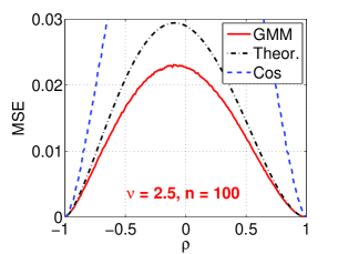
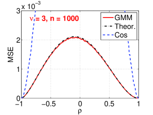
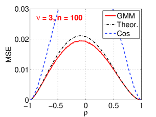
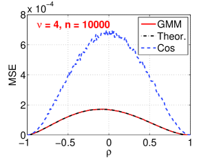
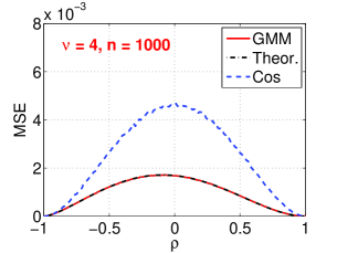
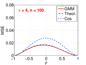
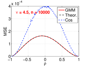
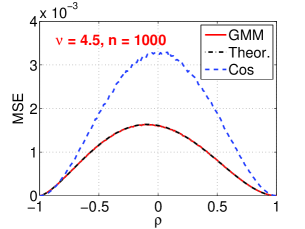
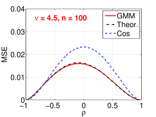
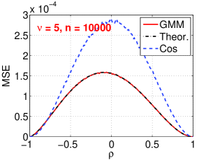
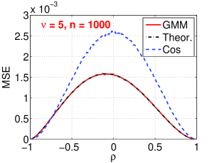
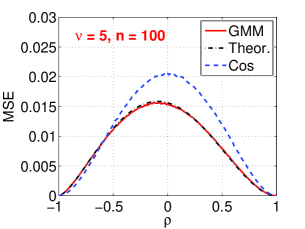
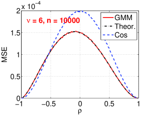
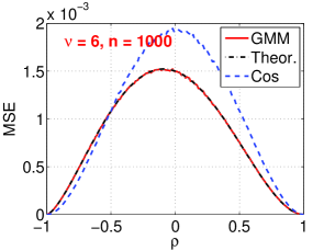
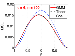
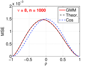
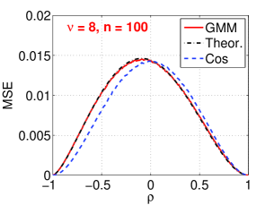
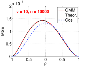
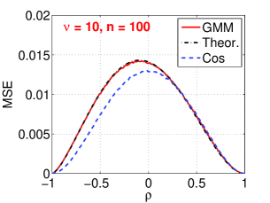
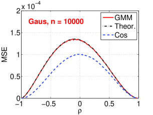
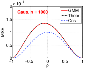
Figure 3 4 ρ ^ g subscript ^ 𝜌 𝑔 \hat{\rho}_{g} ρ ^ c subscript ^ 𝜌 𝑐 \hat{\rho}_{c} t 𝑡 t ν 𝜈 \nu ν ∈ { 2.5 , 3 , 4 , 4.5 , 5 , 6 , 8 , 10 } 𝜈 2.5 3 4 4.5 5 6 8 10 \nu\in\{2.5,3,4,4.5,5,6,8,10\} ν = ∞ 𝜈 \nu=\infty M S E ( ρ ^ g ) 𝑀 𝑆 𝐸 subscript ^ 𝜌 𝑔 MSE(\hat{\rho}_{g}) M S E ( ρ ^ c ) 𝑀 𝑆 𝐸 subscript ^ 𝜌 𝑐 MSE(\hat{\rho}_{c}) ρ ^ g subscript ^ 𝜌 𝑔 \hat{\rho}_{g} 1 n 2 ( 1 − ρ ) ( 1 + ( 1 − ρ ) / 2 ) 4 V H 4 𝔼 T 2 𝔼 2 T 1 𝑛 2 1 𝜌 superscript 1 1 𝜌 2 4 𝑉 superscript 𝐻 4 𝔼 superscript 𝑇 2 superscript 𝔼 2 𝑇 \frac{1}{n}2\left(1-\rho\right)\left(1+\sqrt{(1-\rho)/2}\right)^{4}\frac{V}{H^{4}}\frac{{\mathbb{E}}T^{2}}{{\mathbb{E}}^{2}T} ρ ^ c subscript ^ 𝜌 𝑐 \hat{\rho}_{c}
The results in Figure 3 4 ρ ^ g subscript ^ 𝜌 𝑔 \hat{\rho}_{g} ρ ^ c subscript ^ 𝜌 𝑐 \hat{\rho}_{c} ν < 8 𝜈 8 \nu<8 ρ ^ g subscript ^ 𝜌 𝑔 \hat{\rho}_{g} 4 ρ ^ g subscript ^ 𝜌 𝑔 \hat{\rho}_{g} ρ ^ c subscript ^ 𝜌 𝑐 \hat{\rho}_{c}
Figure 3: Simulations for comparing two estimators of data similarity ρ 𝜌 \rho ρ ^ g subscript ^ 𝜌 𝑔 \hat{\rho}_{g} ρ ^ c subscript ^ 𝜌 𝑐 \hat{\rho}_{c} t 𝑡 t ν 𝜈 \nu ν 𝜈 \nu ρ ^ g subscript ^ 𝜌 𝑔 \hat{\rho}_{g} ρ ^ c subscript ^ 𝜌 𝑐 \hat{\rho}_{c} ρ ^ g subscript ^ 𝜌 𝑔 \hat{\rho}_{g} 1 n 2 ( 1 − ρ ) ( 1 + ( 1 − ρ ) / 2 ) 4 V H 4 𝔼 T 2 𝔼 2 T 1 𝑛 2 1 𝜌 superscript 1 1 𝜌 2 4 𝑉 superscript 𝐻 4 𝔼 superscript 𝑇 2 superscript 𝔼 2 𝑇 \frac{1}{n}2\left(1-\rho\right)\left(1+\sqrt{(1-\rho)/2}\right)^{4}\frac{V}{H^{4}}\frac{{\mathbb{E}}T^{2}}{{\mathbb{E}}^{2}T} ρ ^ g subscript ^ 𝜌 𝑔 \hat{\rho}_{g} ρ ^ c subscript ^ 𝜌 𝑐 \hat{\rho}_{c} ν 𝜈 \nu
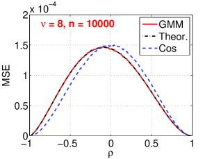
Figure 4: Continued from Figure 3 ν 𝜈 \nu ν = ∞ 𝜈 \nu=\infty ν < 8 𝜈 8 \nu<8 ρ ^ g subscript ^ 𝜌 𝑔 \hat{\rho}_{g} ρ ^ g subscript ^ 𝜌 𝑔 \hat{\rho}_{g}
Appendix A Proof of Theorem 1
For a random vector ( X , Y ) 𝑋 𝑌 (X,Y)
μ 1 = 𝔼 X + ∧ Y + + X − ∧ Y − X + ∨ Y + + X − ∨ Y − , μ ∞ = 𝔼 ( X + ∧ Y + + X − ∧ Y − ) 𝔼 ( X + ∨ Y + + X − ∨ Y − ) . formulae-sequence subscript 𝜇 1 𝔼 subscript 𝑋 subscript 𝑌 subscript 𝑋 subscript 𝑌 subscript 𝑋 subscript 𝑌 subscript 𝑋 subscript 𝑌 subscript 𝜇 𝔼 subscript 𝑋 subscript 𝑌 subscript 𝑋 subscript 𝑌 𝔼 subscript 𝑋 subscript 𝑌 subscript 𝑋 subscript 𝑌 \displaystyle\mu_{1}={\mathbb{E}}\,\frac{X_{+}\wedge Y_{+}+X_{-}\wedge Y_{-}}{X_{+}\vee Y_{+}+X_{-}\vee Y_{-}},\quad\mu_{\infty}=\frac{{\mathbb{E}}(X_{+}\wedge Y_{+}+X_{-}\wedge Y_{-})}{{\mathbb{E}}(X_{+}\vee Y_{+}+X_{-}\vee Y_{-})}.
Without any assumption, we have
μ 1 = 𝔼 X + ∧ Y + X + ∨ Y + + 𝔼 X − ∧ Y − X − ∨ Y − = 𝔼 | X | ∧ | Y | | X | ∨ | Y | I { X Y > 0 } = 𝔼 | X / Y | ∧ 1 | X / Y | ∨ 1 I { X / Y > 0 } . subscript 𝜇 1 𝔼 subscript 𝑋 subscript 𝑌 subscript 𝑋 subscript 𝑌 𝔼 subscript 𝑋 subscript 𝑌 subscript 𝑋 subscript 𝑌 𝔼 𝑋 𝑌 𝑋 𝑌 𝐼 𝑋 𝑌 0 𝔼 𝑋 𝑌 1 𝑋 𝑌 1 𝐼 𝑋 𝑌 0 \displaystyle\mu_{1}={\mathbb{E}}\,\frac{X_{+}\wedge Y_{+}}{X_{+}\vee Y_{+}}+{\mathbb{E}}\,\frac{X_{-}\wedge Y_{-}}{X_{-}\vee Y_{-}}={\mathbb{E}}\,\frac{|X|\wedge|Y|}{|X|\vee|Y|}I\{XY>0\}={\mathbb{E}}\,\frac{|X/Y|\wedge 1}{|X/Y|\vee 1}I\{X/Y>0\}.
When 𝔼 ( | X | ∧ | Y | ) < ∞ 𝔼 𝑋 𝑌 {\mathbb{E}}(|X|\wedge|Y|)<\infty
μ ∞ = 𝔼 ( | X | ∧ | Y | ) I { X Y > 0 } 𝔼 [ ( | X | + | Y | ) I { X Y ≤ 0 } + ( | X | ∨ | Y | ) I { X Y > 0 } ] . subscript 𝜇 𝔼 𝑋 𝑌 𝐼 𝑋 𝑌 0 𝔼 delimited-[] 𝑋 𝑌 𝐼 𝑋 𝑌 0 𝑋 𝑌 𝐼 𝑋 𝑌 0 \displaystyle\mu_{\infty}=\frac{{\mathbb{E}}(|X|\wedge|Y|)I\{XY>0\}}{{\mathbb{E}}\big{[}(|X|+|Y|)I\{XY\leq 0\}+(|X|\vee|Y|)I\{XY>0\}\big{]}}.
If ( X , Y ) 𝑋 𝑌 (X,Y) ( X , Y ) ∼ ( − X , − Y ) similar-to 𝑋 𝑌 𝑋 𝑌 (X,Y)\sim(-X,-Y)
μ 1 = 2 𝔼 X + ∧ Y + X + ∨ Y + subscript 𝜇 1 2 𝔼 subscript 𝑋 subscript 𝑌 subscript 𝑋 subscript 𝑌 \displaystyle\mu_{1}=2\,{\mathbb{E}}\,\frac{X_{+}\wedge Y_{+}}{X_{+}\vee Y_{+}}
and
μ ∞ = 𝔼 ( X + ∧ Y + ) 𝔼 ( X + ∨ Y + ) . subscript 𝜇 𝔼 subscript 𝑋 subscript 𝑌 𝔼 subscript 𝑋 subscript 𝑌 \displaystyle\mu_{\infty}=\frac{{\mathbb{E}}(X_{+}\wedge Y_{+})}{{\mathbb{E}}(X_{+}\vee Y_{+})}.
The vector ( X , Y ) 𝑋 𝑌 (X,Y)
( X , Y ) T = A U T = ( a 1 T U T a 2 T U T ) superscript 𝑋 𝑌 𝑇 𝐴 𝑈 𝑇 binomial superscript subscript 𝑎 1 𝑇 𝑈 𝑇 superscript subscript 𝑎 2 𝑇 𝑈 𝑇 \displaystyle(X,Y)^{T}=AUT={a_{1}^{T}UT\choose a_{2}^{T}UT}
where A = ( a 1 , a 2 ) T 𝐴 superscript subscript 𝑎 1 subscript 𝑎 2 𝑇 A=(a_{1},a_{2})^{T} 2 × 2 2 2 2\times 2 U 𝑈 U T 𝑇 T U 𝑈 U U ∼ − U similar-to 𝑈 𝑈 U\sim-U ( X , Y ) 𝑋 𝑌 (X,Y) T 𝑇 T T 𝑇 T μ 1 subscript 𝜇 1 \mu_{1} μ ∞ subscript 𝜇 \mu_{\infty}
μ 1 = 2 𝔼 ( a 1 T U ) + ∧ ( a 2 T U ) + ( a 1 T U ) + ∨ ( a 2 T U ) + subscript 𝜇 1 2 𝔼 subscript superscript subscript 𝑎 1 𝑇 𝑈 subscript superscript subscript 𝑎 2 𝑇 𝑈 subscript superscript subscript 𝑎 1 𝑇 𝑈 subscript superscript subscript 𝑎 2 𝑇 𝑈 \displaystyle\mu_{1}=2\,{\mathbb{E}}\,\frac{(a_{1}^{T}U)_{+}\wedge(a_{2}^{T}U)_{+}}{(a_{1}^{T}U)_{+}\vee(a_{2}^{T}U)_{+}}
and
μ ∞ = 𝔼 { ( a 1 T U ) + ∧ ( a 2 T U ) + } 𝔼 { ( a 1 T U ) + ∨ ( a 2 T U ) + } . subscript 𝜇 𝔼 subscript superscript subscript 𝑎 1 𝑇 𝑈 subscript superscript subscript 𝑎 2 𝑇 𝑈 𝔼 subscript superscript subscript 𝑎 1 𝑇 𝑈 subscript superscript subscript 𝑎 2 𝑇 𝑈 \displaystyle\mu_{\infty}=\frac{{\mathbb{E}}\{(a_{1}^{T}U)_{+}\wedge(a_{2}^{T}U)_{+}\}}{{\mathbb{E}}\{(a_{1}^{T}U)_{+}\vee(a_{2}^{T}U)_{+}\}}.
Since a bivariate Gaussian distribution is elliptical with T 2 ∼ χ 2 2 similar-to superscript 𝑇 2 subscript superscript 𝜒 2 2 T^{2}\sim\chi^{2}_{2} 𝔼 T 𝔼 𝑇 {\mathbb{E}}T
( X , Y ) ∼ N ( 0 , Σ ) with Σ = A A T = ( 1 σ ρ σ ρ σ 2 ) . similar-to 𝑋 𝑌 𝑁 0 Σ with Σ 𝐴 superscript 𝐴 𝑇 matrix 1 𝜎 𝜌 𝜎 𝜌 superscript 𝜎 2 \displaystyle(X,Y)\sim N(0,\Sigma)\ \hbox{ with }\ \Sigma=AA^{T}=\begin{pmatrix}1&\sigma\rho\cr\sigma\rho&\sigma^{2}\end{pmatrix}.
Note that we set Var ( X ) = 1 Var 𝑋 1 \hbox{\rm Var}(X)=1 μ 1 subscript 𝜇 1 \mu_{1} μ ∞ subscript 𝜇 \mu_{\infty}
For σ > 0 𝜎 0 \sigma>0 ρ ∈ [ − 1 , 1 ] 𝜌 1 1 \rho\in[-1,1] α = sin − 1 ( 1 / 2 − ρ / 2 ) ∈ [ 0 , π / 2 ] 𝛼 superscript 1 1 2 𝜌 2 0 𝜋 2 \alpha=\sin^{-1}\big{(}\sqrt{1/2-\rho/2}\big{)}\in[0,\pi/2] τ ∈ [ − π / 2 + 2 α , π / 2 ] 𝜏 𝜋 2 2 𝛼 𝜋 2 \tau\in[-\pi/2+2\alpha,\pi/2] cos ( τ − 2 α ) / cos τ = σ 𝜏 2 𝛼 𝜏 𝜎 \cos(\tau-2\alpha)/\cos\tau=\sigma τ = arctan ( σ / sin ( 2 α ) − cot ( 2 α ) ) 𝜏 𝜎 2 𝛼 2 𝛼 \tau=\arctan(\sigma/\sin(2\alpha)-\cot(2\alpha))
f 1 ( ρ , σ ) subscript 𝑓 1 𝜌 𝜎 \displaystyle f_{1}(\rho,\sigma) = \displaystyle= 1 σ π ( ( τ + π / 2 − 2 α ) cos ( 2 α ) + sin ( 2 α ) log cos ( 2 α − π / 2 ) cos τ ) 1 𝜎 𝜋 𝜏 𝜋 2 2 𝛼 2 𝛼 2 𝛼 2 𝛼 𝜋 2 𝜏 \displaystyle\frac{1}{\sigma\pi}\Big{(}(\tau+\pi/2-2\alpha)\cos(2\alpha)+\sin(2\alpha)\log\frac{\cos(2\alpha-\pi/2)}{\cos\tau}\Big{)}
+ σ π ( ( π / 2 − τ ) cos ( 2 α ) + sin ( 2 α ) log cos ( 2 α − π / 2 ) cos ( 2 α − τ ) ) , 𝜎 𝜋 𝜋 2 𝜏 2 𝛼 2 𝛼 2 𝛼 𝜋 2 2 𝛼 𝜏 \displaystyle+\frac{\sigma}{\pi}\Big{(}(\pi/2-\tau)\cos(2\alpha)+\sin(2\alpha)\log\frac{\cos(2\alpha-\pi/2)}{\cos(2\alpha-\tau)}\Big{)},
and
f ∞ ( ρ , σ ) = 1 − sin ( 2 α − τ ) + σ ( 1 − sin τ ) σ ( 1 + sin τ ) + 1 + sin ( 2 α − τ ) . subscript 𝑓 𝜌 𝜎 1 2 𝛼 𝜏 𝜎 1 𝜏 𝜎 1 𝜏 1 2 𝛼 𝜏 \displaystyle f_{\infty}(\rho,\sigma)=\frac{1-\sin(2\alpha-\tau)+\sigma(1-\sin\tau)}{\sigma(1+\sin\tau)+1+\sin(2\alpha-\tau)}.
We note that sin ( 2 α ) = 2 sin α cos α = 2 1 / 2 − ρ / 2 1 / 2 + ρ / 2 = 1 − ρ 2 2 𝛼 2 𝛼 𝛼 2 1 2 𝜌 2 1 2 𝜌 2 1 superscript 𝜌 2 \sin(2\alpha)=2\sin\alpha\cos\alpha=2\sqrt{1/2-\rho/2}\sqrt{1/2+\rho/2}=\sqrt{1-\rho^{2}} cos ( 2 α ) = ρ 2 𝛼 𝜌 \cos(2\alpha)=\rho cos ( 2 α − π / 2 ) = sin ( 2 α ) = 1 − ρ 2 2 𝛼 𝜋 2 2 𝛼 1 superscript 𝜌 2 \cos(2\alpha-\pi/2)=\sin(2\alpha)=\sqrt{1-\rho^{2}} tan τ = { σ − cos ( 2 α ) } / sin ( 2 α ) = ( σ − ρ ) / 1 − ρ 2 𝜏 𝜎 2 𝛼 2 𝛼 𝜎 𝜌 1 superscript 𝜌 2 \tan\tau=\{\sigma-\cos(2\alpha)\}/\sin(2\alpha)=(\sigma-\rho)/\sqrt{1-\rho^{2}} 1 / cos 2 τ = 1 + tan 2 τ = 1 + ( σ − ρ ) 2 / ( 1 − ρ 2 ) = ( 1 − ρ 2 + σ 2 − 2 σ ρ + ρ 2 ) / ( 1 − ρ 2 ) = ( 1 + σ 2 − 2 σ ρ ) / ( 1 − ρ 2 ) 1 superscript 2 𝜏 1 superscript 2 𝜏 1 superscript 𝜎 𝜌 2 1 superscript 𝜌 2 1 superscript 𝜌 2 superscript 𝜎 2 2 𝜎 𝜌 superscript 𝜌 2 1 superscript 𝜌 2 1 superscript 𝜎 2 2 𝜎 𝜌 1 superscript 𝜌 2 1/\cos^{2}\tau=1+\tan^{2}\tau=1+(\sigma-\rho)^{2}/(1-\rho^{2})=(1-\rho^{2}+\sigma^{2}-2\sigma\rho+\rho^{2})/(1-\rho^{2})=(1+\sigma^{2}-2\sigma\rho)/(1-\rho^{2})
cos 2 ( 2 α − π / 2 ) cos 2 τ = 1 + σ 2 − 2 σ ρ , cos 2 ( 2 α − π / 2 ) cos 2 ( 2 α − τ ) = cos 2 ( 2 α − π / 2 ) σ 2 cos 2 τ = 1 + σ − 2 − 2 ρ / σ . formulae-sequence superscript 2 2 𝛼 𝜋 2 superscript 2 𝜏 1 superscript 𝜎 2 2 𝜎 𝜌 superscript 2 2 𝛼 𝜋 2 superscript 2 2 𝛼 𝜏 superscript 2 2 𝛼 𝜋 2 superscript 𝜎 2 superscript 2 𝜏 1 superscript 𝜎 2 2 𝜌 𝜎 \displaystyle\frac{\cos^{2}(2\alpha-\pi/2)}{\cos^{2}\tau}=1+\sigma^{2}-2\sigma\rho,\ \frac{\cos^{2}(2\alpha-\pi/2)}{\cos^{2}(2\alpha-\tau)}=\frac{\cos^{2}(2\alpha-\pi/2)}{\sigma^{2}\cos^{2}\tau}=1+\sigma^{-2}-2\rho/\sigma.
Consider the Gaussian case
( X , Y ) ∼ N ( 0 , Σ ) with Σ = A A T = ( 1 σ ρ σ ρ σ 2 ) . similar-to 𝑋 𝑌 𝑁 0 Σ with Σ 𝐴 superscript 𝐴 𝑇 matrix 1 𝜎 𝜌 𝜎 𝜌 superscript 𝜎 2 \displaystyle(X,Y)\sim N(0,\Sigma)\ \hbox{ with }\ \Sigma=AA^{T}=\begin{pmatrix}1&\sigma\rho\cr\sigma\rho&\sigma^{2}\end{pmatrix}.
Let
A = ( cos α sin α σ cos α − σ sin α ) . 𝐴 matrix 𝛼 𝛼 𝜎 𝛼 𝜎 𝛼 \displaystyle A=\begin{pmatrix}\cos\alpha&\sin\alpha\cr\sigma\cos\alpha&-\sigma\sin\alpha\end{pmatrix}.
We have
A A T = ( 1 σ ( cos 2 α − sin 2 α ) σ ( cos 2 α − sin 2 α ) σ 2 ) = ( 1 σ ρ σ ρ σ 2 ) . 𝐴 superscript 𝐴 𝑇 matrix 1 𝜎 superscript 2 𝛼 superscript 2 𝛼 𝜎 superscript 2 𝛼 superscript 2 𝛼 superscript 𝜎 2 matrix 1 𝜎 𝜌 𝜎 𝜌 superscript 𝜎 2 \displaystyle AA^{T}=\begin{pmatrix}1&\sigma(\cos^{2}\alpha-\sin^{2}\alpha)\cr\sigma(\cos^{2}\alpha-\sin^{2}\alpha)&\sigma^{2}\end{pmatrix}=\begin{pmatrix}1&\sigma\rho\cr\sigma\rho&\sigma^{2}\end{pmatrix}.
Let θ 𝜃 \theta ( − π , π ) 𝜋 𝜋 (-\pi,\pi) U ∼ ( cos θ , sin θ ) T similar-to 𝑈 superscript 𝜃 𝜃 𝑇 U\sim(\cos\theta,\sin\theta)^{T}
( X Y ) ∼ ( cos α cos θ + sin α sin θ σ ( cos α cos θ − sin α sin θ ) ) T = ( cos ( θ − α ) σ cos ( θ + α ) ) T ∼ ( cos ( θ − 2 α ) σ cos θ ) T similar-to binomial 𝑋 𝑌 matrix 𝛼 𝜃 𝛼 𝜃 𝜎 𝛼 𝜃 𝛼 𝜃 𝑇 matrix 𝜃 𝛼 𝜎 𝜃 𝛼 𝑇 similar-to matrix 𝜃 2 𝛼 𝜎 𝜃 𝑇 \displaystyle{X\choose Y}\sim\begin{pmatrix}\cos\alpha\cos\theta+\sin\alpha\sin\theta\cr\sigma(\cos\alpha\cos\theta-\sin\alpha\sin\theta)\end{pmatrix}T=\begin{pmatrix}\cos(\theta-\alpha)\cr\sigma\cos(\theta+\alpha)\end{pmatrix}T\sim\begin{pmatrix}\cos(\theta-2\alpha)\cr\sigma\cos\theta\end{pmatrix}T
As α ∈ ( 0 , π / 2 ) 𝛼 0 𝜋 2 \alpha\in(0,\pi/2)
μ 1 subscript 𝜇 1 \displaystyle\mu_{1} = \displaystyle= 2 2 π ∫ − π π ( cos ( θ − 2 α ) ) + ∧ ( σ cos θ ) + ( cos ( θ − 2 α ) ) + ∨ ( σ cos θ ) + 𝑑 θ 2 2 𝜋 superscript subscript 𝜋 𝜋 subscript 𝜃 2 𝛼 subscript 𝜎 𝜃 subscript 𝜃 2 𝛼 subscript 𝜎 𝜃 differential-d 𝜃 \displaystyle\frac{2}{2\pi}\int_{-\pi}^{\pi}\frac{(\cos(\theta-2\alpha))_{+}\wedge(\sigma\cos\theta)_{+}}{(\cos(\theta-2\alpha))_{+}\vee(\sigma\cos\theta)_{+}}d\theta
= \displaystyle= 1 π ∫ − π / 2 + 2 α π / 2 ( cos ( θ − 2 α ) / cos θ ) ∧ σ ( cos ( θ − 2 α ) / cos θ ) ∨ σ 𝑑 θ . 1 𝜋 superscript subscript 𝜋 2 2 𝛼 𝜋 2 𝜃 2 𝛼 𝜃 𝜎 𝜃 2 𝛼 𝜃 𝜎 differential-d 𝜃 \displaystyle\frac{1}{\pi}\int_{-\pi/2+2\alpha}^{\pi/2}\frac{(\cos(\theta-2\alpha)/\cos\theta)\wedge\sigma}{(\cos(\theta-2\alpha)/\cos\theta)\vee\sigma}d\theta.
As cos ( θ − 2 α ) / cos θ = cos ( 2 α ) + tan θ sin ( 2 α ) 𝜃 2 𝛼 𝜃 2 𝛼 𝜃 2 𝛼 \cos(\theta-2\alpha)/\cos\theta=\cos(2\alpha)+\tan\theta\sin(2\alpha) cos θ > 0 𝜃 0 \cos\theta>0 cos ( θ − 2 α ) / cos θ = σ 𝜃 2 𝛼 𝜃 𝜎 \cos(\theta-2\alpha)/\cos\theta=\sigma θ = τ 𝜃 𝜏 \theta=\tau τ ∈ [ − π / 2 + 2 α , π / 2 ] 𝜏 𝜋 2 2 𝛼 𝜋 2 \tau\in[-\pi/2+2\alpha,\pi/2] t = 2 α − θ 𝑡 2 𝛼 𝜃 t=2\alpha-\theta
μ 1 subscript 𝜇 1 \displaystyle\mu_{1} = \displaystyle= 1 π ∫ − π / 2 + 2 α τ cos ( θ − 2 α ) σ cos θ 𝑑 θ + 1 π ∫ τ π / 2 σ cos θ cos ( θ − 2 α ) 𝑑 θ 1 𝜋 superscript subscript 𝜋 2 2 𝛼 𝜏 𝜃 2 𝛼 𝜎 𝜃 differential-d 𝜃 1 𝜋 superscript subscript 𝜏 𝜋 2 𝜎 𝜃 𝜃 2 𝛼 differential-d 𝜃 \displaystyle\frac{1}{\pi}\int_{-\pi/2+2\alpha}^{\tau}\frac{\cos(\theta-2\alpha)}{\sigma\cos\theta}d\theta+\frac{1}{\pi}\int_{\tau}^{\pi/2}\frac{\sigma\cos\theta}{\cos(\theta-2\alpha)}d\theta
= \displaystyle= 1 σ π ∫ − π / 2 + 2 α τ { cos ( 2 α ) + tan θ sin ( 2 α ) } 𝑑 θ + σ π ∫ − π / 2 + 2 α 2 α − τ cos ( t − 2 α ) cos t 𝑑 t 1 𝜎 𝜋 superscript subscript 𝜋 2 2 𝛼 𝜏 2 𝛼 𝜃 2 𝛼 differential-d 𝜃 𝜎 𝜋 superscript subscript 𝜋 2 2 𝛼 2 𝛼 𝜏 𝑡 2 𝛼 𝑡 differential-d 𝑡 \displaystyle\frac{1}{\sigma\pi}\int_{-\pi/2+2\alpha}^{\tau}\{\cos(2\alpha)+\tan\theta\sin(2\alpha)\}d\theta+\frac{\sigma}{\pi}\int_{-\pi/2+2\alpha}^{2\alpha-\tau}\frac{\cos(t-2\alpha)}{\cos t}dt
= \displaystyle= f 1 ( ρ , σ ) . subscript 𝑓 1 𝜌 𝜎 \displaystyle f_{1}(\rho,\sigma).
We note that τ = α 𝜏 𝛼 \tau=\alpha σ = 1 𝜎 1 \sigma=1
μ ∞ subscript 𝜇 \displaystyle\mu_{\infty} = \displaystyle= ( 2 π ) − 1 ∫ − π π ( cos ( θ − 2 α ) ) + ∧ ( σ cos θ ) + d θ ( 2 π ) − 1 ∫ − π π ( cos ( θ − 2 α ) ) + ∨ ( σ cos θ ) + d θ superscript 2 𝜋 1 superscript subscript 𝜋 𝜋 subscript 𝜃 2 𝛼 subscript 𝜎 𝜃 𝑑 𝜃 superscript 2 𝜋 1 superscript subscript 𝜋 𝜋 subscript 𝜃 2 𝛼 subscript 𝜎 𝜃 𝑑 𝜃 \displaystyle\frac{(2\pi)^{-1}\int_{-\pi}^{\pi}(\cos(\theta-2\alpha))_{+}\wedge(\sigma\cos\theta)_{+}d\theta}{(2\pi)^{-1}\int_{-\pi}^{\pi}(\cos(\theta-2\alpha))_{+}\vee(\sigma\cos\theta)_{+}d\theta}
= \displaystyle= ∫ − π / 2 + 2 α τ cos ( θ − 2 α ) 𝑑 θ + σ ∫ τ π / 2 cos θ d θ σ ∫ − π / 2 τ cos θ d θ + ∫ τ π / 2 + 2 α cos ( θ − 2 α ) 𝑑 θ superscript subscript 𝜋 2 2 𝛼 𝜏 𝜃 2 𝛼 differential-d 𝜃 𝜎 superscript subscript 𝜏 𝜋 2 𝜃 𝑑 𝜃 𝜎 superscript subscript 𝜋 2 𝜏 𝜃 𝑑 𝜃 superscript subscript 𝜏 𝜋 2 2 𝛼 𝜃 2 𝛼 differential-d 𝜃 \displaystyle\frac{\int_{-\pi/2+2\alpha}^{\tau}\cos(\theta-2\alpha)d\theta+\sigma\int_{\tau}^{\pi/2}\cos\theta d\theta}{\sigma\int_{-\pi/2}^{\tau}\cos\theta d\theta+\int_{\tau}^{\pi/2+2\alpha}\cos(\theta-2\alpha)d\theta}
= \displaystyle= 1 − sin ( 2 α − τ ) + σ ( 1 − sin τ ) σ ( 1 + sin τ ) + 1 + sin ( 2 α − τ ) . 1 2 𝛼 𝜏 𝜎 1 𝜏 𝜎 1 𝜏 1 2 𝛼 𝜏 \displaystyle\frac{1-\sin(2\alpha-\tau)+\sigma(1-\sin\tau)}{\sigma(1+\sin\tau)+1+\sin(2\alpha-\tau)}.
= \displaystyle= f ∞ ( ρ , σ ) . subscript 𝑓 𝜌 𝜎 \displaystyle f_{\infty}(\rho,\sigma).
It is well known [6 , 2 ] that
max i ≤ n T i T 1 + ⋯ + T n = o ℙ ( 1 ) subscript 𝑖 𝑛 subscript 𝑇 𝑖 subscript 𝑇 1 ⋯ subscript 𝑇 𝑛 subscript 𝑜 ℙ 1 \displaystyle\frac{\max_{i\leq n}T_{i}}{T_{1}+\cdots+T_{n}}=o_{{\mathbb{P}}}(1)
if and only if
lim t → ∞ t ℙ ( T > t ) 𝔼 min ( T , t ) = 0 . subscript → 𝑡 𝑡 ℙ 𝑇 𝑡 𝔼 𝑇 𝑡 0 \displaystyle\lim_{t\to\infty}\frac{t\,{\mathbb{P}}(T>t)}{{\mathbb{E}}\min(T,t)}=0. (29)
Suppose (29 ( X i , Y i ) subscript 𝑋 𝑖 subscript 𝑌 𝑖 (X_{i},Y_{i}) ( X , Y ) 𝑋 𝑌 (X,Y)
∑ i = 1 n { ( X i ) + ∧ ( Y i ) + + ( X i ) − ∧ ( Y i ) − } ∑ i = 1 n { ( X i ) + ∨ ( Y i ) + + ( X i ) − ∨ ( Y i ) − } = f ∞ ( ρ , σ ) + o ℙ ( 1 ) . superscript subscript 𝑖 1 𝑛 subscript subscript 𝑋 𝑖 subscript subscript 𝑌 𝑖 subscript subscript 𝑋 𝑖 subscript subscript 𝑌 𝑖 superscript subscript 𝑖 1 𝑛 subscript subscript 𝑋 𝑖 subscript subscript 𝑌 𝑖 subscript subscript 𝑋 𝑖 subscript subscript 𝑌 𝑖 subscript 𝑓 𝜌 𝜎 subscript 𝑜 ℙ 1 \displaystyle\frac{\sum_{i=1}^{n}\{(X_{i})_{+}\wedge(Y_{i})_{+}+(X_{i})_{-}\wedge(Y_{i})_{-}\}}{\sum_{i=1}^{n}\{(X_{i})_{+}\vee(Y_{i})_{+}+(X_{i})_{-}\vee(Y_{i})_{-}\}}=f_{\infty}(\rho,\sigma)+o_{{\mathbb{P}}}(1).
This can be seen as follows. Write
( X i , Y i ) T = A U i T i , with A = ( cos α sin α σ cos α − σ sin α ) . formulae-sequence superscript subscript 𝑋 𝑖 subscript 𝑌 𝑖 𝑇 𝐴 subscript 𝑈 𝑖 subscript 𝑇 𝑖 with 𝐴 matrix 𝛼 𝛼 𝜎 𝛼 𝜎 𝛼 \displaystyle(X_{i},Y_{i})^{T}=AU_{i}T_{i},\ \hbox{ with }\ A=\begin{pmatrix}\cos\alpha&\sin\alpha\cr\sigma\cos\alpha&-\sigma\sin\alpha\end{pmatrix}.
We have
Var ( ∑ i = 1 n ( X i ) + ∧ ( Y i ) + ∑ i = 1 n T i | T 1 , … , T n ) ≤ C 0 ∑ i = 1 n T i 2 ( ∑ i = 1 n T i ) 2 ≤ C 0 max i ≤ n T i T 1 + ⋯ + T n = o ℙ ( 1 ) . Var conditional superscript subscript 𝑖 1 𝑛 subscript subscript 𝑋 𝑖 subscript subscript 𝑌 𝑖 superscript subscript 𝑖 1 𝑛 subscript 𝑇 𝑖 subscript 𝑇 1 … subscript 𝑇 𝑛
subscript 𝐶 0 superscript subscript 𝑖 1 𝑛 superscript subscript 𝑇 𝑖 2 superscript superscript subscript 𝑖 1 𝑛 subscript 𝑇 𝑖 2 subscript 𝐶 0 subscript 𝑖 𝑛 subscript 𝑇 𝑖 subscript 𝑇 1 ⋯ subscript 𝑇 𝑛 subscript 𝑜 ℙ 1 \displaystyle\hbox{\rm Var}\Big{(}\frac{\sum_{i=1}^{n}(X_{i})_{+}\wedge(Y_{i})_{+}}{\sum_{i=1}^{n}T_{i}}\Big{|}T_{1},\ldots,T_{n}\Big{)}\leq\frac{C_{0}\sum_{i=1}^{n}T_{i}^{2}}{(\sum_{i=1}^{n}T_{i})^{2}}\leq\frac{C_{0}\max_{i\leq n}T_{i}}{T_{1}+\cdots+T_{n}}=o_{{\mathbb{P}}}(1).
After applying this argument to ( X i ) − ∧ ( Y i ) − subscript subscript 𝑋 𝑖 subscript subscript 𝑌 𝑖 (X_{i})_{-}\wedge(Y_{i})_{-} ( X i ) + ∨ ( Y i ) + subscript subscript 𝑋 𝑖 subscript subscript 𝑌 𝑖 (X_{i})_{+}\vee(Y_{i})_{+} ( X i ) − ∨ ( Y i ) − subscript subscript 𝑋 𝑖 subscript subscript 𝑌 𝑖 (X_{i})_{-}\vee(Y_{i})_{-}
𝔼 [ ∑ i = 1 n ( ( X i ) + ∧ ( Y i ) + + ( X i ) − ∧ ( Y i ) − ) | T 1 , … , T n ] 𝔼 [ ∑ i = 1 n ( ( X i ) + ∨ ( Y i ) + + ( X i ) − ∨ ( Y i ) − ) | T 1 , … , T n ] = f ∞ ( ρ , σ ) . 𝔼 delimited-[] conditional superscript subscript 𝑖 1 𝑛 subscript subscript 𝑋 𝑖 subscript subscript 𝑌 𝑖 subscript subscript 𝑋 𝑖 subscript subscript 𝑌 𝑖 subscript 𝑇 1 … subscript 𝑇 𝑛
𝔼 delimited-[] conditional superscript subscript 𝑖 1 𝑛 subscript subscript 𝑋 𝑖 subscript subscript 𝑌 𝑖 subscript subscript 𝑋 𝑖 subscript subscript 𝑌 𝑖 subscript 𝑇 1 … subscript 𝑇 𝑛
subscript 𝑓 𝜌 𝜎 \displaystyle\frac{{\mathbb{E}}\big{[}\sum_{i=1}^{n}\big{(}(X_{i})_{+}\wedge(Y_{i})_{+}+(X_{i})_{-}\wedge(Y_{i})_{-}\big{)}\big{|}T_{1},\ldots,T_{n}\big{]}}{{\mathbb{E}}\big{[}\sum_{i=1}^{n}\big{(}(X_{i})_{+}\vee(Y_{i})_{+}+(X_{i})_{-}\vee(Y_{i})_{-}\big{)}\big{|}T_{1},\ldots,T_{n}\big{]}}=f_{\infty}(\rho,\sigma).
Now consider the bivariate t 𝑡 t
( X , Y ) T ∼ N ( 0 , Σ ) ν / χ ν 2 . similar-to superscript 𝑋 𝑌 𝑇 𝑁 0 Σ 𝜈 subscript superscript 𝜒 2 𝜈 \displaystyle(X,Y)^{T}\sim N(0,\Sigma)\sqrt{\nu/\chi^{2}_{\nu}}.
where χ ν 2 subscript superscript 𝜒 2 𝜈 \chi^{2}_{\nu} N ( 0 , Σ ) 𝑁 0 Σ N(0,\Sigma) N ( 0 , Σ ) 𝑁 0 Σ N(0,\Sigma) A U χ 2 2 𝐴 𝑈 subscript superscript 𝜒 2 2 AU\sqrt{\chi^{2}_{2}} t 𝑡 t
( X , Y ) T ∼ A U T with T ∼ χ 2 2 ν / χ ν 2 ∼ 2 F 2 , ν similar-to superscript 𝑋 𝑌 𝑇 𝐴 𝑈 𝑇 with 𝑇 similar-to subscript superscript 𝜒 2 2 𝜈 subscript superscript 𝜒 2 𝜈 similar-to 2 subscript 𝐹 2 𝜈
\displaystyle(X,Y)^{T}\sim AUT\ \hbox{ with }T\sim\sqrt{\chi^{2}_{2}\nu/\chi^{2}_{\nu}}\sim\sqrt{2F_{2,\nu}}
with two independent chi-square variables, where F 2 , ν subscript 𝐹 2 𝜈
F_{2,\nu} F 𝐹 F
𝔼 T = ν Γ ( ν / 2 − 1 / 2 ) Γ ( 1 / 2 ) 2 Γ ( ν / 2 ) , ν > 1 . formulae-sequence 𝔼 𝑇 𝜈 Γ 𝜈 2 1 2 Γ 1 2 2 Γ 𝜈 2 𝜈 1 \displaystyle{\mathbb{E}}T=\frac{\sqrt{\nu}\,\Gamma(\nu/2-1/2)\Gamma(1/2)}{2\,\Gamma(\nu/2)},\quad\nu>1.
For example, 𝔼 T = π / 2 𝔼 𝑇 𝜋 2 {\mathbb{E}}T=\pi/\sqrt{2} ν = 2 𝜈 2 \nu=2 ν = 1 𝜈 1 \nu=1 A 29
t ℙ ( T > t ) 𝔼 min ( T , t ) = t ( 1 + t 2 ) − 1 / 2 ∫ 0 t ( 1 + x 2 ) − 1 / 2 𝑑 x = 1 + o ( 1 ) log t → 0 . 𝑡 ℙ 𝑇 𝑡 𝔼 𝑇 𝑡 𝑡 superscript 1 superscript 𝑡 2 1 2 superscript subscript 0 𝑡 superscript 1 superscript 𝑥 2 1 2 differential-d 𝑥 1 𝑜 1 𝑡 → 0 \displaystyle\frac{t\,{\mathbb{P}}(T>t)}{{\mathbb{E}}\min(T,t)}=\frac{t(1+t^{2})^{-1/2}}{\int_{0}^{t}(1+x^{2})^{-1/2}dx}=\frac{1+o(1)}{\log t}\to 0.
Appendix B Proof of Theorem 2
Let T 𝑇 T ( ξ , ζ ) 𝜉 𝜁 (\xi,\zeta) ( T i , ξ i , ζ i ) subscript 𝑇 𝑖 subscript 𝜉 𝑖 subscript 𝜁 𝑖 (T_{i},\xi_{i},\zeta_{i}) ( T , ξ , ζ ) 𝑇 𝜉 𝜁 (T,\xi,\zeta) 𝔼 T 2 + 𝔼 ( ξ 𝔼 ζ − ζ 𝔼 ξ ) 2 < ∞ 𝔼 superscript 𝑇 2 𝔼 superscript 𝜉 𝔼 𝜁 𝜁 𝔼 𝜉 2 {\mathbb{E}}T^{2}+{\mathbb{E}}(\xi{\mathbb{E}}\zeta-\zeta{\mathbb{E}}\xi)^{2}<\infty
n 1 / 2 ( ∑ i = 1 n T i ξ i ∑ i = 1 n T i ζ i − 𝔼 ξ 𝔼 ζ ) = n 1 / 2 ∑ i = 1 n T i ( ξ i 𝔼 ζ − ζ i 𝔼 ξ ) 𝔼 ζ ∑ i = 1 n T i ζ i ⟶ D N ( 0 , V 𝔼 T 2 ( 𝔼 T ) 2 ( 𝔼 ζ ) 4 ) . superscript 𝑛 1 2 superscript subscript 𝑖 1 𝑛 subscript 𝑇 𝑖 subscript 𝜉 𝑖 superscript subscript 𝑖 1 𝑛 subscript 𝑇 𝑖 subscript 𝜁 𝑖 𝔼 𝜉 𝔼 𝜁 superscript 𝑛 1 2 superscript subscript 𝑖 1 𝑛 subscript 𝑇 𝑖 subscript 𝜉 𝑖 𝔼 𝜁 subscript 𝜁 𝑖 𝔼 𝜉 𝔼 𝜁 superscript subscript 𝑖 1 𝑛 subscript 𝑇 𝑖 subscript 𝜁 𝑖 superscript ⟶ D 𝑁 0 𝑉 𝔼 superscript 𝑇 2 superscript 𝔼 𝑇 2 superscript 𝔼 𝜁 4 \displaystyle n^{1/2}\left(\frac{\sum_{i=1}^{n}T_{i}\xi_{i}}{\sum_{i=1}^{n}T_{i}\zeta_{i}}-\frac{{\mathbb{E}}\xi}{{\mathbb{E}}\zeta}\right)=n^{1/2}\frac{\sum_{i=1}^{n}T_{i}(\xi_{i}{\mathbb{E}}\zeta-\zeta_{i}{\mathbb{E}}\xi)}{{{\mathbb{E}}\zeta\sum_{i=1}^{n}T_{i}\zeta_{i}}}\stackrel{{\scriptstyle{\rm D}}}{{\longrightarrow}}N\left(0,\frac{V{\mathbb{E}}T^{2}}{({\mathbb{E}}T)^{2}({\mathbb{E}}\zeta)^{4}}\right).
with
V = 𝔼 ( ξ 𝔼 ζ − ζ 𝔼 ξ ) 2 . 𝑉 𝔼 superscript 𝜉 𝔼 𝜁 𝜁 𝔼 𝜉 2 \displaystyle V={\mathbb{E}}(\xi{\mathbb{E}}\zeta-\zeta{\mathbb{E}}\xi)^{2}.
Alternatively, if the condition 𝔼 T 2 < ∞ 𝔼 superscript 𝑇 2 {\mathbb{E}}T^{2}<\infty
lim t → ∞ t ℙ ( T 2 > t ) 𝔼 min ( T 2 , t ) = 0 , subscript → 𝑡 𝑡 ℙ superscript 𝑇 2 𝑡 𝔼 superscript 𝑇 2 𝑡 0 \displaystyle\lim_{t\to\infty}\frac{t\,{\mathbb{P}}(T^{2}>t)}{{\mathbb{E}}\min(T^{2},t)}=0, (30)
then,
∑ i = 1 n T i ( ∑ i = 1 n T i 2 ) 1 / 2 ( ∑ i = 1 n T i ξ i ∑ i = 1 n T i ζ i − 𝔼 ξ 𝔼 ζ ) superscript subscript 𝑖 1 𝑛 subscript 𝑇 𝑖 superscript superscript subscript 𝑖 1 𝑛 superscript subscript 𝑇 𝑖 2 1 2 superscript subscript 𝑖 1 𝑛 subscript 𝑇 𝑖 subscript 𝜉 𝑖 superscript subscript 𝑖 1 𝑛 subscript 𝑇 𝑖 subscript 𝜁 𝑖 𝔼 𝜉 𝔼 𝜁 \displaystyle\frac{\sum_{i=1}^{n}T_{i}}{(\sum_{i=1}^{n}T_{i}^{2})^{1/2}}\left(\frac{\sum_{i=1}^{n}T_{i}\xi_{i}}{\sum_{i=1}^{n}T_{i}\zeta_{i}}-\frac{{\mathbb{E}}\xi}{{\mathbb{E}}\zeta}\right)
= \displaystyle= ( ∑ i = 1 n T i 𝔼 ζ ∑ i = 1 n T i ζ i ) ∑ i = 1 n T i ( ξ i 𝔼 ζ − ζ i 𝔼 ξ ) ( ∑ i = 1 n T i 2 ) 1 / 2 superscript subscript 𝑖 1 𝑛 subscript 𝑇 𝑖 𝔼 𝜁 superscript subscript 𝑖 1 𝑛 subscript 𝑇 𝑖 subscript 𝜁 𝑖 superscript subscript 𝑖 1 𝑛 subscript 𝑇 𝑖 subscript 𝜉 𝑖 𝔼 𝜁 subscript 𝜁 𝑖 𝔼 𝜉 superscript superscript subscript 𝑖 1 𝑛 superscript subscript 𝑇 𝑖 2 1 2 \displaystyle\left(\frac{\sum_{i=1}^{n}T_{i}}{{\mathbb{E}}\zeta\sum_{i=1}^{n}T_{i}\zeta_{i}}\right)\frac{\sum_{i=1}^{n}T_{i}(\xi_{i}{\mathbb{E}}\zeta-\zeta_{i}{\mathbb{E}}\xi)}{(\sum_{i=1}^{n}T_{i}^{2})^{1/2}}
= \displaystyle= ( 1 + o ( 1 ) ) ∑ i = 1 n T i ( ξ i 𝔼 ζ − ζ i 𝔼 ξ ) ( 𝔼 ζ ) 2 ( ∑ i = 1 n T i 2 ) 1 / 2 1 𝑜 1 superscript subscript 𝑖 1 𝑛 subscript 𝑇 𝑖 subscript 𝜉 𝑖 𝔼 𝜁 subscript 𝜁 𝑖 𝔼 𝜉 superscript 𝔼 𝜁 2 superscript superscript subscript 𝑖 1 𝑛 superscript subscript 𝑇 𝑖 2 1 2 \displaystyle\left(1+o(1)\right)\frac{\sum_{i=1}^{n}T_{i}(\xi_{i}{\mathbb{E}}\zeta-\zeta_{i}{\mathbb{E}}\xi)}{({\mathbb{E}}\zeta)^{2}(\sum_{i=1}^{n}T_{i}^{2})^{1/2}}
⟶ D superscript ⟶ D \displaystyle\stackrel{{\scriptstyle{\rm D}}}{{\longrightarrow}} N ( 0 , V ( 𝔼 ζ ) 4 ) . 𝑁 0 𝑉 superscript 𝔼 𝜁 4 \displaystyle N\left(0,\frac{V}{({\mathbb{E}}\zeta)^{4}}\right).
Suppose ( X , Y ) 𝑋 𝑌 (X,Y)
ξ = { ( X ) + ∧ ( Y ) + + ( X ) − ∧ ( Y ) − } / T , ζ = { ( X ) + ∨ ( Y ) + + ( X ) − ∨ ( Y ) − } / T . formulae-sequence 𝜉 subscript 𝑋 subscript 𝑌 subscript 𝑋 subscript 𝑌 𝑇 𝜁 subscript 𝑋 subscript 𝑌 subscript 𝑋 subscript 𝑌 𝑇 \displaystyle\xi=\{(X)_{+}\wedge(Y)_{+}+(X)_{-}\wedge(Y)_{-}\}/T,\quad\zeta=\{(X)_{+}\vee(Y)_{+}+(X)_{-}\vee(Y)_{-}\}/T.
As in the computation of f ∞ subscript 𝑓 f_{\infty}
𝔼 ξ 𝔼 𝜉 \displaystyle{\mathbb{E}}\xi = \displaystyle= 2 2 π ∫ − π π ( cos ( θ − 2 α ) ) + ∧ ( σ cos θ ) + d θ 2 2 𝜋 superscript subscript 𝜋 𝜋 subscript 𝜃 2 𝛼 subscript 𝜎 𝜃 𝑑 𝜃 \displaystyle\frac{2}{2\pi}\int_{-\pi}^{\pi}(\cos(\theta-2\alpha))_{+}\wedge(\sigma\cos\theta)_{+}d\theta
= \displaystyle= 1 π { ∫ − π / 2 + 2 α τ cos ( θ − 2 α ) 𝑑 θ + σ ∫ τ π / 2 cos θ d θ } 1 𝜋 superscript subscript 𝜋 2 2 𝛼 𝜏 𝜃 2 𝛼 differential-d 𝜃 𝜎 superscript subscript 𝜏 𝜋 2 𝜃 𝑑 𝜃 \displaystyle\frac{1}{\pi}\left\{\int_{-\pi/2+2\alpha}^{\tau}\cos(\theta-2\alpha)d\theta+\sigma\int_{\tau}^{\pi/2}\cos\theta d\theta\right\}
= \displaystyle= 1 π { 1 − sin ( 2 α − τ ) + σ ( 1 − sin τ ) } 1 𝜋 1 2 𝛼 𝜏 𝜎 1 𝜏 \displaystyle\frac{1}{\pi}\left\{1-\sin(2\alpha-\tau)+\sigma(1-\sin\tau)\right\}
= σ = 1 𝜎 1 \displaystyle\overset{\sigma=1}{=} 2 π { 1 − sin α } 2 𝜋 1 𝛼 \displaystyle\frac{2}{\pi}\left\{1-\sin\alpha\right\}
and
𝔼 ζ 𝔼 𝜁 \displaystyle{\mathbb{E}}\zeta = \displaystyle= 2 2 π ∫ − π π ( cos ( θ − 2 α ) ) + ∨ ( σ cos θ ) + d θ 2 2 𝜋 superscript subscript 𝜋 𝜋 subscript 𝜃 2 𝛼 subscript 𝜎 𝜃 𝑑 𝜃 \displaystyle\frac{2}{2\pi}\int_{-\pi}^{\pi}(\cos(\theta-2\alpha))_{+}\vee(\sigma\cos\theta)_{+}d\theta (31)
= \displaystyle= 1 π { σ ∫ − π / 2 τ cos θ d θ + ∫ τ π / 2 + 2 α cos ( θ − 2 α ) 𝑑 θ } 1 𝜋 𝜎 superscript subscript 𝜋 2 𝜏 𝜃 𝑑 𝜃 superscript subscript 𝜏 𝜋 2 2 𝛼 𝜃 2 𝛼 differential-d 𝜃 \displaystyle\frac{1}{\pi}\left\{\sigma\int_{-\pi/2}^{\tau}\cos\theta d\theta+\int_{\tau}^{\pi/2+2\alpha}\cos(\theta-2\alpha)d\theta\right\}
= \displaystyle= 1 π { σ ( 1 + sin τ ) + 1 + sin ( 2 α − τ ) } 1 𝜋 𝜎 1 𝜏 1 2 𝛼 𝜏 \displaystyle\frac{1}{\pi}\left\{\sigma(1+\sin\tau)+1+\sin(2\alpha-\tau)\right\} (32)
= σ = 1 𝜎 1 \displaystyle\overset{\sigma=1}{=} 2 π { 1 + sin α } 2 𝜋 1 𝛼 \displaystyle\frac{2}{\pi}\left\{1+\sin\alpha\right\} (33)
𝔼 ξ 2 𝔼 superscript 𝜉 2 \displaystyle{\mathbb{E}}\xi^{2} = \displaystyle= 𝔼 [ { ( X ) + ∧ ( Y ) + + ( X ) − ∧ ( Y ) − } / T ] 2 𝔼 superscript delimited-[] subscript 𝑋 subscript 𝑌 subscript 𝑋 subscript 𝑌 𝑇 2 \displaystyle{\mathbb{E}}\left[\{(X)_{+}\wedge(Y)_{+}+(X)_{-}\wedge(Y)_{-}\}/T\right]^{2}
= \displaystyle= 2 2 π ∫ − π π { ( cos ( θ − 2 α ) ) + ∧ ( σ cos θ ) + } 2 𝑑 θ 2 2 𝜋 superscript subscript 𝜋 𝜋 superscript subscript 𝜃 2 𝛼 subscript 𝜎 𝜃 2 differential-d 𝜃 \displaystyle\frac{2}{2\pi}\int_{-\pi}^{\pi}\left\{(\cos(\theta-2\alpha))_{+}\wedge(\sigma\cos\theta)_{+}\right\}^{2}d\theta
= \displaystyle= 1 π { ∫ − π / 2 + 2 α τ cos 2 ( θ − 2 α ) 𝑑 θ + σ 2 ∫ τ π / 2 cos 2 θ d θ } 1 𝜋 superscript subscript 𝜋 2 2 𝛼 𝜏 superscript 2 𝜃 2 𝛼 differential-d 𝜃 superscript 𝜎 2 superscript subscript 𝜏 𝜋 2 superscript 2 𝜃 𝑑 𝜃 \displaystyle\frac{1}{\pi}\left\{\int_{-\pi/2+2\alpha}^{\tau}\cos^{2}(\theta-2\alpha)d\theta+\sigma^{2}\int_{\tau}^{\pi/2}\cos^{2}\theta d\theta\right\}
= \displaystyle= 1 2 π { ( θ + 1 2 sin ( 2 θ − 4 α ) ) | − π / 2 + 2 α τ + σ 2 ( θ + 1 2 sin ( 2 θ ) ) | τ π / 2 } 1 2 𝜋 evaluated-at 𝜃 1 2 2 𝜃 4 𝛼 𝜋 2 2 𝛼 𝜏 evaluated-at superscript 𝜎 2 𝜃 1 2 2 𝜃 𝜏 𝜋 2 \displaystyle\frac{1}{2\pi}\left\{\left.\left(\theta+\frac{1}{2}\sin(2\theta-4\alpha)\right)\right|_{-\pi/2+2\alpha}^{\tau}+\sigma^{2}\left.\left(\theta+\frac{1}{2}\sin(2\theta)\right)\right|_{\tau}^{\pi/2}\right\}
= \displaystyle= 1 2 π { ( τ + 1 2 sin ( 2 τ − 4 α ) ) − ( − π / 2 + 2 α ) + σ 2 ( π / 2 − τ − 1 2 sin ( 2 τ ) ) } 1 2 𝜋 𝜏 1 2 2 𝜏 4 𝛼 𝜋 2 2 𝛼 superscript 𝜎 2 𝜋 2 𝜏 1 2 2 𝜏 \displaystyle\frac{1}{2\pi}\left\{\left(\tau+\frac{1}{2}\sin(2\tau-4\alpha)\right)-\left(-\pi/2+2\alpha\right)+\sigma^{2}\left(\pi/2-\tau-\frac{1}{2}\sin(2\tau)\right)\right\}
= \displaystyle= 1 2 π { τ + π / 2 − 2 α + 1 2 sin ( 2 τ − 4 α ) + σ 2 ( π / 2 − τ − 1 2 sin ( 2 τ ) ) } 1 2 𝜋 𝜏 𝜋 2 2 𝛼 1 2 2 𝜏 4 𝛼 superscript 𝜎 2 𝜋 2 𝜏 1 2 2 𝜏 \displaystyle\frac{1}{2\pi}\left\{\tau+\pi/2-2\alpha+\frac{1}{2}\sin(2\tau-4\alpha)+\sigma^{2}\left(\pi/2-\tau-\frac{1}{2}\sin(2\tau)\right)\right\}
= σ = 1 𝜎 1 \displaystyle\overset{\sigma=1}{=} 1 2 π ( π − 2 α − sin 2 α ) 1 2 𝜋 𝜋 2 𝛼 2 𝛼 \displaystyle\frac{1}{2\pi}\left(\pi-2\alpha-\sin 2\alpha\right)
𝔼 ζ 2 𝔼 superscript 𝜁 2 \displaystyle{\mathbb{E}}\zeta^{2} = \displaystyle= 𝔼 [ { ( X ) + ∨ ( Y ) + + ( X ) − ∨ ( Y ) − } / T ] 2 𝔼 superscript delimited-[] subscript 𝑋 subscript 𝑌 subscript 𝑋 subscript 𝑌 𝑇 2 \displaystyle{\mathbb{E}}\left[\{(X)_{+}\vee(Y)_{+}+(X)_{-}\vee(Y)_{-}\}/T\right]^{2}
= \displaystyle= 2 2 π ∫ − π π { ( cos ( θ − 2 α ) ) + ∨ ( σ cos θ ) + } 2 𝑑 θ + 4 2 π ∫ − π π { ( cos ( θ − 2 α ) ) + × ( σ cos θ ) − } 𝑑 θ 2 2 𝜋 superscript subscript 𝜋 𝜋 superscript subscript 𝜃 2 𝛼 subscript 𝜎 𝜃 2 differential-d 𝜃 4 2 𝜋 superscript subscript 𝜋 𝜋 subscript 𝜃 2 𝛼 subscript 𝜎 𝜃 differential-d 𝜃 \displaystyle\frac{2}{2\pi}\int_{-\pi}^{\pi}\left\{(\cos(\theta-2\alpha))_{+}\vee(\sigma\cos\theta)_{+}\right\}^{2}d\theta+\frac{4}{2\pi}\int_{-\pi}^{\pi}\left\{(\cos(\theta-2\alpha))_{+}\times(\sigma\cos\theta)_{-}\right\}d\theta
= \displaystyle= 1 π { σ 2 ∫ − π / 2 τ cos 2 θ d θ + ∫ τ π / 2 + 2 α cos 2 ( θ − 2 α ) 𝑑 θ } 1 𝜋 superscript 𝜎 2 superscript subscript 𝜋 2 𝜏 superscript 2 𝜃 𝑑 𝜃 superscript subscript 𝜏 𝜋 2 2 𝛼 superscript 2 𝜃 2 𝛼 differential-d 𝜃 \displaystyle\frac{1}{\pi}\left\{\sigma^{2}\int_{-\pi/2}^{\tau}\cos^{2}\theta d\theta+\int_{\tau}^{\pi/2+2\alpha}\cos^{2}(\theta-2\alpha)d\theta\right\}
− σ π ∫ π / 2 π / 2 + 2 α { cos ( 2 α ) + cos ( 2 θ − 2 α ) } 𝑑 θ 𝜎 𝜋 superscript subscript 𝜋 2 𝜋 2 2 𝛼 2 𝛼 2 𝜃 2 𝛼 differential-d 𝜃 \displaystyle-\frac{\sigma}{\pi}\int_{\pi/2}^{\pi/2+2\alpha}\left\{\cos(2\alpha)+\cos(2\theta-2\alpha)\right\}d\theta
= \displaystyle= 1 π { σ 2 ( θ 2 + 1 4 sin ( 2 θ ) ) | − π / 2 τ + ( θ 2 + 1 4 sin ( 2 θ − 4 α ) ) | τ π / 2 + 2 α } 1 𝜋 evaluated-at superscript 𝜎 2 𝜃 2 1 4 2 𝜃 𝜋 2 𝜏 evaluated-at 𝜃 2 1 4 2 𝜃 4 𝛼 𝜏 𝜋 2 2 𝛼 \displaystyle\frac{1}{\pi}\left\{\sigma^{2}\left.\left(\frac{\theta}{2}+\frac{1}{4}\sin(2\theta)\right)\right|_{-\pi/2}^{\tau}+\left.\left(\frac{\theta}{2}+\frac{1}{4}\sin(2\theta-4\alpha)\right)\right|_{\tau}^{\pi/2+2\alpha}\right\}
− σ π ( cos ( 2 α ) θ + 1 2 sin ( 2 θ − 2 α ) ) | π / 2 π / 2 + 2 α evaluated-at 𝜎 𝜋 2 𝛼 𝜃 1 2 2 𝜃 2 𝛼 𝜋 2 𝜋 2 2 𝛼 \displaystyle-\frac{\sigma}{\pi}\left.\left(\cos(2\alpha)\theta+\frac{1}{2}\sin(2\theta-2\alpha)\right)\right|_{\pi/2}^{\pi/2+2\alpha}
= \displaystyle= 1 π { σ 2 ( τ 2 + 1 4 sin ( 2 τ ) + π 4 ) + ( π 4 + α − τ 2 − 1 4 sin ( 2 τ − 4 α ) ) } + σ π ( sin 2 α − 2 α cos 2 α ) 1 𝜋 superscript 𝜎 2 𝜏 2 1 4 2 𝜏 𝜋 4 𝜋 4 𝛼 𝜏 2 1 4 2 𝜏 4 𝛼 𝜎 𝜋 2 𝛼 2 𝛼 2 𝛼 \displaystyle\frac{1}{\pi}\left\{\sigma^{2}\left(\frac{\tau}{2}+\frac{1}{4}\sin(2\tau)+\frac{\pi}{4}\right)+\left(\frac{\pi}{4}+\alpha-\frac{\tau}{2}-\frac{1}{4}\sin(2\tau-4\alpha)\right)\right\}+\frac{\sigma}{\pi}\left(\sin 2\alpha-2\alpha\cos 2\alpha\right)
= σ = 1 𝜎 1 \displaystyle\overset{\sigma=1}{=} 1 π ( π 2 + α + 3 2 sin 2 α − 2 α cos 2 α ) 1 𝜋 𝜋 2 𝛼 3 2 2 𝛼 2 𝛼 2 𝛼 \displaystyle\frac{1}{\pi}\left(\frac{\pi}{2}+\alpha+\frac{3}{2}\sin 2\alpha-2\alpha\cos 2\alpha\right)
and
𝔼 ( ξ ζ ) 𝔼 𝜉 𝜁 \displaystyle{\mathbb{E}}(\xi\zeta) = \displaystyle= 𝔼 [ { ( X ) + ∧ ( Y ) + + ( X ) − ∧ ( Y ) − } { ( X ) + ∨ ( Y ) + + ( X ) − ∨ ( Y ) − } / T 2 ] 𝔼 delimited-[] subscript 𝑋 subscript 𝑌 subscript 𝑋 subscript 𝑌 subscript 𝑋 subscript 𝑌 subscript 𝑋 subscript 𝑌 superscript 𝑇 2 \displaystyle{\mathbb{E}}\left[\{(X)_{+}\wedge(Y)_{+}+(X)_{-}\wedge(Y)_{-}\}\{(X)_{+}\vee(Y)_{+}+(X)_{-}\vee(Y)_{-}\}/T^{2}\right]
= \displaystyle= 2 2 π ∫ − π π { ( cos ( θ − 2 α ) ) + × ( σ cos θ ) + } 𝑑 θ 2 2 𝜋 superscript subscript 𝜋 𝜋 subscript 𝜃 2 𝛼 subscript 𝜎 𝜃 differential-d 𝜃 \displaystyle\frac{2}{2\pi}\int_{-\pi}^{\pi}\left\{(\cos(\theta-2\alpha))_{+}\times(\sigma\cos\theta)_{+}\right\}d\theta
= \displaystyle= σ 2 π ∫ − π / 2 + 2 α π / 2 { cos ( 2 α ) + cos ( 2 θ − 2 α ) } 𝑑 θ 𝜎 2 𝜋 superscript subscript 𝜋 2 2 𝛼 𝜋 2 2 𝛼 2 𝜃 2 𝛼 differential-d 𝜃 \displaystyle\frac{\sigma}{2\pi}\int_{-\pi/2+2\alpha}^{\pi/2}\left\{\cos(2\alpha)+\cos(2\theta-2\alpha)\right\}d\theta
= \displaystyle= σ 2 π { θ cos ( 2 α ) + 2 − 1 sin ( 2 θ ) } | − π / 2 + α π / 2 − α evaluated-at 𝜎 2 𝜋 𝜃 2 𝛼 superscript 2 1 2 𝜃 𝜋 2 𝛼 𝜋 2 𝛼 \displaystyle\frac{\sigma}{2\pi}\left\{\theta\cos(2\alpha)+2^{-1}\sin(2\theta)\right\}\Big{|}_{-\pi/2+\alpha}^{\pi/2-\alpha}
= \displaystyle= σ 2 π ( ( π − 2 α ) cos 2 α + sin 2 α ) 𝜎 2 𝜋 𝜋 2 𝛼 2 𝛼 2 𝛼 \displaystyle\frac{\sigma}{2\pi}\left((\pi-2\alpha)\cos 2\alpha+\sin 2\alpha\right)
= σ = 1 𝜎 1 \displaystyle\overset{\sigma=1}{=} 1 2 π ( ( π − 2 α ) cos 2 α + sin 2 α ) 1 2 𝜋 𝜋 2 𝛼 2 𝛼 2 𝛼 \displaystyle\frac{1}{2\pi}\left((\pi-2\alpha)\cos 2\alpha+\sin 2\alpha\right)
Consequently,
V = 𝑉 absent \displaystyle V= 𝔼 ξ 2 ( 𝔼 ζ ) 2 + 𝔼 ζ 2 ( 𝔼 ξ ) 2 − 2 𝔼 ξ 𝔼 ζ 𝔼 ( ξ ζ ) 𝔼 superscript 𝜉 2 superscript 𝔼 𝜁 2 𝔼 superscript 𝜁 2 superscript 𝔼 𝜉 2 2 𝔼 𝜉 𝔼 𝜁 𝔼 𝜉 𝜁 \displaystyle{\mathbb{E}}\xi^{2}({\mathbb{E}}\zeta)^{2}+{\mathbb{E}}\zeta^{2}({\mathbb{E}}\xi)^{2}-2{\mathbb{E}}\xi{\mathbb{E}}\zeta{\mathbb{E}}(\xi\zeta)
= \displaystyle= 1 4 π 3 { 2 τ + π − 4 α + sin ( 2 τ − 4 α ) + σ 2 ( π − 2 τ − sin ( 2 τ ) ) } { σ ( 1 + sin τ ) + 1 + sin ( 2 α − τ ) } 2 1 4 superscript 𝜋 3 2 𝜏 𝜋 4 𝛼 2 𝜏 4 𝛼 superscript 𝜎 2 𝜋 2 𝜏 2 𝜏 superscript 𝜎 1 𝜏 1 2 𝛼 𝜏 2 \displaystyle\frac{1}{4\pi^{3}}\left\{2\tau+\pi-4\alpha+\sin(2\tau-4\alpha)+\sigma^{2}\left(\pi-2\tau-\sin(2\tau)\right)\right\}\left\{\sigma(1+\sin\tau)+1+\sin(2\alpha-\tau)\right\}^{2}
+ \displaystyle+ 1 4 π 3 { σ 2 ( 2 τ + sin ( 2 τ ) + π ) + ( π + 4 α − 2 τ − sin ( 2 τ − 4 α ) ) + 4 σ ( sin 2 α − 2 α cos 2 α ) } 1 4 superscript 𝜋 3 superscript 𝜎 2 2 𝜏 2 𝜏 𝜋 𝜋 4 𝛼 2 𝜏 2 𝜏 4 𝛼 4 𝜎 2 𝛼 2 𝛼 2 𝛼 \displaystyle\frac{1}{4\pi^{3}}\left\{\sigma^{2}\left(2{\tau}+\sin(2\tau)+{\pi}\right)+\left({\pi}+4\alpha-2{\tau}-\sin(2\tau-4\alpha)\right)+4{\sigma}\left(\sin 2\alpha-2\alpha\cos 2\alpha\right)\right\}
× { 1 − sin ( 2 α − τ ) + σ ( 1 − sin τ ) } 2 absent superscript 1 2 𝛼 𝜏 𝜎 1 𝜏 2 \displaystyle\hskip 14.45377pt\times\left\{1-\sin(2\alpha-\tau)+\sigma(1-\sin\tau)\right\}^{2}
− \displaystyle- σ π 3 ( ( π − 2 α ) cos 2 α + sin 2 α ) { 1 − sin ( 2 α − τ ) + σ ( 1 − sin τ ) } { σ ( 1 + sin τ ) + 1 + sin ( 2 α − τ ) } 𝜎 superscript 𝜋 3 𝜋 2 𝛼 2 𝛼 2 𝛼 1 2 𝛼 𝜏 𝜎 1 𝜏 𝜎 1 𝜏 1 2 𝛼 𝜏 \displaystyle\frac{\sigma}{\pi^{3}}\left((\pi-2\alpha)\cos 2\alpha+\sin 2\alpha\right)\left\{1-\sin(2\alpha-\tau)+\sigma(1-\sin\tau)\right\}\left\{\sigma(1+\sin\tau)+1+\sin(2\alpha-\tau)\right\}
The expression can be simplified when σ = 1 𝜎 1 \sigma=1
𝔼 ξ 𝔼 𝜉 \displaystyle{\mathbb{E}}\xi = σ = 1 𝜎 1 \displaystyle\overset{\sigma=1}{=} 2 π { 1 − sin α } 2 𝜋 1 𝛼 \displaystyle\frac{2}{\pi}\left\{1-\sin\alpha\right\}
𝔼 ζ 𝔼 𝜁 \displaystyle{\mathbb{E}}\zeta = σ = 1 𝜎 1 \displaystyle\overset{\sigma=1}{=} 2 π { 1 + sin α } 2 𝜋 1 𝛼 \displaystyle\frac{2}{\pi}\left\{1+\sin\alpha\right\}
𝔼 ξ 2 𝔼 superscript 𝜉 2 \displaystyle{\mathbb{E}}\xi^{2} = σ = 1 𝜎 1 \displaystyle\overset{\sigma=1}{=} 1 2 π ( π − 2 α − sin 2 α ) 1 2 𝜋 𝜋 2 𝛼 2 𝛼 \displaystyle\frac{1}{2\pi}\left(\pi-2\alpha-\sin 2\alpha\right)
𝔼 ζ 2 𝔼 superscript 𝜁 2 \displaystyle{\mathbb{E}}\zeta^{2} = σ = 1 𝜎 1 \displaystyle\overset{\sigma=1}{=} 1 π ( π 2 + α + 3 2 sin 2 α − 2 α cos 2 α ) 1 𝜋 𝜋 2 𝛼 3 2 2 𝛼 2 𝛼 2 𝛼 \displaystyle\frac{1}{\pi}\left(\frac{\pi}{2}+\alpha+\frac{3}{2}\sin 2\alpha-2\alpha\cos 2\alpha\right)
𝔼 ( ξ ζ ) 𝔼 𝜉 𝜁 \displaystyle{\mathbb{E}}(\xi\zeta) = σ = 1 𝜎 1 \displaystyle\overset{\sigma=1}{=} 1 2 π ( ( π − 2 α ) cos 2 α + sin 2 α ) 1 2 𝜋 𝜋 2 𝛼 2 𝛼 2 𝛼 \displaystyle\frac{1}{2\pi}\left((\pi-2\alpha)\cos 2\alpha+\sin 2\alpha\right)
Thus, when σ = 1 𝜎 1 \sigma=1
V = 𝑉 absent \displaystyle V= 𝔼 ξ 2 ( 𝔼 ζ ) 2 + 𝔼 ζ 2 ( 𝔼 ξ ) 2 − 2 𝔼 ξ 𝔼 ζ 𝔼 ( ξ ζ ) 𝔼 superscript 𝜉 2 superscript 𝔼 𝜁 2 𝔼 superscript 𝜁 2 superscript 𝔼 𝜉 2 2 𝔼 𝜉 𝔼 𝜁 𝔼 𝜉 𝜁 \displaystyle{\mathbb{E}}\xi^{2}({\mathbb{E}}\zeta)^{2}+{\mathbb{E}}\zeta^{2}({\mathbb{E}}\xi)^{2}-2{\mathbb{E}}\xi{\mathbb{E}}\zeta{\mathbb{E}}(\xi\zeta)
= \displaystyle= 1 2 π ( π − 2 α − sin 2 α ) [ 2 π ( 1 + sin α ) ] 2 + 1 π ( π 2 + α + 3 2 sin 2 α − 2 α cos 2 α ) [ 2 π ( 1 − sin α ) ] 2 1 2 𝜋 𝜋 2 𝛼 2 𝛼 superscript delimited-[] 2 𝜋 1 𝛼 2 1 𝜋 𝜋 2 𝛼 3 2 2 𝛼 2 𝛼 2 𝛼 superscript delimited-[] 2 𝜋 1 𝛼 2 \displaystyle\frac{1}{2\pi}\left(\pi-2\alpha-\sin 2\alpha\right)\left[\frac{2}{\pi}\left(1+\sin\alpha\right)\right]^{2}+\frac{1}{\pi}\left(\frac{\pi}{2}+\alpha+\frac{3}{2}\sin 2\alpha-2\alpha\cos 2\alpha\right)\left[\frac{2}{\pi}\left(1-\sin\alpha\right)\right]^{2}
− 2 1 2 π ( ( π − 2 α ) cos 2 α + sin 2 α ) 2 π ( 1 − sin α ) 2 π ( 1 + sin α ) 2 1 2 𝜋 𝜋 2 𝛼 2 𝛼 2 𝛼 2 𝜋 1 𝛼 2 𝜋 1 𝛼 \displaystyle-2\frac{1}{2\pi}\left((\pi-2\alpha)\cos 2\alpha+\sin 2\alpha\right)\frac{2}{\pi}\left(1-\sin\alpha\right)\frac{2}{\pi}\left(1+\sin\alpha\right)
= \displaystyle= 4 π 3 sin 2 α ( 3 π − 8 cos α + 2 sin 2 α + π cos 2 α − 8 α sin α − 4 α cos 2 α ) 4 superscript 𝜋 3 superscript 2 𝛼 3 𝜋 8 𝛼 2 2 𝛼 𝜋 2 𝛼 8 𝛼 𝛼 4 𝛼 2 𝛼 \displaystyle\frac{4}{\pi^{3}}\sin^{2}\alpha\left(3\pi-8\cos\alpha+2\sin 2\alpha+\pi\cos 2\alpha-8\alpha\sin\alpha-4\alpha\cos 2\alpha\right)
For a bivariate t 𝑡 t ν 𝜈 \nu T ∼ χ 2 2 ν / χ ν 2 ∼ 2 F 2 , ν similar-to 𝑇 subscript superscript 𝜒 2 2 𝜈 subscript superscript 𝜒 2 𝜈 similar-to 2 subscript 𝐹 2 𝜈
T\sim\sqrt{\chi^{2}_{2}\nu/\chi^{2}_{\nu}}\sim\sqrt{2F_{2,\nu}}
𝔼 T 2 = 2 𝔼 { F 2 , ν } = 2 ν ν − 2 , 𝔼 T = π 2 Γ ( ν / 2 − 1 / 2 ) ν Γ ( ν / 2 ) formulae-sequence 𝔼 superscript 𝑇 2 2 𝔼 subscript 𝐹 2 𝜈
2 𝜈 𝜈 2 𝔼 𝑇 𝜋 2 Γ 𝜈 2 1 2 𝜈 Γ 𝜈 2 \displaystyle{\mathbb{E}}T^{2}=2{\mathbb{E}}\left\{F_{2,\nu}\right\}=\frac{2\nu}{\nu-2},\hskip 36.135pt{\mathbb{E}}T=\frac{\sqrt{\pi}}{2}\frac{\Gamma(\nu/2-1/2)\sqrt{\nu}}{\Gamma(\nu/2)}
Thus, when 𝔼 T 2 < ∞ 𝔼 superscript 𝑇 2 {\mathbb{E}}T^{2}<\infty
n 1 / 2 ( ∑ i = 1 n T i ξ i ∑ i = 1 n T i ζ i − f ∞ ( ρ , σ ) ) ⟶ D N ( 0 , V 𝔼 T 2 ( 𝔼 T ) 2 ( 𝔼 ζ ) 4 ) . superscript ⟶ D superscript 𝑛 1 2 superscript subscript 𝑖 1 𝑛 subscript 𝑇 𝑖 subscript 𝜉 𝑖 superscript subscript 𝑖 1 𝑛 subscript 𝑇 𝑖 subscript 𝜁 𝑖 subscript 𝑓 𝜌 𝜎 𝑁 0 𝑉 𝔼 superscript 𝑇 2 superscript 𝔼 𝑇 2 superscript 𝔼 𝜁 4 \displaystyle n^{1/2}\left(\frac{\sum_{i=1}^{n}T_{i}\xi_{i}}{\sum_{i=1}^{n}T_{i}\zeta_{i}}-f_{\infty}(\rho,\sigma)\right)\stackrel{{\scriptstyle{\rm D}}}{{\longrightarrow}}N\left(0,\frac{V{\mathbb{E}}T^{2}}{({\mathbb{E}}T)^{2}({\mathbb{E}}\zeta)^{4}}\right).
For t 𝑡 t ν = 2 𝜈 2 \nu=2 30
t ℙ ( T 2 > t ) 𝔼 min ( T 2 , t ) = t ( 1 + t / 2 ) − 1 ∫ 0 t ( 1 + x / 2 ) − 1 𝑑 x ≍ 1 log t → 0 . 𝑡 ℙ superscript 𝑇 2 𝑡 𝔼 superscript 𝑇 2 𝑡 𝑡 superscript 1 𝑡 2 1 superscript subscript 0 𝑡 superscript 1 𝑥 2 1 differential-d 𝑥 asymptotically-equals 1 𝑡 → 0 \displaystyle\frac{t\,{\mathbb{P}}(T^{2}>t)}{{\mathbb{E}}\min(T^{2},t)}=\frac{t(1+t/2)^{-1}}{\int_{0}^{t}(1+x/2)^{-1}dx}\asymp\frac{1}{\log t}\to 0.
Moreover, ℙ ( max i ≤ n T i 2 > n / ϵ ) = O ( ϵ ) ℙ subscript 𝑖 𝑛 superscript subscript 𝑇 𝑖 2 𝑛 italic-ϵ 𝑂 italic-ϵ {\mathbb{P}}(\max_{i\leq n}T_{i}^{2}>n/\epsilon)=O(\epsilon) 𝔼 ( T 2 ∧ ( n / ϵ ) ) ≈ 2 log n 𝔼 superscript 𝑇 2 𝑛 italic-ϵ 2 𝑛 {\mathbb{E}}(T^{2}\wedge(n/\epsilon))\approx 2\log n 𝔼 ( T 2 ∧ ( n / ϵ ) ) 2 = O ( n ) 𝔼 superscript superscript 𝑇 2 𝑛 italic-ϵ 2 𝑂 𝑛 {\mathbb{E}}(T^{2}\wedge(n/\epsilon))^{2}=O(n)
∑ i = 1 n T i 2 2 n log n = 1 + O P ( 1 / log n ) . superscript subscript 𝑖 1 𝑛 superscript subscript 𝑇 𝑖 2 2 𝑛 𝑛 1 subscript 𝑂 𝑃 1 𝑛 \displaystyle\frac{\sum_{i=1}^{n}T_{i}^{2}}{2n\log n}=1+O_{P}(1/\log n).
Thus, for ν = 2 𝜈 2 \nu=2
( n log n ) 1 / 2 ( ∑ i = 1 n T i ξ i ∑ i = 1 n T i ζ i − f ∞ ( ρ , σ ) ) ⟶ D N ( 0 , 4 V π 2 ( 𝔼 ζ ) 4 ) . superscript ⟶ D superscript 𝑛 𝑛 1 2 superscript subscript 𝑖 1 𝑛 subscript 𝑇 𝑖 subscript 𝜉 𝑖 superscript subscript 𝑖 1 𝑛 subscript 𝑇 𝑖 subscript 𝜁 𝑖 subscript 𝑓 𝜌 𝜎 𝑁 0 4 𝑉 superscript 𝜋 2 superscript 𝔼 𝜁 4 \displaystyle\left(\frac{n}{\log n}\right)^{1/2}\left(\frac{\sum_{i=1}^{n}T_{i}\xi_{i}}{\sum_{i=1}^{n}T_{i}\zeta_{i}}-f_{\infty}(\rho,\sigma)\right)\stackrel{{\scriptstyle{\rm D}}}{{\longrightarrow}}N\left(0,\frac{4V}{\pi^{2}({\mathbb{E}}\zeta)^{4}}\right).
Appendix C Proof of Theorem 3
[1 ] provides the result for the normal case. We extend the results of [1 ] to the general elliptical family. Again, a vector ( X , Y ) 𝑋 𝑌 (X,Y)
( X , Y ) = T ( ξ , ζ ) , ( ξ , ζ ) T = A U = ( a 1 T U a 2 T U ) formulae-sequence 𝑋 𝑌 𝑇 𝜉 𝜁 superscript 𝜉 𝜁 𝑇 𝐴 𝑈 binomial superscript subscript 𝑎 1 𝑇 𝑈 superscript subscript 𝑎 2 𝑇 𝑈 \displaystyle(X,Y)=T(\xi,\zeta),\ (\xi,\zeta)^{T}=AU={a_{1}^{T}U\choose a_{2}^{T}U}
where A = ( a 1 , a 2 ) T 𝐴 superscript subscript 𝑎 1 subscript 𝑎 2 𝑇 A=(a_{1},a_{2})^{T} 2 × 2 2 2 2\times 2 U 𝑈 U T 𝑇 T U 𝑈 U
ρ ^ n = ∑ i = 1 n X i Y i ∑ i = 1 n ∑ j = 1 n X i 2 Y j 2 subscript ^ 𝜌 𝑛 superscript subscript 𝑖 1 𝑛 subscript 𝑋 𝑖 subscript 𝑌 𝑖 superscript subscript 𝑖 1 𝑛 superscript subscript 𝑗 1 𝑛 superscript subscript 𝑋 𝑖 2 superscript subscript 𝑌 𝑗 2 \displaystyle\widehat{\rho}_{n}=\frac{\sum_{i=1}^{n}X_{i}Y_{i}}{\sqrt{\sum_{i=1}^{n}\sum_{j=1}^{n}X_{i}^{2}Y_{j}^{2}}}
Due to scale invariance, it suffices to consider the case of 𝔼 X 2 = 𝔼 Y 2 = 1 𝔼 superscript 𝑋 2 𝔼 superscript 𝑌 2 1 {\mathbb{E}}X^{2}={\mathbb{E}}Y^{2}=1
ρ ^ n − ρ subscript ^ 𝜌 𝑛 𝜌 \displaystyle\widehat{\rho}_{n}-\rho = \displaystyle= ∑ i = 1 n X i Y i / n − ρ ∑ i = 1 n ∑ j = 1 n X i 2 Y j 2 / n 2 + ρ 1 − ∑ i = 1 n ∑ j = 1 n X i 2 Y j 2 / n 2 ∑ i = 1 n ∑ j = 1 n X i 2 Y j 2 / n 2 superscript subscript 𝑖 1 𝑛 subscript 𝑋 𝑖 subscript 𝑌 𝑖 𝑛 𝜌 superscript subscript 𝑖 1 𝑛 superscript subscript 𝑗 1 𝑛 superscript subscript 𝑋 𝑖 2 superscript subscript 𝑌 𝑗 2 superscript 𝑛 2 𝜌 1 superscript subscript 𝑖 1 𝑛 superscript subscript 𝑗 1 𝑛 superscript subscript 𝑋 𝑖 2 superscript subscript 𝑌 𝑗 2 superscript 𝑛 2 superscript subscript 𝑖 1 𝑛 superscript subscript 𝑗 1 𝑛 superscript subscript 𝑋 𝑖 2 superscript subscript 𝑌 𝑗 2 superscript 𝑛 2 \displaystyle\frac{\sum_{i=1}^{n}X_{i}Y_{i}/n-\rho}{\sqrt{\sum_{i=1}^{n}\sum_{j=1}^{n}X_{i}^{2}Y_{j}^{2}/n^{2}}}+\rho\frac{1-\sqrt{\sum_{i=1}^{n}\sum_{j=1}^{n}X_{i}^{2}Y_{j}^{2}/n^{2}}}{\sqrt{\sum_{i=1}^{n}\sum_{j=1}^{n}X_{i}^{2}Y_{j}^{2}/n^{2}}}
= \displaystyle= ∑ i = 1 n X i Y i n − ρ + ρ 1 − ∑ i = 1 n ∑ j = 1 n X i 2 Y j 2 / n 2 2 + O P ( 1 / n ) superscript subscript 𝑖 1 𝑛 subscript 𝑋 𝑖 subscript 𝑌 𝑖 𝑛 𝜌 𝜌 1 superscript subscript 𝑖 1 𝑛 superscript subscript 𝑗 1 𝑛 superscript subscript 𝑋 𝑖 2 superscript subscript 𝑌 𝑗 2 superscript 𝑛 2 2 subscript 𝑂 𝑃 1 𝑛 \displaystyle\sum_{i=1}^{n}\frac{X_{i}Y_{i}}{n}-\rho+\rho\frac{1-\sum_{i=1}^{n}\sum_{j=1}^{n}X_{i}^{2}Y_{j}^{2}/n^{2}}{2}+O_{P}(1/n)
= \displaystyle= ∑ i = 1 n X i Y i n − ρ + ρ 2 ( 1 − ∑ i = 1 n X i 2 n ) + ρ 2 ( 1 − ∑ i = 1 n Y i 2 n ) + O P ( 1 / n ) . superscript subscript 𝑖 1 𝑛 subscript 𝑋 𝑖 subscript 𝑌 𝑖 𝑛 𝜌 𝜌 2 1 superscript subscript 𝑖 1 𝑛 superscript subscript 𝑋 𝑖 2 𝑛 𝜌 2 1 superscript subscript 𝑖 1 𝑛 superscript subscript 𝑌 𝑖 2 𝑛 subscript 𝑂 𝑃 1 𝑛 \displaystyle\sum_{i=1}^{n}\frac{X_{i}Y_{i}}{n}-\rho+\frac{\rho}{2}\Big{(}1-\sum_{i=1}^{n}\frac{X_{i}^{2}}{n}\Big{)}+\frac{\rho}{2}\Big{(}1-\sum_{i=1}^{n}\frac{Y_{i}^{2}}{n}\Big{)}+O_{P}(1/n).
Thus, the asymptotic variance of ρ ^ ^ 𝜌 \widehat{\rho}
V 𝑉 \displaystyle V = \displaystyle= 𝔼 ( X Y − ρ − ( ρ / 2 ) ( X 2 + Y 2 − 2 ) ) 2 𝔼 superscript 𝑋 𝑌 𝜌 𝜌 2 superscript 𝑋 2 superscript 𝑌 2 2 2 \displaystyle{\mathbb{E}}\Big{(}XY-\rho-(\rho/2)(X^{2}+Y^{2}-2)\Big{)}^{2}
= \displaystyle= 𝔼 ( X Y − ( ρ / 2 ) ( X 2 + Y 2 ) ) 2 𝔼 superscript 𝑋 𝑌 𝜌 2 superscript 𝑋 2 superscript 𝑌 2 2 \displaystyle{\mathbb{E}}\Big{(}XY-(\rho/2)(X^{2}+Y^{2})\Big{)}^{2}
= \displaystyle= 𝔼 ( T 2 { ξ ζ − ( ρ / 2 ) ( ξ 2 + ζ 2 ) } ) 2 . 𝔼 superscript superscript 𝑇 2 𝜉 𝜁 𝜌 2 superscript 𝜉 2 superscript 𝜁 2 2 \displaystyle{\mathbb{E}}\Big{(}T^{2}\{\xi\zeta-(\rho/2)(\xi^{2}+\zeta^{2})\}\Big{)}^{2}.
= \displaystyle= 𝔼 T 4 𝔼 ( ξ ζ − ( ρ / 2 ) ( ξ 2 + ζ 2 ) ) 2 . 𝔼 superscript 𝑇 4 𝔼 superscript 𝜉 𝜁 𝜌 2 superscript 𝜉 2 superscript 𝜁 2 2 \displaystyle{\mathbb{E}}T^{4}\ {\mathbb{E}}\Big{(}\xi\zeta-(\rho/2)(\xi^{2}+\zeta^{2})\Big{)}^{2}.
Let 𝔼 0 subscript 𝔼 0 {\mathbb{E}}_{0} T 2 ∼ χ 2 2 similar-to superscript 𝑇 2 subscript superscript 𝜒 2 2 T^{2}\sim\chi^{2}_{2} 𝔼 0 subscript 𝔼 0 {\mathbb{E}}_{0} 𝔼 0 T 2 = 2 subscript 𝔼 0 superscript 𝑇 2 2 {\mathbb{E}}_{0}T^{2}=2 𝔼 0 T 4 = Var 0 ( T 2 ) + ( 𝔼 T 0 2 ) 2 = 4 + 4 = 8 subscript 𝔼 0 superscript 𝑇 4 subscript Var 0 superscript 𝑇 2 superscript 𝔼 superscript subscript 𝑇 0 2 2 4 4 8 {\mathbb{E}}_{0}T^{4}=\hbox{\rm Var}_{0}(T^{2})+({\mathbb{E}}T_{0}^{2})^{2}=4+4=8 V 0 = ( 1 − ρ 2 ) 2 subscript 𝑉 0 superscript 1 superscript 𝜌 2 2 V_{0}=(1-\rho^{2})^{2}
V 𝑉 \displaystyle V = \displaystyle= 𝔼 T 4 ( 𝔼 0 T 2 ) 2 ( 𝔼 T 2 ) 2 𝔼 0 T 4 { 𝔼 0 T 4 ( 𝔼 0 T 2 ) 2 𝔼 ( ξ ζ − ( ρ / 2 ) ( ξ 2 + ζ 2 ) ) 2 } 𝔼 superscript 𝑇 4 superscript subscript 𝔼 0 superscript 𝑇 2 2 superscript 𝔼 superscript 𝑇 2 2 subscript 𝔼 0 superscript 𝑇 4 subscript 𝔼 0 superscript 𝑇 4 superscript subscript 𝔼 0 superscript 𝑇 2 2 𝔼 superscript 𝜉 𝜁 𝜌 2 superscript 𝜉 2 superscript 𝜁 2 2 \displaystyle\frac{{\mathbb{E}}T^{4}({\mathbb{E}}_{0}T^{2})^{2}}{({\mathbb{E}}T^{2})^{2}{\mathbb{E}}_{0}T^{4}}\bigg{\{}\frac{{\mathbb{E}}_{0}T^{4}}{({\mathbb{E}}_{0}T^{2})^{2}}{\mathbb{E}}\Big{(}\xi\zeta-(\rho/2)(\xi^{2}+\zeta^{2})\Big{)}^{2}\bigg{\}}
= \displaystyle= 4 𝔼 T 4 8 ( 𝔼 T 2 ) 2 { 𝔼 0 T 4 ( 𝔼 0 T 2 ) 2 𝔼 0 ( ξ ζ − ( ρ / 2 ) ( ξ 2 + ζ 2 ) ) 2 } 4 𝔼 superscript 𝑇 4 8 superscript 𝔼 superscript 𝑇 2 2 subscript 𝔼 0 superscript 𝑇 4 superscript subscript 𝔼 0 superscript 𝑇 2 2 subscript 𝔼 0 superscript 𝜉 𝜁 𝜌 2 superscript 𝜉 2 superscript 𝜁 2 2 \displaystyle\frac{4{\mathbb{E}}T^{4}}{8({\mathbb{E}}T^{2})^{2}}\bigg{\{}\frac{{\mathbb{E}}_{0}T^{4}}{({\mathbb{E}}_{0}T^{2})^{2}}{\mathbb{E}}_{0}\Big{(}\xi\zeta-(\rho/2)(\xi^{2}+\zeta^{2})\Big{)}^{2}\bigg{\}}
= \displaystyle= 𝔼 T 4 2 ( 𝔼 T 2 ) 2 𝔼 0 ( X Y − ρ − ( ρ / 2 ) ( X 2 + Y 2 − 2 ) ) 2 | 𝔼 0 X 2 = 𝔼 0 Y 2 = 1 evaluated-at 𝔼 superscript 𝑇 4 2 superscript 𝔼 superscript 𝑇 2 2 subscript 𝔼 0 superscript 𝑋 𝑌 𝜌 𝜌 2 superscript 𝑋 2 superscript 𝑌 2 2 2 subscript 𝔼 0 superscript 𝑋 2 subscript 𝔼 0 superscript 𝑌 2 1 \displaystyle\frac{{\mathbb{E}}T^{4}}{2({\mathbb{E}}T^{2})^{2}}{\mathbb{E}}_{0}\Big{(}XY-\rho-(\rho/2)(X^{2}+Y^{2}-2)\Big{)}^{2}\bigg{|}_{{\mathbb{E}}_{0}X^{2}={\mathbb{E}}_{0}Y^{2}=1}
= \displaystyle= 𝔼 T 4 2 ( 𝔼 T 2 ) 2 ( 1 − ρ 2 ) 2 . 𝔼 superscript 𝑇 4 2 superscript 𝔼 superscript 𝑇 2 2 superscript 1 superscript 𝜌 2 2 \displaystyle\frac{{\mathbb{E}}T^{4}}{2({\mathbb{E}}T^{2})^{2}}(1-\rho^{2})^{2}.