The width of the $\Delta$-resonance at two loop order
in baryon chiral perturbation theory

Abstract

We calculate the width of the delta resonance at leading two-loop order in baryon chiral perturbation theory. This gives a correlation between the leading pion-nucleon-delta and pion-delta couplings, which is relevant for the analysis of pion-nucleon scattering and other processes.

Chiral effective field theory provides a controllable perturbative approach of strongly interacting hadrons at low energies. A systematic power counting organizes the chiral effective Lagrangian and observables as a perturbative series in the Goldstone boson sector of QCD Weinberg:1979kz ; Gasser:1983yg . Effective field theories (EFTs) with pions and nucleons proved to be more complicated, however, the problem of a consistent power counting Gasser:1987rb can be solved by using either the heavy-baryon approach Jenkins:1990jv ; Bernard:1992qa ; Bernard:1995dp or by choosing a suitable renormalization scheme in a manifestly Lorentz invariant formulation Tang:1996ca ; Becher:1999he ; Gegelia:1999gf ; Fuchs:2003qc . Due to the relatively small mass difference between the nucleon and the $\Delta$-resonance and the strong coupling to the pion-nucleon system, the delta can be also included in a systematic way in chiral EFT (see e.g. Refs. Hemmert:1997ye ; Pascalutsa:2002pi ; Bernard:2003xf ; Pascalutsa:2006up ; Hacker:2005fh ). A clear drawback of the low-energy EFT approach is that unlike the underlying QCD, the Lagrangian contains an infinite number of parameters, the low-energy constants (LECs). However, only a finite number of them contributes to physical quantities calculated up to a given order. These parameters are fixed by fitting them to experimental data or can be calculated on the lattice, allowing one to predict other quantities. A precise determination of these LECs is an important and highly non-trivial task, especially when the $\Delta$-resonance is included because there are more LECs for a given process than in the pure $\pi N$ effective Lagrangian.

In this work we calculate the width of the delta resonance in a systematic expansion in terms of the pion mass and the nucleon-delta mass difference (collectively denoted by $q$) in the framework of baryon chiral perturbation theory up-to-and-including order $q^{5}$, which includes the leading two-loop contributions. This counting is often referred to as the small scale expansion, see e.g. Ref. Hemmert:1997ye . We use the obtained results to fix a combination of pion-nucleon-delta couplings appearing in this expression from the experimental data, more precisely, we obtain a correlation between the leading $\pi N\Delta$ and $\pi\Delta$ couplings.

The dressed propagator of the $\Delta$-resonance in $d$ space-time dimensions can be written as

$$-iD^{\mu\nu}(p) = -i\Biggl{[}g^{\mu\nu}-\frac{\gamma^{\mu}\gamma^{\nu}}{d-1}-\frac{p^{\mu}\gamma^{\nu}-\gamma^{\mu}p^{\nu}}{(d-1)m_{\Delta}^{0}}-\frac{d-2}{(d-1)(m^{0}_{\Delta})^{2}}\,p^{\mu}p^{\nu}\Biggr{]}\,\frac{1}{p/\hskip 1.00006pt-m_{\Delta}^{0}-\Sigma_{1}-p/\hskip 1.00006pt\Sigma_{6}}$$ (1)

$$+ {\rm pole\ free\ terms}\,,$$

where $m^{0}_{\Delta}$ is the pole mass of the delta in the chiral limit, and $\Sigma^{\mu\nu}$ is the self-energy of the $\Delta$-resonance. It can be parameterized as

$$\Sigma^{\mu\nu} = \Sigma_{1}(p^{2})\,g^{\mu\nu}+\Sigma_{2}(p^{2})\,\gamma^{\mu}\gamma^{\nu}+\Sigma_{3}(p^{2})\,p^{\mu}\gamma^{\nu}+\Sigma_{4}(p^{2})\,\gamma^{\mu}p^{\nu}+\Sigma_{5}(p^{2})\,p^{\mu}p^{\nu}$$ (2)

$$+ \Sigma_{6}(p^{2})\,p/\hskip 1.00006ptg^{\mu\nu}+\Sigma_{7}(p^{2})\,p/\hskip 1.00006pt\gamma^{\mu}\gamma^{\nu}+\Sigma_{8}(p^{2})\,p/\hskip 1.00006ptp^{\mu}\gamma^{\nu}+\Sigma_{9}(p^{2})\,p/\hskip 1.00006pt\gamma^{\mu}p^{\nu}+\Sigma_{10}(p^{2})\,p/\hskip 1.00006ptp^{\mu}p^{\nu}.$$

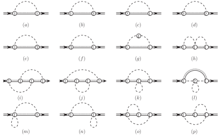
Figure 1: One and two-loop self-energy diagrams contributing to the width of the delta resonance up-to-and-including fifth order according to the standard power counting. The dashed and double solid lines represent the pions and the delta resonances, respectively. The double (solid-dotted) lines in the loops correspond to either nucleons or deltas. The numbers in the circles give the chiral orders of the vertices.

The complex pole position $z$ of the $\Delta$-propagator can be found by solving the equation

$$z-m_{\Delta}^{0}-\Sigma_{1}(z^{2})-z\,\Sigma_{6}(z^{2})\equiv z-m_{\Delta}^{0}-\Sigma(z)=0\,.$$ (3)

The pole mass and the width are defined by parameterizing the pole position $z$ as

$$z=m_{\Delta}-i\,\frac{\Gamma_{\Delta}}{2}\,.$$ (4)

The one- and two-loop self-energy diagrams contributing to the width of the delta resonance up to order $q^{5}$ are shown in Fig. 1, where the counterterm diagrams are not displayed. The underlying effective chiral Lagrangian of pions, nucleons and the delta resonances is given in the Appendix. For more details and the explicit discussion of the power counting, relevant for the current calculation of the delta width at leading two-loop order, we refer to Refs. Yao:2016vbz ; Gegelia:2016xcw .

We solve Eq. (3) perturbatively order by order in the loop expansion. For that purpose we write the self-energy as an expansion in the number of loops (which is equivalent to an expansion in $\hbar$)

$$\Sigma=\hbar\,\Sigma_{(1)}+\hbar^{2}\Sigma_{(2)}+{\cal O}(\hbar^{3})\,,$$ (5)

and obtain the following expression for the width (modulo higher order corrections)

$$\Gamma_{\Delta} = \hbar\,2i\,{\rm Im}\left[\Sigma_{(1)}(m_{\Delta})\right]$$ (6)

$$+ \hbar^{2}\,2i\,\biggl{\{}{\rm Im}\left[\Sigma_{(1)}(m_{\Delta})\right]{\rm Re}\left[\Sigma_{(1)}^{\prime}(m_{\Delta})\right]+{\rm Re}\left[\Sigma_{(1)}(m_{\Delta})\right]{\rm Im}\left[\Sigma_{(1)}^{\prime}(m_{\Delta})\right]\biggr{\}}$$

$$+ \hbar^{2}\,2i\,{\rm Im}\left[\Sigma_{(2)}(m_{\Delta})\right]+{\cal O}(\hbar^{3}).$$

To calculate the contributions of the one-loop self-energy diagrams to the width, specified in the first two lines of Eq. (6), we use the corresponding explicit expressions. For the two-loop contribution, i.e. the terms in the third line, we use the Cutkosky cutting rules, that is we relate it to the corresponding decay amplitude $A_{\Delta\to\pi N}$ via

$$\Gamma_{\Delta}=\frac{\left[(m_{\Delta}+m_{N})^{2}-M_{\pi}^{2}\right]\left[\left(m_{\Delta}^{2}-m_{N}^{2}-M_{\pi}^{2}\right)^{2}-4M_{\pi}^{2}m_{N}^{2}\right]^{3/2}}{{192}\pi m_{\Delta}^{5}}\,|A_{\Delta\to\pi N}|^{2}\,,$$ (7)

where we have parameterised the amplitude for the decay $\Delta_{\mu}^{i}(p_{i})\to\pi^{a}(q_{a})N(p_{f})$ as

$${\cal A}=\bar{u}_{N}(p_{f})\left\{A_{\Delta\to\pi N}\,q_{a}^{\mu}\xi_{ai}^{\frac{3}{2}}\right\}u_{\mu}(p_{i})\,.$$ (8)

The tree and one-loop diagrams contributing to the $\Delta\to\pi N$ decay up to order $q^{3}$ are shown in Fig. 2. See again Refs. Yao:2016vbz ; Gegelia:2016xcw for the details on the power counting of the amplitude and the total width of the resonance.

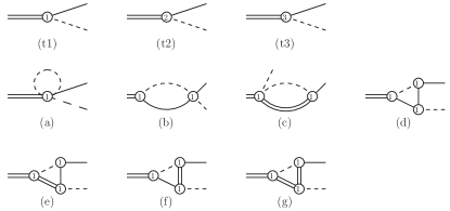
Figure 2: Feynman diagrams contributing to the decay $\Delta\to N\pi$ up to leading one-loop order. Dashed, solid and double lines represent pions, nucleons and delta resonances, respectively. Numbers in the circles mark the chiral orders of the vertices.

Calculating one- and two-loop contributions in the delta width as specified above we observe that by defining a linear combination of $\pi N\Delta$ couplings

$$h_{A}=h-\left(b_{3}\Delta_{23}+b_{8}\,\Delta_{123}\right)-\left(f_{1}\Delta_{23}+f_{2}\,\Delta_{123}\right)\Delta_{123}+2(2f_{4}-f_{5})M_{\pi}^{2}\,,$$ (9)

with

$$\Delta_{123}\equiv\frac{M_{\pi}^{2}+m_{N}^{2}-m_{\Delta}^{2}}{2m_{N}}\,,\qquad\Delta_{23}\equiv m_{N}-m_{\Delta}\,,$$ (10)

modulo higher order terms, the whole explicit dependence on the couplings $b_{3}$, $b_{8}$, $f_{1}$, $f_{2}$, $f_{4}$ and $f_{5}$ disappears from the expression of the delta width. This allows us to extract with a good accuracy the numerical value of $h_{A}$ from the experimental value of the delta width for a given value of the leading $\pi\Delta$ coupling constant $g_{1}$. Such a correlation between $\pi N\Delta$ and $\pi\Delta$ couplings exists in the large $N_{C}$ limit but, as far as we know, is observed here first for the real world with $N_{C}=3$.

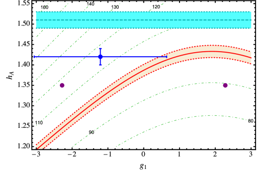
Figure 3: Value of the pion-nucleon-delta coupling $h_{A}$ as a function of the pion-delta coupling $g_{1}$ represented by the solid red line and the corresponding band given by the dashed red lines. The central line corresponds to $\Gamma_{\Delta}=100$ MeV, while the band is obtained by varying $\Gamma_{\Delta}$ in the range of $98-102$ MeV Agashe:2014kda . The dot-dashed lines correspond to various values of the delta width indicated by their values (in MeV). For comparison, the blue dot with error bars represents the real part of the coupling from Ref. Yao:2016vbz , the purple dots stand for the values of the leading order pion-nucleon-delta coupling obtained in the large-$N_{c}$ limit and the horizontal dashed line with cyan band corresponds to the value (with error represented by the band) from Ref. Bernard:2012hb .

We use the following standard values of the parameters Agashe:2014kda : $g_{A}=1.27$, $M_{\pi}=139\,$MeV, $m_{N}=939\,$MeV, $m_{\Delta}=1210\,$MeV, $F_{\pi}=92.2\,$MeV and obtain for the full decay width of the delta resonance

$$\Gamma_{\Delta} = 53.91\,{h}_{A}^{2}+0.87g_{1}^{2}{h}_{A}^{2}-3.31g_{1}{h}_{A}^{2}-0.99\,{h}_{A}^{4}.$$ (11)

Substituting $\Gamma_{\Delta}=100\pm 2\ {\rm MeV}$ from the PDG in Eq. (11), we extract $h_{A}$ as a function of $g_{1}$. The obtained result is plotted in Fig. 3. For comparison we also show the numerical value of the $\pi N\Delta$ coupling from Ref. Bernard:2012hb (extracted at leading one-loop order and thus independent of $g_{1}$), the one obtained by applying symmetry considerations in the large-$N_{C}$ limit and the real part of the same linear combination of the couplings, as in current work, fitted to the pion-nucleon scattering phase shifts of Ref. Yao:2016vbz , which uses a different renormalization scheme leading to a complex valued $h_{A}$. Note also that Ref. Hemmert:1997ye extracts 1.05 as the value of the leading order $\pi N\Delta$ coupling in the heavy baryon approach.

To summarize, in the current work we have calculated the width of the delta resonance up to leading two-loop order in baryon chiral perturbation theory. Using the obtained results we fixed a combination of pion-nucleon-delta couplings, which also contributes in the pion nucleon scattering process, as a function of the leading pion-delta coupling.

Appendix A Effective Lagrangian

Here, we list the relevant terms of the chiral effective Lagrangian with pions, nucleons and deltas contributing to our calculation:

$${\cal L}_{\pi N}^{(1)} = \bar{\Psi}_{N}\left\{i\not{D}-m+\frac{1}{2}g\,\not{u}\gamma^{5}\right\}\Psi_{N}\,,$$

$${\cal L}^{(1)}_{\pi\Delta} = -\bar{\Psi}_{\mu}^{i}\xi^{\frac{3}{2}}_{ij}\left\{\left(i\not{D}^{jk}-m_{\Delta 0}\delta^{jk}\right)g^{\mu\nu}-i\left(\gamma^{\mu}D^{\nu,jk}+\gamma^{\nu}D^{\mu,jk}\right)+i\gamma^{\mu}\not{D}^{jk}\gamma^{\nu}+m_{\Delta 0}\delta^{jk}\gamma^{\mu}\gamma^{\nu}\right.$$

$$\left.+\frac{g_{1}}{2}\not{u}^{jk}\gamma_{5}g^{\mu\nu}+\frac{g_{2}}{2}(\gamma^{\mu}u^{\nu,jk}+u^{\nu,jk}\gamma^{\mu})\gamma_{5}+\frac{g_{3}}{2}\gamma^{\mu}\not{u}^{jk}\gamma_{5}\gamma^{\nu}\right\}\xi^{\frac{3}{2}}_{kl}{\Psi}_{\nu}^{l}\,,$$

$${\cal L}^{(1)}_{\pi N\Delta} = h\,\bar{\Psi}_{\mu}^{i}\xi_{ij}^{\frac{3}{2}}\Theta^{\mu\alpha}(z_{1})\ \omega_{\alpha}^{j}\Psi_{N}+{\rm h.c.}\,,$$

$${\cal L}^{(2)}_{\pi N\Delta} = \bar{\Psi}_{\mu}^{i}\xi_{ij}^{\frac{3}{2}}\Theta^{\mu\alpha}(z_{2})\left[i\,b_{3}\omega_{\alpha\beta}^{j}\gamma^{\beta}+i\,\frac{b_{8}}{m}\omega_{\alpha\beta}^{j}i\,D^{\beta}\right]\Psi_{N}+h.c.\ ,$$

$${\cal L}^{(3)}_{\pi N\Delta} = \bar{\Psi}_{\mu}^{i}\xi_{ij}^{\frac{3}{2}}\Theta^{\mu\nu}(z_{3})\left[\frac{f_{1}}{m}[D_{\nu},\omega_{\alpha\beta}^{j}]\gamma^{\alpha}i\,D^{\beta}-\frac{f_{2}}{2m^{2}}[D_{\nu},\omega_{\alpha\beta}^{j}]\{D^{\alpha},D^{\beta}\}\right.$$ (12)

$$\hskip 71.13188pt\left.+f_{4}\omega_{\nu}^{j}\langle\chi_{+}\rangle+f_{5}[D_{\nu},i\chi_{-}^{j}]\right]\Psi_{N}+h.c.,$$

where $\Psi_{N}$ and $\Psi_{\nu}$ are the isospin doublet field of the nucleon and the vector-spinor isovector-isospinor Rarita-Schwinger field of the $\Delta$-resonance with bare masses $m$ and $m_{\Delta 0}$, respectively. $\xi^{\frac{3}{2}}$ is the isospin-$3/2$ projector, $\omega_{\alpha}^{i}=\frac{1}{2}\,\langle\tau^{i}u_{\alpha}\rangle$ and $\Theta^{\mu\alpha}(z)=g^{\mu\alpha}+z\gamma^{\mu}\gamma^{\nu}$. Using field redefinitions the off-shell parameters $z$ can be absorbed in LECs of other terms of the effective Lagrangian and therefore they can be chosen arbitrarily Tang:1996sq ; Krebs:2009bf . We fix the off-shell structure of the interactions with the delta by adopting $g_{2}=g_{3}=0$ and $z_{1}=z_{2}=z_{3}=0$. For vanishing external sources, the covariant derivatives are given by

$$D_{\mu}\Psi_{N} = \left(\partial_{\mu}+\Gamma_{\mu}\right)\Psi_{N}\,,\ \ \Gamma_{\mu}=\frac{1}{2}\,\left[u^{\dagger}\partial_{\mu}u+u\partial_{\mu}u^{\dagger}\right]=\tau_{k}\Gamma_{\mu,k},$$

$$\left(D_{\mu}\Psi\right)_{\nu,i} = \partial_{\mu}\Psi_{\nu,i}-2\,i\,\epsilon_{ijk}\Gamma_{\mu,k}\Psi_{\nu,j}+\Gamma_{\mu}\Psi_{\nu,i}\,.$$ (13)

References

(1)
S. Weinberg,
Physica A96, 327 (1979).
(2)
J. Gasser and H. Leutwyler,
Annals Phys. 158, 142 (1984).
(3)
J. Gasser, M. E. Sainio, and A. Švarc,
Nucl. Phys. B307, 779 (1988).
(4)
E. E. Jenkins and A. V. Manohar,
Phys. Lett. B 255, 558 (1991).
(5)
V. Bernard, N. Kaiser, J. Kambor and U.-G. Meißner,
Nucl. Phys. B 388, 315 (1992).
(6)
V. Bernard, N. Kaiser and U.-G. Meißner,
Int. J. Mod. Phys. E 4, 193 (1995).
(7)
H. B. Tang,
arXiv:hep-ph/9607436.
(8)
T. Becher and H. Leutwyler,
Eur. Phys. J. C 9, 643 (1999).
(9)
J. Gegelia and G. Japaridze,
Phys. Rev. D 60, 114038 (1999).
(10)
T. Fuchs, J. Gegelia, G. Japaridze, and S. Scherer,
Phys. Rev. D 68, 056005 (2003).
(11)
T. R. Hemmert, B. R. Holstein, and J. Kambor,
J. Phys. G 24, 1831 (1998).
(12)
V. Pascalutsa and D. R. Phillips,
Phys. Rev. C 67, 055202 (2003).
(13)
V. Bernard, T. R. Hemmert, and U.-G. Meißner,
Phys. Lett. B 565, 137 (2003).
(14)
V. Pascalutsa, M. Vanderhaeghen, and S. N. Yang,
Phys. Rept. 437, 125 (2007).
(15)
C. Hacker, N. Wies, J. Gegelia, and S. Scherer,
Phys. Rev. C 72, 055203 (2005).
(16)
D. L. Yao, D. Siemens, V. Bernard, E. Epelbaum, A. M. Gasparyan, J. Gegelia, H. Krebs and U.-G. Meißner,
JHEP 1605, 038 (2016).
(17)
J. Gegelia, U.-G. Meißner and D. L. Yao,
Phys. Lett. B (2016). [arXiv:1606.04873 [hep-ph]].
doi:10.1016/j.physletb.2016.07.068
(18)
K. A. Olive et al. [Particle Data Group Collaboration],
Chin. Phys. C 38, 090001 (2014).
(19)
V. Bernard, E. Epelbaum, H. Krebs and U.-G. Meißner,
Phys. Rev. D 87, 054032 (2013).
(20)
H. B. Tang and P. J. Ellis,
Phys. Lett. B 387, 9 (1996).
(21)
H. Krebs, E. Epelbaum and U.-G. Meißner,
Phys. Lett. B 683, 222 (2010).