Where does a random process hit a fractal barrier?

Abstract.

Given a Brownian path $\beta(t)$ on ${\mathbb{R}}$, starting at $1$, a.s. there is a singular time set $T_{\beta}$, such that the first hitting time of $\beta$ by an independent Brownian motion, starting at $0$, is in $T_{\beta}$ with probability one. A couple of problems regarding hitting measure for random processes are presented.

1. Introduction

The study of Harmonic (or hitting) measure for Brownian motion is a well developed subject with dramatic achievements and major problems which are still wide open, see  [4]. In this note we present a couple of problems regarding hitting measure for a wider class of random processes and obtain one result.

When does one dimensional Brownian motion starting at $0$, hits an independent Brownian motion starting at $1$, which serves as the barrier?

We show that conditioning on the barrier, a.s. with respect to the Wiener measure on barriers, there is a singular time set (which is a function of the barrier only) that a.s. contains the first hitting time of the barrier.

2. Random processes in the plane

Let $\gamma$ be an unbounded one sided curve in the Euclidean plane. Given a simply connected open bounded domain $\Omega$ in the plane. Reroot the origin of $\gamma$ at a uniformly chosen point of $\Omega$, and rotate $\gamma$ with an independent uniformly chosen angel, around it’s root. Look at the hitting point of this random translation and rotation of $\gamma$ on the boundary of the domain $\partial\Omega$. For every root in $\Omega$ the hitting point maps the uniform measure on directions $U[0,2\pi]$ to a measure on $\partial\Omega$.

Conjecture 2.1.

For any $\gamma$ and $\Omega$, for almost every root, the corresponding measure on $\partial\Omega$ has $0$ two dimensional Lebesgue measure.

Moreover,

Question 2.2.

For any $\gamma$ and $\Omega$, for almost every root, the corresponding measure on $\partial\Omega$ has Hausdorff dimension (at most) one?

It is of interest to prove even that dimension drops below $2$. Or better below the dimension of $\partial\Omega$ when it is strictly above $1$. Also getting the result for a restricted family of curves, is of interest. If $\gamma$ is a Brownian path then Makarov’s theorem [7] gives an affirmative answer. For partial results on this conjecture when $\gamma$ is a straight line see  [3].

2.1. Simple random walks on discrete fractals

By Makarov’s theorem [7] (and Jones and Wolff  [5] for general domains) and it’s adaptation by Lawler [6] via coupling to simple random walk, it is know that the dimension of the hitting measure for two dimensional Brownian motion drops to (at most) $1$. We therefore suspect that harmonic measure for simple random walk on self similar planar fractals will also be at most $1$. Here is a specific formulation.

2.1.1. Sierpinski gasket

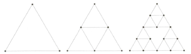
Figure 1. The first three generation of Sierpinski gasket graphs sequence.

Given a subset $S$ of the vertices in the $n$-th generation of the Sierpinski gasket graph sequence (see Figure 1).

Question 2.3.

Show that the entropy of the hitting measure for a simple random walk starting at the top vertex on $S$ is at most $n$.

Note that in the $n$-th generation Sierpinski gasket graph, the size of the bottom side is $2^{n-1}+1$, which we believe realizes the largest entropy possible. (Entropy in base $2$, $-\sum_{i}p_{i}\log_{2}p_{i}$).

2.2. Fractional BM

Recall the probability Brownian motion in ${\mathbb{R}}^{2}$, starting at $(1,0)$ hits the negative $x$-axis first at $[-\epsilon,0]$ behaves like $\epsilon^{1/2}$, as epsilon goes to $0$.

We would like to have a natural statement along the lines that the rougher the process starting at $(1,0)$ the larger the probability it will hit the negative $x$-axis first near the tip. E.g. if the process starting at $(1,0)$ is a two dimensional fBM with Hurst parameter $H$, then as $H$ decreases the probability it hits the $\epsilon$ tip is growing (maybe it is about $\epsilon^{H}$ ?)

One can ask similar a question for the graph of one dimensional fBM and SLE curves.

3. Random process on the line

Theorem 3.1.

Let $B$ and $W$ be independent standard Brownian motions on ${\mathbb{R}}$, and let $\sigma,c>0$. Define $\tau$ to be the first time when $B$ hits the barrier $c+\sigma W$, i.e.

$$\tau:=\inf\{t\mid B_{t}=c+\sigma W_{t}\}.$$

Then conditionally on $W$, the distribution of $\tau$ is almost surely singular to the Lebesgue measure.

In the proof we will make use of the following standard fact from measure theory.

Proposition 3.2.

Let $M,N$ be probability measures on $X\times Y$, a product of standard Borel spaces. Consider the disintegration of $M,N$ with respect to the $X$-variable (i.e. with respect to the canonical projection $X\times Y\to X$). We write it as follows:

$$M(dx,dy)=M_{X}(dx)M_{Y\mid X}(x,dy)$$

$$N(dx,dy)=N_{X}(dx)N_{Y\mid X}(x,dy)$$

where $M_{X}$ (resp. $N_{X}$) is the pushforward of $M$ (resp $N$) under $X\times Y\to X$, and $M_{Y\mid X}(x)$ (resp. $N_{Y\mid X}(x)$) is corresponding conditional of $y$ given $x$. Assume that $M_{X}$ is equivalent (i.e. mutually absolutely continuous) to $N_{X}$. Then the following are equivalent:

1. $M$ is singular to $N$

2. $M_{Y\mid X}(x)$ is singular to $N_{Y\mid X}(x)$ for $M_{X}$-almost all $x$

Another fact we will need is the Bessel(3)-like behavior of the Brownian motion immediately before hitting a constant barrier. This is an immediate consequence of Williams’ Brownian path decomposition theorem (e.g. Theorem VII.4.9 in [8]).

Proposition 3.3.

Consider a Brownian motion $B$ starting from $0$, and let $c>0$. Let $\tau$ be the hitting time $\tau:=\inf{t\mid B_{t}=c}$. Then for any $\varepsilon>0$ the conditional distribution of $(c-B_{T-s})_{s=0}^{T-\varepsilon}$ conditioned on $\tau=T>\varepsilon$ is equivalent to that of a Bessel(3) process starting from $0$ restricted to the time interval $[0,T-\varepsilon]$.

Proof of Theorem 3.1.

Consider the random measure $\delta_{\tau}$ and $D:=\mathbb{E}[\delta_{\tau}\mid W]$. The latter is exactly the conditional distribution of $\tau$ given $W$. By Proposition 3.2 (applied to $X:=\Omega$, $Y:={\mathbb{R}}$), almost sure singularity of $D=D(\omega,dt)$ to the (determinstic) Lebesgue measure is equivalent to the singularity of $\mathbb{P}(d\omega)D(\omega,dt)$ to $\mathbb{P}(d\omega)dt$. On the other hand, the two spaces $X$ and $Y$ in Proposition 3.2 play symmetric roles, so instead one may disintegrate with respect to the $t\in{\mathbb{R}}$ variable. More precisely, let $\Pi(t,d\omega)$ (resp. $\pi(t,d\omega)$) be the disintegration of $\mathbb{P}(d\omega)D(\omega,dt)$ (resp. $\mathbb{P}(d\omega)\delta_{\tau}(\omega,dt)$) with respect to $t$. Then the $\mathbb{P}$-almost sure singularity of $D$ with respect to the Lebesgue measure is equivalent to the singularity of $\Pi(t)$ with respect to $\mathbb{P}$ for Lebesgue-almost all $t$. On the other hand, the measures $\mathbb{P}(d\omega)D(\omega,dt)$ and $\mathbb{P}(d\omega)\delta_{\tau}(\omega,dt)$ agree when restricted to the $\sigma$-algebra $\sigma(W)\otimes\mathrm{Borel}({\mathbb{R}})$; therefore, $\Pi(t)$ and $\pi(t)$ agree on $\sigma(W)$ for Lebesgue-almost all $t$. Since $D$ is measurable with respect to $\sigma(W)$, it is enough to verify that $\pi(t)$ is singular to $\mathbb{P}$ when restricted to $\sigma(W)$.

Using Proposition 3.3 we can characterize $\pi(t)$ explicitly, at least up to equivalence. Indeed, the time when $B$ hits $c+\sigma W$ is exactly the time when

$$X:=\frac{1}{\sqrt{1+\sigma^{2}}}B-\frac{\sigma}{\sqrt{1+\sigma^{2}}}W,$$

which is itself a standard Brownian motion under $\mathbb{P}$, hits the constant barrier $\tilde{c}:=\frac{c}{\sqrt{1+\sigma^{2}}}$. Thus by Proposition 3.3, the distribution of $\tilde{c}-X_{t-\cdot}$ under $\pi(t)$ is (locally) equivalent to Bessel(3). On the other hand,

$$Y:=\frac{\sigma}{\sqrt{1+\sigma^{2}}}B+\frac{1}{\sqrt{1+\sigma^{2}}}W$$

is $\mathbb{P}$-independent of $X$, and since the $\tau$ is measurable with respect to $X$, the independent part $Y$ is not affected by our change of measure. Thus under $\pi(t)$, $X$ and $Y$ are still independent, and $Y_{t-\cdot}$ remains (locally) equivalent to a Brownian motion.

In order to prove the singularity result we only need the restriction of our measures to $\sigma(W)$. Since

$$W=-\frac{\sigma}{\sqrt{1+\sigma^{2}}}X+\frac{1}{\sqrt{1+\sigma^{2}}}Y,$$

we see that under $\pi(t)$, $W_{t-\cdot}$ is locally equivalent to a combination of a Bessel(3) and an independent Brownian motion. Under $\Pi$, however, it is locally a Brownian motion. Thus the problem reduces to the proving that the local behaviour at time zero of the sum of independent processes

$$U\sim\alpha\cdot\mathrm{BES(3)}+\sqrt{1-\alpha^{2}}\cdot\mathrm{BM}$$

is almost surely distinguishable from that of $V\sim\mathrm{BM}$, where $\alpha=-\frac{\sigma}{\sqrt{1+\sigma^{2}}}<0$. This can be achieved by, say, noting that these processes satisfy a law of iterated logarithm with different almost sure constants. Namely,

$$\limsup_{s\to 0}\frac{V_{s}}{\sqrt{2s\log\log s}}=1$$

$$\limsup_{s\to 0}\frac{U_{s}}{\sqrt{2s\log\log s}}\leq\sqrt{1-\alpha^{2}}<1$$

∎

Question 3.4.

Study this phenomena for larger class of barriers, e.g. iterated function systems. Give sharper bounds on the dimension of the the set which a.s. contains the hitting time.

To study this for iterated function systems, we need a uniform bound on the radon nikodym derivative of the harmonic measure with respect to the uniform measure, at all scales.

Here is a formulation of this problem for random fields. Consider a function from ${\mathbb{R}}^{d}$ to ${\mathbb{R}}^{n}$ as a barrier, and look when a random field indexed by ${\mathbb{R}}^{d}$ hits the barrier, where the hitting index is defined say as the index with the smallest $L_{2}$ norm.

4. Further comments

• Bourgain’s proof

  Bourgain [2] proved a dimension drop result for Brownian motion in ${\mathbb{R}}^{d}$ for any $d$. Two properties of BM are used in the clever argument, uniform Harnack inequality at all scales and the Markov property, to get independent between scales. These two properties hold for a wider set of processes in a larger set of spaces, (e.g. Brownian motion on nilpotent groups and fractals). Also weaker forms of these properties are sufficient to get some drop.

• Random walk on graphs

  This note concerns with harmonic measure in ”small spaces” of dimension at most two. See  [1] for a study of hitting measure for the simple random walk in the presence of a spectral gap: on highly connected graphs such as expanders, simple random walk is mixing fast and it is shown that it hits the boundary of sets in a rather uniform way. More involved behavior arises for graphs which are neither polynomial in the diameter nor expanders, see  [1].

• Let’s play

  Rules: each of the $k\geq 2$ players picks independently a unit length path (not necessarily a segment) in the Euclidean plane that contains the origin. Let $S$ be the union of all the $k$ paths. Look at the harmonic measure from infinity on $S$. The winner is the player that his path, gets the maximal harmonic measure.

  Is choosing a segment from the origin to a random point on the unit circle, independently by each of the players, a Nash equilibrium?

References

- [1] I. Benjamini and A. Yadin. Harmonic measure in the presence of a spectral gap. Annales Institut Henri Poincare. 52, 1050-–1060, 2016.
- [2] J. Bourgain. On the Hausdorff dimension of harmonic measure in higher dimension. Invent. Math. 87, 477–-483, 1987.
- [3] K. Falconer and J. Fraser, The visible part of plane self-similar sets. Proc. Amer. Math. Soc. 141, 269-–278, 2013.
- [4] J. Garnett and D. Marshall. Harmonic measure, volume 2. Cambridge University Press, 2005.
- [5] P. Jones and T. Wolff. Hausdorff dimension of harmonic measures in the plane. Acta Mathematica. 161, 131–-144, 1988.
- [6] G. Lawler. A discrete analogue of a theorem of Makarov. Combin. Probab. Comput. 2, 181–-199, 1993
- [7] N. Makarov. On the distortion of boundary sets under conformal mappings. Proc. London Math. Soc. 3, 369-–384, 1985.
- [8] D. Revuz and M. Yor. Continuous martingales and Brownian motion. Springer, 1999