Double quantum dot Cooper-pair splitter at finite couplings

Abstract

We consider the sub-gap physics of a hybrid double-quantum dot Cooper-pair splitter with large single-level spacings, in the presence of tunnelling between the dots and finite Coulomb intra- and inter-dot Coulomb repulsion. In the limit of a large superconducting gap, we treat the coupling of the dots to the superconductor exactly. We employ a generalized master-equation method which easily yields currents, noise and cross-correlators. In particular, for finite inter- and intra-dot Coulomb interaction, we investigate how the transport properties are determined by the interplay between local and nonlocal tunneling processes between the superconductor and the dots. We examine the effect of inter-dot tunneling on the particle-hole symmetry of the currents with and without spin-orbit interaction. We show that spin-orbit interaction in combination with finite Coulomb energy opens the possibility to control the nonlocal entanglement and its symmetry (singlet/triplet). We demonstrate that the generation of nonlocal entanglement can be achieved even without any direct nonlocal coupling to the superconducting lead.

I Introduction

Recent developments in quantum technologiesMonroe (2002); Martinis (2009); Ladd et al. (2010) have shown an enormous potential for applications. Quantum key distributions in quantum cryptographyLo et al. (2014) have became almost a standard technology. This progress was mainly realized in optical systems. In order to enable the full potential of quantum technologies, spintronicsLinder and Robinson (2015) and topotronics,Yoshimi et al. (2015) in solid state systems, it is crucial to be able to generate entangled states. A promising route to entanglement generation is offered by hybrid superconducting nanostructures. This type of system has very reach physics. For example, the possibility to emulate topological superconductors in low dimensions with, possibly, the creation of Majorana bound states has clearly shown a revolutionary potential.Qi and Zhang (2011); Kitaev (2001); Nayak et al. (2008); Alicea (2012) The enormous advancement in the production and control of nanotubes and nanowiresRomeo et al. (2012); Rossella et al. (2014) opened up the possibility to couple nanosystems, in a very controlled way, to superconductorsGiazotto et al. (2011); Roddaro et al. (2011); Spathis et al. (2011) taking advantage of their properties such as the spin-orbit (SO) interaction. Quantum phase transitions and anomalous current-phase relations have been studied in hybrid semiconductor-superconductor devices.Lee et al. (2014); Yokoyama et al. (2014); Mironov et al. (2015); Žonda et al. (2015); Marra et al. (2016) SO interaction in the presence of superconducting correlations may lead to the generation of triplet ordering in nanowiresShekhter et al. (2016) or quantum wells.Yu and Wu (2016)

Superconductors are a natural source of electron-singlets (Cooper-pairs) which may provide nonlocal entangled electrons when split.Bouchiat et al. (2003); Russo et al. (2005); Schindele et al. (2012); Fülöp et al. (2014); Linder and Robinson (2015) Semiconductor-superconductor-hybrid devices have been the object of experimental studies investigating signatures of nonlocal transport in charge currents and cross-correlations.Das et al. (2012); Schindele et al. (2014); He et al. (2014)

Cooper-pair splitting has also been investigated in Josephson junctions.Ishizaka et al. (1995); Deacon et al. (2015) Spin entanglementRecher et al. (2001); Sothmann et al. (2014) and electron transportHammer et al. (2007); Chevallier et al. (2011); Rech et al. (2012); Droste et al. (2012); Trocha and Weymann (2015) in hybrid systems have been theoretically studied using full counting statistics (FCS)Belzig and Samuelsson (2003); Governale et al. (2008); Morten et al. (2008); Droste et al. (2012); Futterer et al. (2013); Soller and Komnik (2014); Stegmann and König . Further studies have investigated the effects of external magnetic fieldsFülöp et al. (2015) and thermal gradientsMachon et al. (2013); Cao et al. (2015) on Cooper-pair splitting. Quantum dots increase the efficiency of Cooper-pair splitting since sufficiently large intradot Coulomb interaction suppresses local Cooper-pair tunneling.Recher et al. (2001); Hofstetter et al. (2009); Schindele et al. (2012, 2014); Fülöp et al. (2015) Alternatively, the efficiency can be improved using spin-filtering as in spin valves.Beckmann et al. (2004); Samm et al. (2014) Typically all these systems are investigated assuming a very strong on-site Coulomb interaction. In the present paper, we consider the possibility of a weak Coulomb interaction which complicates the analysis as it introduces additional transport channels. We find that this is not necessarily a limitation in the creation of nonlocal entanglement, instead it offers a different route to achieve nonlocal entanglement.

The model studied in this paper is a Cooper-pair splitter based on a double quantum dot (DQD) circuit that is tunnel coupled to one superconductor and to two normal leads, see Fig 1. This is an extension of the model studied by Eldridge et al., Ref. Eldridge et al., 2010, to finite interdot tunneling and SO interaction. In this work, we investigate the effect of both local and nonlocal Cooper-pair tunneling on the current and conductance in the presence of finite Coulomb energies. Finally, we will discuss how interdot tunneling with or without SO interaction affects the generation of nonlocal entanglement.

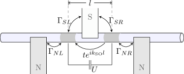
Figure 1: Double quantum dot circuit coupled to a $s$-wave superconductor acting as a Cooper-pair splitter. Electron-singlets nonlocally injected by the superconductor ($S$) into the double quantum dot can leave the system through opposite normal leads ($N$). Hence this system can be operated as a source of nonlocal entangled electron pairs.

This work is organized as follows. In section II we introduce the model and the formalism employed for our calculations. In Section III we provide an overview of the transport properties in the absence of inter-dot tunneling. The effect of interdot tunneling and SO interaction is discussed in section IV . Finally, section V is devoted to conclusions.

II Model and master-equation

II.1 Model of the hybrid double quantum-dot system

The system under consideration, depicted schematically in Fig. 1, consists of two quantum dots tunnel coupled to a common $s$-wave superconductor and each individually to a separate normal lead.Schindele et al. (2012, 2014) The double-quantum-dot (DQD) system is modelled by the Hamiltonian

$$H_{\textrm{DQD}}={} \sum_{\alpha,\sigma}\epsilon_{\alpha}n_{\alpha\sigma}+\sum_{\alpha}U_{\alpha}n_{\alpha\uparrow}n_{\alpha\downarrow}+U\sum_{\sigma,\sigma^{\prime}}n_{L\sigma}n_{R\sigma^{\prime}}$$

$$+\Big{(}\frac{t}{2}\sum_{\sigma}e^{\operatorname{sgn}(\sigma)i\phi}d^{\dagger}_{L\sigma}d_{R\sigma}+\mathrm{H.c.}\Big{)},$$ (1)

where $\alpha=L,R$ labels the left and right dot, respectively, and $\sigma=\uparrow,\downarrow$ denotes the spin. The orbital levels $\epsilon_{\alpha}$ are spin degenerate, and $U_{\alpha}$ and $U$ denote the intra- and interdot Coulomb interaction, respectively. We define the number operator $n_{\alpha\sigma}=d_{\alpha\sigma}^{{\dagger}}d_{\alpha\sigma}$, where $d_{\alpha\sigma}$ is the annihilation operator for an electron with spin $\sigma$ in dot $\alpha$. The last term in Eq. (1) describes interdot tunneling through a barrier with SO coupling.Droste et al. (2012) The phase $\phi$ is the phase acquired by a spin-up electron when tunneling from the right dot to the left one and it can be expressed as $\phi\equiv k_{\textrm{SO}}l\neq 0$ where the SO strength is measured in terms of the wave number $k_{\textrm{SO}}$, $l$ is the interdot distance. Here, we used the convention $\operatorname{sgn}(\uparrow)=+1$ and $\operatorname{sgn}(\downarrow)=-1$. The SO coupling may become relevant for InAsFasth et al. (2007); Estévez Hernández et al. (2010) and InSbNadj-Perge et al. (2012); van Weperen et al. (2015) nanowire devices where one finds values of $1/k_{\text{SO}}$ of typically 50-300 nm which are comparable to the typical distance between the two dots in these nanodevices. The model Hamiltonian, Eq. (1), gives an accurate description of the system when the single-particle level spacings in the dots are large compared to the other energy scales. In this limit, for $k_{B}T\ll U_{\alpha}$, at most 4 electrons can occupy the double-quantum-dot system.

The normal leads ($\eta=L,R$) are modeled as fermionic baths while the superconducting lead ($\eta=S$) is described by the mean-field $s$-wave BCS Hamiltonian,

$$H_{\eta}=\sum_{k\sigma}\epsilon_{\eta k}c_{\eta k\sigma}^{\dagger}c_{\eta k\sigma}-\delta_{\eta,S}\Delta\sum_{k}\big{(}c_{\eta-k\downarrow}c_{\eta k\uparrow}+\mathrm{H.c.}\big{)}.$$ (2)

Here, $c_{\eta k\sigma}$ ($c_{\eta k\sigma}^{\dagger}$) are the fermionic annihilation (creation) operators of the leads and $\epsilon_{\eta k}$ are corresponding single-particle energies. Without loss of generality the pair potential in the superconductor, $\Delta$, is chosen to be real and positive. For convenience, we choose the chemical potential of the superconductor to be zero and use it as reference for the chemical potentials of the normal leads.

The quantum dots are coupled to the normal leads and the superconductor via the Hamiltonian, $H_{\textrm{DQD-leads}}=\sum_{\eta\alpha}H^{\textrm{tunnel}}_{\eta\alpha}$, where the coupling of dot $\alpha$ with lead $\eta=L,R,S$ is described by the standard tunneling Hamiltonian

$$H^{\textrm{tunnel}}_{\eta\alpha}=\sum_{k\sigma}\big{(}V_{\eta\alpha}c^{\dagger}_{\eta k\sigma}d_{\alpha\sigma}+\mathrm{H.c.}\big{)}.$$ (3)

Here, $V_{LR}=V_{RL}=0$ since the left (right) dot is not directly coupled to the right (left) lead. The effective tunneling rates are $\Gamma_{\eta\alpha}=(2\pi/\hbar)|V_{\eta\alpha}|^{2}\rho_{\eta}$ where the density of states $\rho_{\eta}$ in lead $\eta$ is assumed to be energy independent in the energy window relevant for the transport. For a better readability we introduce $\Gamma_{N\alpha}\equiv\Gamma_{\alpha\alpha}$ to emphasize the coupling to the normal leads with a subscript $N$.

As we are interested in Cooper-pair splitting and in general sub-gap transport, we assume the superconducting gap to be the largest energy scale in the system. In this limit the quasi-particles in the superconductor are inaccessible and the superconducting lead can be traced out exactly.Rozhkov and Arovas (2000); Meng et al. (2009); Rajabi et al. (2013) Thus, the system dynamics reduces to the effective HamiltonianEldridge et al. (2010); Braggio et al. (2011); Sothmann et al. (2014)

$$\begin{split}H_{S}=H_{\textrm{DQD}}&-\sum_{\alpha=L,R}\frac{\Gamma_{S\alpha}}{2}\big{(}d^{\dagger}_{\alpha,\uparrow}d^{\dagger}_{\alpha,\downarrow}+\mathrm{H.c.}\big{)}\\ &-\frac{\Gamma_{S}}{2}\big{(}d^{\dagger}_{R,\uparrow}d^{\dagger}_{L,\downarrow}-d^{\dagger}_{R,\downarrow}d^{\dagger}_{L,\uparrow}+\mathrm{H.c.}\big{)}\end{split}$$ (4)

where $\Gamma_{S}$ describes the nonlocal proximity effect. This nonlocal coupling decays with the interdot distance $l$, as $\Gamma_{S}\sim\sqrt{\Gamma_{SL}\Gamma_{SR}}e^{-l/\xi}$, with $\xi$ being the coherence length of the Cooper-pairs.Recher et al. (2001) So, only values $0\leq\Gamma_{S}\leq\sqrt{\Gamma_{SL}\Gamma_{SR}}$ are physically admissible. The second term describes the local Andreev reflection (LAR) processes where Cooper pairs tunnel locally from the superconductor to dot $\alpha$. The last term describes cross-Andreev reflection (CAR), that is a nonlocal Cooper-pair tunneling process where Cooper-pairs split into the two dots. Due to CAR, electrons leaving the system through opposite normal leads are potentially entangled. On the contrary, the LAR process does not contribute to the nonlocal entanglement production. The LAR process is usually attenuated by large intradot couplings, $U_{\alpha}$.

Albeit the effective Hamiltonian, Eq. (4), no longer preserves the total particle number for the double-dot system it still preserves the parity of the total occupation, $\sum_{\alpha\sigma}n_{\alpha\sigma}$. A decomposition, $H_{S}=H_{S}^{\textrm{even}}\oplus H_{S}^{\textrm{odd}}$, of the system Hamiltonian into an even and an odd parity sector is provided in Appendix A. In conclusion the Hilbert space for the proximized double-dot system has the dimension 16. A generalization to include more charge states, to treat for instance smaller level spacings or higher temperatures, is straightforward and can be treated within the master-equation approach presented below. Lowest order corrections in $1/\Delta$ can be also included in the system Hamiltonian according to Ref. Amitai et al., 2016.

In the following, we consider the case of the quantum dots weakly coupled to the normal leads in comparison to the superconducting one, $\Gamma_{S\alpha}\gg\Gamma_{N\alpha^{\prime}}$. In this limit quantum transport is mainly characterized by the transitions between the eigenstates of $H_{S}$, the Andreev bound states.Eldridge et al. (2010); Braggio et al. (2011) Those tunneling events with the normal leads either add a single charge to the DQD or remove one from it and, thus, change the parity of the DQD.

II.2 Master-equation and transport coefficients

We calculate the stationary transport properties, such as the current and the conductance, by means of the master-equation formalism using standard FCS techniques. All the relevant transport properties can be related to the Taylor coefficients of the cumulant generating functionBagrets and Yu. V. Nazarov (2003); Flindt et al. (2004); Braggio et al. (2006); Kaiser and Kohler (2007); Hussein and Kohler (2014) and obtained in an iterative scheme.Flindt et al. (2008, 2010) In this work, we limit our analysis to the current and the differential conductance, however, also higher cumulants, such as noise and cross-correlations, can be easily obtained.

Here, we consider the regime $\Gamma_{N\alpha}\ll k_{B}T$, for which the tunnel couplings to the normal leads can be treated in first order. The tunnel couplings to the superconductor, the charging energies, and the interdot tunneling are treated exactly within the model under consideration. This leads to the master-equation $\dot{P}_{a}=\sum_{a^{\prime}}\big{(}w_{a\leftarrow a^{\prime}}P_{a^{\prime}}-w_{a^{\prime}\leftarrow a}P_{a}\big{)}$ for the occupation probabilities $P_{a}$ of the eigenstates $|a\rangle$ of the system Hamiltonian, where $w_{a\leftarrow a^{\prime}}$ are Fermi golden rule rates. The tunneling rates for the tunneling-in contribution read

$$w_{a\leftarrow a^{\prime}}^{\alpha\sigma,\textrm{in}}({\bm{\chi}})=e^{-i\chi_{\alpha}}\Gamma_{N\alpha}f_{\alpha}(E_{a}-E_{a^{\prime}})|\langle a|d_{\alpha\sigma}^{\dagger}|a^{\prime}\rangle|^{2}.$$ (5)

Here, $E_{a}$ and $|a\rangle$ refer to the eigenenergies and the eigenstates of $H_{S}$, and $f_{\alpha}(\epsilon)=\{1+\exp[(\epsilon-\mu_{\alpha})/k_{B}T]\}^{-1}$ denotes the Fermi function of normal lead $\alpha$ with chemical potential $\mu_{\alpha}$ and temperature $T$. We only attachBagrets and Yu. V. Nazarov (2003); Braggio et al. (2006) counting variables to the normal leads, ${\bm{\chi}}=(\chi_{L},\chi_{R})$. The stationary current through the superconductor $I_{S}$, can be easily expressed in terms of the currents through the left and right leads, $I_{S}=-I_{L}-I_{R}$. The tunneling-out contribution can be obtained from the substitution $\{d_{\alpha\sigma}^{\dagger},f_{\alpha}(\epsilon),\chi_{\alpha}\}\to\{d_{\alpha\sigma},\bar{f}_{\alpha}(-\epsilon),-\chi_{\alpha}\}$, where $\bar{f}_{\alpha}(\epsilon)=1-f_{\alpha}(\epsilon)$. Summation over the spin and lead indices yields the full rates $w_{a\leftarrow a^{\prime}}=\sum_{\alpha\sigma}(w_{a\leftarrow a^{\prime}}^{\alpha\sigma,\textrm{in}}+w_{a\leftarrow a^{\prime}}^{\alpha\sigma,\textrm{out}})$.

Single electron tunneling changes the parity of the system. So, the only transitions that occur are between the eigenstates $|e_{i}\rangle$ of $H_{S}$ with even occupation number and those with odd occupation numbers, $|o_{j}\rangle$.

$|0\rangle$		empty state
$|S\rangle$	$=\frac{1}{\sqrt{2}}\big{(}d^{\dagger}_{R\uparrow}d^{\dagger}_{L\downarrow}-d^{\dagger}_{R\downarrow}d^{\dagger}_{L\uparrow}\big{)}|0\rangle$	singlet state
$|d\alpha\rangle$	$=d_{\alpha\uparrow}^{\dagger}d_{\alpha\downarrow}^{\dagger}|0\rangle$	doubly occupied states
$|dd\rangle$	$=d_{R\uparrow}^{\dagger}d_{R\downarrow}^{\dagger}d_{L\uparrow}^{\dagger}d_{L\downarrow}^{\dagger}|0\rangle$	quadruply occupied state
$|T0\rangle$	$=\frac{1}{\sqrt{2}}\big{(}d^{\dagger}_{R\uparrow}d^{\dagger}_{L\downarrow}+d^{\dagger}_{R\downarrow}d^{\dagger}_{L\uparrow}\big{)}|0\rangle$	unpolarized triplet state
$|T\sigma\rangle$	$=d^{\dagger}_{R\sigma}d^{\dagger}_{L\sigma}|0\rangle$	polarized triplet states
$|\alpha\sigma\rangle$	$=d^{\dagger}_{\alpha\sigma}|0\rangle$	singly occupied states
$|t\alpha\sigma\rangle$	$=d^{\dagger}_{\alpha\sigma}d^{\dagger}_{\bar{\alpha}\uparrow}d^{\dagger}_{\bar{\alpha}\downarrow}|0\rangle$	triply occupied states

Table 1: Choice of the system basis, subdivided into states with even parity (top cell) and states with odd parity (bottom cell). Note that the indices $\alpha$ and $\sigma$ in $|\alpha\sigma\rangle$ and $|t\alpha\sigma\rangle$ refer to the singly-occupied unpaired electron.

Here, the indices $i,j=1\ldots 8$ label the eigenstates of the even and odd parity sector, respectively. We can write the eigenstates of the even sector in the basis of Table 1,

$$\begin{split}|e_{i}\rangle={}&e_{i,0}|0\rangle+e_{i,S}|S\rangle+\sum_{\alpha}e_{i,d\alpha}|d\alpha\rangle\\ +&e_{i,dd}|dd\rangle+e_{i,T0}|T0\rangle+\sum_{\sigma}e_{i,T\sigma}|T\sigma\rangle.\end{split}$$ (6)

Similarly the eigenstates of the odd sector can be expressed as

$$|o_{j}\rangle=\sum_{\alpha\sigma}\big{(}o_{j,\alpha\sigma}|\alpha\sigma\rangle+o_{j,t\alpha\sigma}|t\alpha\sigma\rangle\big{)}.$$ (7)

Finally we can evaluate the matrix elements of the fermionic operators, $\langle o_{j}|d_{\alpha\sigma}^{({\dagger})}|e_{i}\rangle$, and therewith express the transitions from the state $|e_{i}\rangle$ to the state $|o_{j}\rangle$ as

$$w_{o_{j}\leftarrow e_{i}}= \sum_{\alpha\sigma}\Gamma_{N\alpha}\bar{f}_{\alpha}(E_{e_{i}}-E_{o_{j}})e^{i\chi_{\alpha}}\Big{|}o_{j,\alpha\bar{\sigma}}^{*}e_{i,d\alpha}+o_{j,t\alpha\bar{\sigma}}^{*}e_{i,dd}$$

$$\quad+\frac{1}{\sqrt{2}}o_{j,\bar{\alpha}\bar{\sigma}}^{*}(e_{i,S}-\alpha\sigma e_{i,T0})-\alpha\sigma o^{*}_{j,\bar{\alpha}\sigma}e_{i,T\sigma}\Big{|}^{2}$$

$$+ \sum_{\alpha\sigma}\Gamma_{N\alpha}f_{\alpha}(E_{o_{j}}-E_{e_{i}})e^{-i\chi_{\alpha}}\Big{|}o_{j,\alpha\sigma}^{*}e_{i,0}+o_{j,t\alpha{\sigma}}^{*}e_{i,d\bar{\alpha}}$$

$$\quad-\frac{1}{\sqrt{2}}o_{j,t\bar{\alpha}{\sigma}}^{*}(e_{i,S}+\alpha\sigma e_{i,T0})-\alpha\sigma o^{*}_{j,t\bar{\alpha}\bar{\sigma}}e_{i,T\bar{\sigma}}\Big{|}^{2},$$ (8)

with the coefficients $e_{i,a}=\langle a|e_{i}\rangle$ and $o_{j,a}=\langle a|o_{j}\rangle$ and $E_{e_{i}}$ ($E_{o_{j}}$) the eigenenergy corresponding to $|e_{i}\rangle$ ($|o_{j}\rangle$). The bar on the indices indicates their complement, i.e. $\bar{L}=R$, $\bar{\uparrow}=\downarrow$ and so forth. The rate for the inverse transition $w_{e_{i}\leftarrow o_{j}}$ follows straightforwardly.

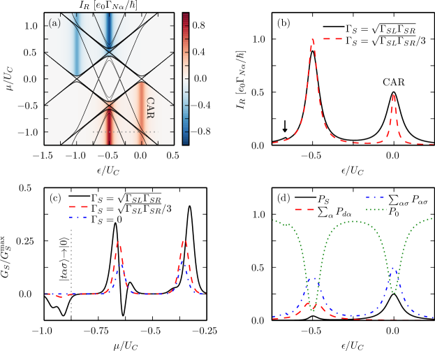
Figure 2: (a) Current $I_{R}$ through the right lead as a function of the dots’ level positions $\epsilon\equiv\epsilon_{L}=\epsilon_{R}$, and the chemical potential $\mu\equiv\mu_{L}=\mu_{R}$, where the solid lines indicate the condition under which the chemical potential is equal to the Andreev addition energies. Parameters are $\Gamma_{S}=\Gamma_{S\alpha}=7.5\ 10^{-2}U_{C}$, $t=U=0$, and $k_{B}T=2.5\ 10^{-3}U_{C}$, and $\Gamma_{N\alpha}=2.5\ 10^{-4}U_{C}$. (b) Current $I_{R}$ as a function of the dots’ level positions $\epsilon\equiv\epsilon_{L}=\epsilon_{R}$ at constant $\mu=-U_{C}$ for intermediate nonlocal coupling $\Gamma_{S}=\Gamma_{S\alpha}/3$ (dashed line), and maximal nonlocal coupling $\Gamma_{S}=\Gamma_{S\alpha}$ (solid line). The value $\mu=-U_{C}$ is indicated in panel (a) by a dotted line. The arrow indicates the transition $|t\alpha\sigma\rangle\to|0\rangle$. (c) Differential conductance $G_{S}\equiv dI_{S}/dV$ at constant $\epsilon=-0.625U_{C}$ for $\Gamma_{S\alpha}=10k_{B}T=0.125U_{C}$, normalized by its maximum $G_{S}^{\textrm{max}}$ at constant $\epsilon=-U_{C}/2$. (d) Occupation probabilities as a function of the level position for $\mu=-U_{C}$ and maximal nonlocal coupling $\Gamma_{S}=\Gamma_{S\alpha}$.

From the cumulant generating function, $Z(\bm{\chi},\bm{\mu})=\lim_{t\to\infty}\frac{\partial}{\partial t}\ln\operatorname{tr}P({\bm{\chi},\bm{\mu}})$, we can obtain the stationary current $I_{\alpha}=\partial Z/\partial i\chi_{\alpha}|_{{\bm{\chi}}={\bm{0}}}$ in the normal lead $\alpha=L,R$ and the corresponding differential conductance $G_{\alpha,\beta}=-\partial^{2}Z/\partial i\chi_{\alpha}\partial\mu_{\beta}|_{{\bm{\chi}}={\bm{0}}}$. Both the currentFlindt et al. (2008, 2010) and the conductanceHussein and Kohler (2014) can be calculated in the usual iterative scheme.

III transport in absence of interdot tunneling

In this section, we give an overview of how the local and nonlocal proximization affects quantum transport in absence of interdot tunneling. In particular, we start discussing the two limits $\Gamma_{S\alpha}\gg U$ and $U\gtrsim\Gamma_{S\alpha}$. Both limits feature a resonant current originating from the CAR process. The former case of weak interdot Coulomb energy is typically realized in experiments.Schindele et al. (2012) The limit of strong interdot Coulomb energy additionally permits to study resonant currents which are entirely characterized by LAR. Throughout this work, we consider identical quantum dots, i.e. $U_{L}=U_{R}\equiv U_{C}$, $\Gamma_{SL}=\Gamma_{SR}\equiv\Gamma_{S\alpha}$, and $\Gamma_{N}\equiv\Gamma_{NL}=\Gamma_{NR}$. We limit to the case of equal orbital levels in the two quantum dots, $\epsilon\equiv\epsilon_{L}{=}\epsilon_{R}$, and equal chemical potentials $\mu\equiv\mu_{L}{=}\mu_{R}$.

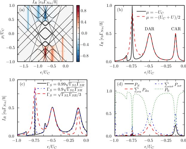
Figure 3: (a) Current $I_{R}$ through the right lead as a function of the gate voltage $\epsilon\equiv\epsilon_{L}=\epsilon_{R}$, and the chemical potential $\mu\equiv\mu_{L}=\mu_{R}$ for finite $U=0.25\ U_{C}$ and $\Gamma_{S}=\Gamma_{S\alpha}/3$. Other parameters are as in Fig. 2. (b) Corresponding slices at constant $\mu=-(U_{C}+U)/2$ (dashed line), and $\mu=-U_{C}$ (solid line). The slice at $\mu=-(U_{C}+U)/2$ is indicated in panel (a) by a dotted line. (c) Current $I_{R}$ at constant $\mu=-(U_{C}+U)/2$ for various values of $\Gamma_{S}$. (d) Corresponding population probabilities as a function of the gate voltage $\epsilon$ at fixed $\mu=-U_{C}$.

III.1 Weak interdot Coulomb energy, $U\approx 0$

In Fig. 2(a), we show a density plot of the current in the right lead $I_{R}(\epsilon,\mu)$ as a function of the dots’ level $\epsilon$, which can be tuned by gate voltages, and the chemical potential $\mu$ of the normal leads. We notice that the current in the normal leads obeys the symmetry $I_{\alpha}(\epsilon,\mu)=-I_{\alpha}(2\epsilon_{0}-\epsilon,-\mu)$ with $\epsilon_{0}=-(U_{C}/2+U)$. This symmetry is due the particle-hole (PH) symmetry of the Hamiltonian Eq. (4) in the absence of interdot tunneling.

We focus on the situation $\mu<0$ which corresponds to the transport of Cooper pairs from the superconductor to the double-dot system. Two resonances can be seen in Fig. 2(a): one at $\epsilon=\epsilon_{\textrm{CAR}}=-U/2$ that is caused only by CAR and another at $\epsilon=\epsilon_{0}$ which originates from both CAR and LAR. The current is asymmetrical with respect to the chemical potentials $\mu$. The bias asymmetry of the CAR peak is due to the triplet blockade: for $\mu>0$ tunneling of electrons from the leads can bring the double-dot in a triplet state whose spin symmetry is incompatible with the BCS superconductor, hence blocking the CAR.Eldridge et al. (2010)

Along the level position axis, the CAR resonance is centered at $\epsilon_{\textrm{CAR}}$ and its broadening is $\sqrt{2}\Gamma_{S}$. This can be seen in panel (b) of Fig. (2), which shows the current at constant $\mu=-U_{C}$ for two different values of the nonlocal coupling: $\Gamma_{S}=\sqrt{\Gamma_{SL}\Gamma_{SR}}/3$ (dashed line) and $\Gamma_{S}=\sqrt{\Gamma_{SL}\Gamma_{SR}}$ (solid line). The CAR broadening is proportional to the nonlocal coupling $\Gamma_{S}$ but its height does not depend on it. The CAR resonance instead follows the singlet population, i.e. $\hbar I_{R}^{\textrm{CAR}}/e_{0}\Gamma_{NR}\approx 2P_{S}$, as can be seen in panel (d). The states involved in the CAR process are $|0\rangle$, $|\alpha\sigma\rangle$, $|S\rangle$ and in fact one only observes the corresponding populations, $P_{0}+\sum_{\alpha\sigma}P_{\alpha\sigma}+P_{S}\approx 1$. On the contrary, the resonance at $\epsilon=-U_{C}/2$ is mainly due to the LAR, but involves also CAR as indicated by the non-vanishing singlet population at the LAR resonance [see panel (d)].

We will discuss now that strong superconducting coupling may also generate negative differential conductance (NDC) when single electron tunneling events with the normal leads are accompanied by a simultaneous exchange of a Cooper-pair. For instance if one of the dots is doubly occupied, while the other is singly occupied, it can occur that an electron leaves the system through a normal-metal lead and the two remaining electrons tunnel (locally or nonlocally) to the superconductor. If the process is energetically admissible the total current is reduced instead of increased by the opening of the new resonance and NDC is observed.

This is indeed observed in panel (c) of Fig. 2 having defined the conductance as $G_{S}\equiv dI_{S}/dV$. We show $G_{S}$ as function of the chemical potential, for a fixed level position $\epsilon=\epsilon_{0}-0.125U_{C}$. The differential conductance becomes negative around $\mu\approx 3\epsilon+U_{C}$ (leftmost peak). This extra resonance corresponds energetically to the transition from the triply occupied states to the empty state, $|t\alpha\sigma\rangle\to|0\rangle$, where two electrons tunnel in the superconductor and the remaining electron tunnels in one of the normal leads. This involves only the exchange of a nonlocal Cooper pair and is no longer present in the absence of nonlocal coupling [dot-dashed line in panel (c) of Fig. 2]. In order to increase the visibility of the NDC we have chosen a stronger nonlocal coupling $\Gamma_{S}$ (by increasing $\Gamma_{S\alpha}$) to obtain a higher peak value and slightly higher temperatures to increase the linewidth of this resonance in comparison to other figures.

III.2 Finite interdot Coulomb energy, $U\gtrsim\Gamma_{S\alpha}$

For finite interdot Coulomb energy the LAR dominated resonance in Fig. 2(a) splits into two resonances at gate voltages $\epsilon_{\textrm{LAR}}=-U_{C}/2$ and $\epsilon_{0}=\epsilon_{\textrm{LAR}}-U$ as can be seen in panel (a) of Fig. 3. The former current resonance is purely affected by LAR involving the states $|0\rangle$, $|\alpha\sigma\rangle$, $|d\alpha\rangle$. In fact, in panel 3(d) one observes that only the corresponding populations are non vanishing, i.e. $P_{0}+\sum_{\alpha\sigma}P_{\alpha\sigma}+\sum_{\alpha}P_{d\alpha}\approx 1$ and that the current is proportional the population of the doubly occupied state, $\hbar I_{R}^{\textrm{LAR}}/e_{0}\Gamma_{NR}\approx 4P_{dR}$. We still observe the asymmetry of the nonlocal-current resonances in the chemical potential due to the triplet blockade. Additionally, one notices an asymmetry of the LAR resonances, which can be explained partly by the triplet blockade mechanism and partly by energy considerations.

The central resonance at $\epsilon_{0}=\epsilon_{\textrm{LAR}}-U$ is affected both by the LAR and the CAR processes. For an intermediate value of the chemical potentials [see dashed line in panel (b) of Fig. (3)] its width is roughly proportional to $\sqrt{\Gamma_{SL}\Gamma_{SR}}-\Gamma_{S}$ and vanishes if $\Gamma_{S}$ becomes maximal. In panel (c) we demonstrate the effect of the nonlocal Cooper-pair tunneling on the current resonances, for an intermediate value of the chemical potentials and for different values of the nonlocal coupling $\Gamma_{S}$. The dashed line corresponds to the dashed line in panel (b). When $\Gamma_{S}$ approaches its maximum, the width of the central resonance (left peak) tends to zero while its height remains unaffected. We suspect that the behavior of the width of this central resonance is due to the mutual exclusion of the local Cooper-pair tunneling process and the nonlocal one, and originates from a destructive interference of the two channels (see also later). On the contrary, if both processes were independent, the linewidth would be the sum of both contributions. In conclusion this regime of finite interdot Coulomb energy can be helpful to assess the strength of the nonlocal coupling $\Gamma_{S}$ in comparison to the local terms.

IV Influence of interdot tunneling and spin-orbit interaction

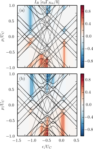
Figure 4: (a) Current $I_{R}$ through the right lead as a function of the gate voltage $\epsilon=\epsilon_{L}=\epsilon_{R}$ and chemical potential $\mu=\mu_{R}=\mu_{L}$ for finite interdot tunneling with $t=0.4\>U_{C}$ and the SO angle $\phi=0$. Other parameters are $U=0$, $\Gamma_{S}=\Gamma_{S\alpha}=7.5\ 10^{-2}U_{C}$, $\Gamma_{N\alpha}=2.5\ 10^{-4}U_{C}$ and $k_{B}T=2.5\ 10^{-3}U_{C}$. (b) Current $I_{R}$ for the same parameters as in panel (a) but for finite SO interaction with an SO angle of $\phi=\pm\pi/2$.

In this section, we consider the effect of finite interdot tunneling and SO interaction on the current $I_{R}$. For the sake of simplicity we consider in the following only the case $\phi=0$ (no SO coupling) and $\phi=\pm\pi/2$ (finite SO coupling with $k_{SO}l=\pi/2$). Let us first focus on the general behavior of the current as a function of the level position and chemical potential as shown in the density plots of Fig. 4. For simplicity we consider the case without interdot Coulomb energy, $U=0$, which describes well the situation of $\Gamma_{S\alpha}\gg U$. Finally, in order to see stronger signatures of the interdot tunneling term we generally consider $U_{C}\gg t\gg\Gamma_{S},\Gamma_{S\alpha}$.

In the top panel we show the case of finite interdot tunneling in the absence of SO coupling, i.e. $\phi=0$, which can be directly compared with the density plot of Fig. 2(a) where the interdot tunneling was absent. One immediately sees that the Andreev resonant lines (black solid lines) are generally split in comparison to the case without interdot tunneling, giving rise to an even richer Andreev-bound-state spectrum. The most general observation is that the PH symmetry of the transport properties, as discussed in section III, is broken, i.e. $I_{\alpha}(\epsilon,\mu)\neq-I_{\alpha}(2\epsilon_{0}-\epsilon,-\mu)$ with $\epsilon_{0}=-(U_{C}/2+U)$. The breaking of the PH symmetry in transport is observed if both the quantities $\Gamma_{S},\Gamma_{S\alpha}\neq 0$. On the other hand if one of these quantities vanishes the PH symmetry is restored. We discuss PH-symmetry breaking in more detail in Sec. IV.1.

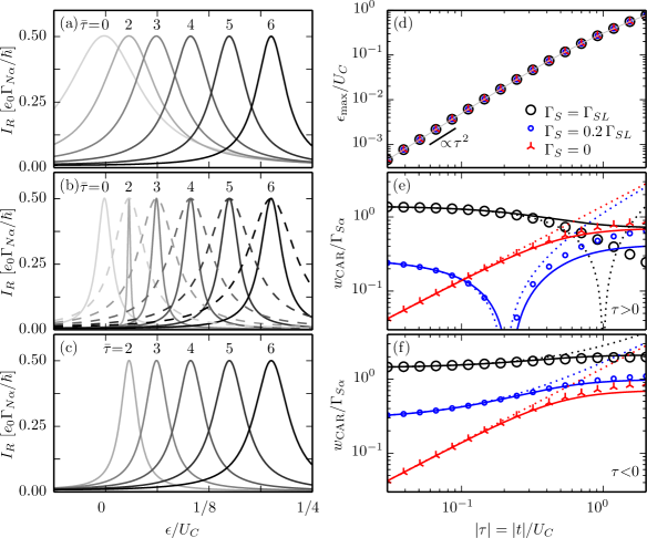
Figure 5: (a)-(c) Current $I_{R}$ in the CAR resonance as a function of the gate voltage for different values of the tunneling amplitude, $\bar{\tau}=8|t|/U_{C}$, for the nonlocal term $\Gamma_{S}/\sqrt{\Gamma_{SR}\Gamma_{SL}}=1$ [panel (a)], $1/3$ [panel (b)], $0$ [panel (c)] and other parameters as in Fig. 2. The solid lines correspond to $t/U_{C}>0$ while the dashed lines in panel (b) correspond to $t/U_{C}<0$. (d) Gate position at the maximum of the CAR resonance, $\epsilon_{\textrm{CAR}}$, as a function of the scaling variable $\tau=t/U_{C}$ for the different values of the nonlocal term considered in the panels (a)-(c). (e)-(f) CAR resonance linewidth $w_{\mathrm{CAR}}$ as a function of the scaling variable $|\tau|$ [$\tau>0$ for (e) and $\tau<0$ for (f)] for the different values of the nonlocal term considered in the panels (a)-(c); the solid and dotted lines in panel (d)-(f) are the theoretical predictions in the simplified model discussed in the main text.

In the bottom panel of Figure 4, instead, we show how the current is affected by tunneling in the presence of the SO coupling, for the case $\phi=\pm\pi/2$. We see that in this case the PH symmetry is again restored for any value of of $\Gamma_{S}$ and $\Gamma_{S\alpha}$. Note that the Andreev addition energies spectrum becomes also quite intricate and it is not so useful to enter in the details of the behavior of any resonant line. In general one can see that in comparison to the top panel crossings and avoided crossings occur between different pairs of Andreev levels. This is a natural consequence of the different symmetry of the tunnel coupling between the two dots in the two cases. Finally, for $\Gamma_{S},\Gamma_{S\alpha}\neq 0$, the CAR peaks are split along the level-position axis and an extra resonance appears. We will discuss in detail the nature of this extra resonance in Sec. IV.2

IV.1 Interdot tunneling and breaking of PH

To investigate the PH symmetry breaking, we apply the PH transformation $d_{\alpha\sigma}\to d^{\dagger}_{\alpha-\sigma}$ to Eq. (4). It is easy to check that indeed this transformation leaves obviously unaffected the local and nonlocal pairing terms but is equivalent to a change of sign of the interdot tunneling term, i.e. $t\to-t$. Therefore, the symmetry obeyed by the current is $I_{\alpha}(\epsilon,\mu,t)\to-I_{\alpha}(2\epsilon_{0}-\epsilon,-\mu,-t)$ which we have numerically verified. Notice that the sign of $t$ in the tunneling Hamiltonian cannot be gauged away only if both the local and nonlocal pairing terms are present in Eq. (4). Finally, we notice that for $|\phi|=\pi/2$ the sign of $t$ is unessential due to Kramer’s degeneracy and therefore the PH symmetry is restored in this special case.

It remains the question why the sign and more generally a phase of $t$ is detectable in the transport properties of the system. This is essentially due to the interference between two paths connecting the empty state with the singlet state. One path is the nonlocal Andreev tunneling with rate $\Gamma_{S}$ while the other is the process where a Cooper-pair virtually tunnels into one of the dots bringing it in the doubly occupied state and subsequently this state is converted into a singlet state by interdot tunneling. The interference between the two paths is clearly affected by the phase (not only the sign) of $t$. In order to observe this interference effect the doubly occupied state of a single dot needs to be accessible. We have verified that, for $U_{C}\to\infty$, an overall phase of $t$ does not affect the transport properties of the system.

IV.2 Weak interdot Coulomb energy, $\Gamma_{S\alpha}\gg U$

We focus on the effect of the interdot tunneling on the CAR resonance. In Fig. 5 (a)-(c) we show the evolution of the CAR current peak for different values of $|t|$ for $\phi=0$. For increasing strength of the interdot tunneling, the position of the CAR resonance shifts to the right and at the same time the resonance linewidth changes. The peak shift is $\delta\epsilon_{\textrm{CAR}}/U_{C}\approx(1/2)(t/U_{C})^{2}$ for $t\ll U_{C}$. This is shown in the panel Fig. 5(d) where the position of the CAR peak maximum $\epsilon_{\textrm{max}}$ is plotted as a function of $\tau=t/U_{C}$. For different values of the nonlocal coupling $\Gamma_{S}$ [different point styles in panel (d)] the peak position follows the same universal function of $\tau$ (solid line). Instead the linewidths, shown in Fig. 5(e)-(f), exhibit quite different behaviors depending on the value of $\Gamma_{S}$, the strength of $t$ and also its sign.

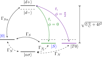
Figure 6: Effective level structure at the CAR resonance. Finite interdot tunneling ($\phi=0$) leads to a level repulsion between the symmetric state $|d+\rangle=(|dR\rangle+|dL\rangle)/\sqrt{2}$ and the singlet state $|S\rangle$, see Eq. (9). SO interaction ($\phi=\pi/2$) leads instead to a level repulsion between the unpolarized triplet state $|T0\rangle$ and the symmetric state $|d+\rangle$. The symmetric state, virtually occupied by local Cooper-pair tunneling, plays the role of a dark state.

These observations can be explained by making use of a reduced Hilbert space which describes well the system in the vicinity of the CAR resonance. This simplified model is sketched in Fig. 6. The relevant states for the CAR resonance are the empty state $|0\rangle$, the singlet state $|S\rangle$, and the singly occupied states $|\alpha\sigma\rangle$. The states in the even sector $|0\rangle$ and $|S\rangle$ are connected via the nonlocal term $\Gamma_{S}$, and they are connected to the singly occupied states $|\alpha\sigma\rangle$ via the tunneling rate to the normal lead, $\Gamma_{N}$. In the absence of interdot tunneling the CAR resonance linewidth is only determined by the nonlocal term $\Gamma_{S}$, see section III. However, for finite intradot Coulomb energy in the presence of local terms $\Gamma_{S\alpha}$ and strong interdot tunneling $t$ (with $\phi=0$), we need to consider also another possibility: when the quantum-dots are in the empty state a Cooper pair can be virtually transferred by means of the local term $\Gamma_{S\alpha}$ in the doubly occupied state $|d\alpha\rangle$ which is converted to the singlet state via the interdot tunneling. One can see in Eq. (12) that the tunneling amplitude $(t/\sqrt{2})\cos(\phi)$ couples the $|d\alpha\rangle$ states with the singlet state $|S\rangle$. We will quantitatively show that the interference of this alternative channel with the standard nonlocal process fully determines the observed behavior of the CAR peak.

When $\Gamma_{S}\ll t$, the peak shift can be understood in terms of the level repulsion of the singlet state with the doubly occupied state. We first note that the interdot coupling removes the degeneracy of the double occupancies and yields the states $|d\pm\rangle=(|dR\rangle\pm|dL\rangle)/\sqrt{2}$. Only the symmetric state $|d+\rangle$ is affected by the level repulsion with $|S\rangle$. In this model the hybridized states $|\pm\rangle\approx\alpha|S\rangle\pm\beta|d+\rangle$ with $\alpha$, $\beta$ c-numbers have the energies

$$\frac{\epsilon_{\pm}}{U_{C}}=\frac{1+4\epsilon/U_{C}\pm\sqrt{1+4\tau^{2}}}{2}\>,$$ (9)

where $\tau=t/U_{C}$. The position of the CAR resonance is the solution of equation $\epsilon_{-}(\epsilon_{CAR})=0$, the resonance condition between $|-\rangle$ and the empty state $|0\rangle$. The peak position is $\epsilon_{\textrm{CAR}}=(\sqrt{1+4\tau^{2}}-1)U_{C}/4$, which fits well the shifting of the peak position [see solid line in Fig. 5(d)]. In the limit $U_{C}\to\infty$ ($\tau\to 0$) the doubly occupied states are unaccessible, even virtually, and the transport becomes independent of the interdot tunneling.

Finite interdot tunneling also modifies the linewidth of the CAR peak as can be seen in Fig. 5(a)-(c) and more clearly in Fig. 5(e)-(f) where we show the linewidth $w_{\textrm{CAR}}$ of the CAR resonance. For $\Gamma_{S}=\sqrt{\Gamma_{SL}\Gamma_{SR}}$ (black circles) the width is roughly proportional to the nonlocal coupling while for $\Gamma_{S}=0$ (red triangles) it increases with $\tau$. Intriguingly, for an intermediate value of $\Gamma_{S}$ (blue small circles) and $\tau>0$, the linewidth almost vanishes for a specific value of $\tau$ [see Fig. 5(e)]. This behavior is not seen for $\tau<0$ [see Fig. 5(f)].

We can explain these results by making use again of the simplified model shown in Fig. 6. In the absence of the interdot tunneling the linewidth of the CAR peak is only determined by the strength of the coupling between the empty state $|0\rangle$ and the singlet state $|S\rangle$. Essentially, it is given by the off-diagonal matrix element $w_{\textrm{CAR}}\approx 2|\langle 0|H_{S}|S\rangle|=\sqrt{2}\Gamma_{S}$. Any additional process that contributes to that coupling between $|0\rangle$ and $|S\rangle$, also through a virtual high energy state, will affect the linewidth. This correction may be obtained considering the effective Hamiltonian $H_{S}=H_{0}+V$, which represents the model shown in Fig. 6, with $H_{0}=\sum_{i}E_{i}|i\rangle\langle i|-(\Gamma_{S}/\sqrt{2})(|0\rangle\langle S|+|S\rangle\langle 0|)$ for $i=0,S,d+,d-$ and the perturbation $V=\big{[}t|d+\rangle\langle S|-(\Gamma_{S\alpha}/\sqrt{2})|d+\rangle\langle 0|+\mathrm{H.c.}\big{]}$. Calculating the off-diagonal matrix element up second order in the perturbation, $\mathcal{O}(V^{3})$, yieldsBerestetskii et al. (1982)

$$\langle 0|H_{S}|S\rangle=\langle 0|H_{0}|S\rangle+\frac{\langle 0|V|d+\rangle\langle d+|V|S\rangle}{E^{(0)}_{S}-E^{(0)}_{d+}}$$ (10)

with $E^{(0)}_{S}-E^{(0)}_{d+}=-U_{C}$. We find for the linewidth $w_{\textrm{CAR}}\approx\sqrt{2}|\Gamma_{S}-\Gamma_{S\alpha}\tau|$. This estimation of the linewidth is indicated by dotted lines in Fig. 5(e)-(f). It turns out to be a quite good approximation for $\tau\lll 1$ but it worsens for increasing $\Gamma_{S}$ (see for example the black case $\Gamma_{S}=\sqrt{\Gamma_{SL}\Gamma_{SR}}$). A better approximation, however, is obtained by the substitution $E^{(0)}_{S}-E^{(0)}_{d+}\to\epsilon_{-}-\epsilon_{+}=-U_{C}\sqrt{1+4\tau^{2}}$ which includes the energy renormalization effects induced by the level repulsion discussed before. Therefore, the linewidth can be approximated by

$$w_{\textrm{CAR}}\approx\sqrt{2}\Bigg{|}\Gamma_{S}-\frac{\Gamma_{S\alpha}\tau}{\sqrt{1+4\tau^{2}}}\Bigg{|}$$ (11)

which fits (solid lines) well the numerical results based on the full Hamiltonian, see Fig. 5(e)-(f). Interestingly Eq.  (11) explains also why for positive (negative) sign of $t$ the linewidth can decrease (increase) due to destructive (constructive) interference. This is seen comparing the results for $\Gamma_{S}=0.2\sqrt{\Gamma_{SL}\Gamma_{SR}}$ in panel (e) and (f) of Fig. 5. Finally, one intriguing consequence of the virtual-state process involving the state $|d+\rangle$ is that it generates nonlocal entangled electrons even in the absence of a direct nonlocal coupling.

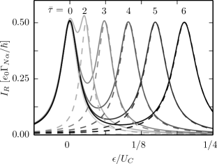
Figure 7: Current $I_{R}$ in the CAR resonance as a function of the gate voltage for different values of the tunneling amplitude, $\bar{\tau}=8|t|/U_{C}$, $\phi=\pm\pi/2$ for $\Gamma_{S}=\Gamma_{S\alpha}/3$ (solid line) and $\Gamma_{S}=0$ (dashed line) keeping fixed the $U_{C}$. Other parameters as in Fig. 5.

We now turn our attention to the case with the SO coupling and $\phi=\pm\pi/2$. We see in panel (b) of Fig. 4 that the CAR resonance splits into two lines, one at $\epsilon\approx 0$ and the other shifted towards higher values of $\epsilon$. In Fig. 7 we show the behavior of the CAR peak with increasing values of $t$ for constant values of $U_{C}$ and $\Gamma_{S}$. First we notice that for $\Gamma_{S}=0$ (dashed lines) the CAR peak does not split but it shifts to the right for increasing values of $\tau$ and no resonance is present at $\epsilon\approx 0$. Instead, for $\Gamma_{S}\neq 0$, the resonance splits into two resonances, one fixed at $\epsilon\approx 0$ and the other right-shifted with $\delta\epsilon_{\textrm{rs}}/U_{C}\approx(1/2)(t/U_{C})^{2}$. This demonstrates the connection with the nonlocal term $\Gamma_{S}$ of the CAR peak at $\epsilon\approx 0$.

We numerically observed that the current of the right-shifted peak follows the population of the unpolarized triplet state, $\hbar I_{R}^{\textrm{rs}}/e_{0}\Gamma_{NR}\approx 2P_{T0}$. These observations suggest that a resonant mechanism involving the virtual occupation of the $|d+\rangle$ is established with the unpolarized triplet state $|T0\rangle$, as depicted schematically in Fig. 6. This mechanism is analogous to the one induced by the nonlocal singlet proximity in the case of interdot coupling where $\phi=0$. We refer to this resonance as triplet CAR resonance, since it generates nonlocal entanglement with triplet symmetry. The position and linewidth of this right-shifted resonance are described by Eq. (9) and Eq. (11) setting $\Gamma_{S}=0$, respectively. This is a consequence of the fact that a $s$-wave superconductor cannot induce directly triplet correlations. This shows how the presence of SO coupling can nevertheless induce nonlocal triplet superconducting correlations even when the only superconducting lead has $s$-wave pairing symmetry.Shekhter et al. (2016); Yu and Wu (2016)

V Conclusions

We have presented a comprehensive study of a Cooper-pair splitter based on a double-quantum dot. Employing a master-equation description, in the framework of FCS, we have calculated the current injected into the normal leads. We have considered a finite intra-dot interaction which allows the local transfer of Cooper-pairs from the superconductor to an individual quantum dot. We have studied the signatures of local and nonlocal Andreev reflection in the current injected in the normal leads. The interdot Coulomb interaction separates the local and nonlocal resonances. The effect of interdot tunneling both with and without SO coupling has been considered, too. In particular, we find that the interdot tunneling can induce nonlocal entanglement starting from local Andreev reflection. Furthermore, a process including the virtual doubly-occupied states of the individual dots leads to modifications of the position and linewidth of the current resonances. For the case with SO coupling, we find that a nonlocal triplet pair amplitude can be generated in the system. This mechanism involving the virtual occupation of the doubly occupied states is active only for finite intradot Coulomb interaction.

Appendix A Matrix representation of the system Hamiltonian

In this section we provide the decomposition of the system Hamiltonian $H_{S}=H_{S}^{\textrm{even}}\oplus H_{S}^{\textrm{odd}}$ into sectors with even and odd parity. We assume the single particle level spacing in the quantum dot to be large compared to $U$, $U_{\alpha}$ and the interdot tunneling $t$, so the total dimension of the system Hilbert space reduces to $16$ states ($8$ even $+$ $8$ odd). Here, we express Eq. (4) in the even sector basis $\{|0\rangle,|S\rangle,|dL\rangle,|dR\rangle,|dd\rangle,|T0\rangle,|T\!\!\uparrow\rangle,|T\!\!\downarrow\rangle\}$ stated in table 1. The Hamiltonian for the even charge sector reads

$$H_{S}^{\textrm{even}}=$$

$${\small\begin{pmatrix}0&-\frac{1}{\sqrt{2}}\Gamma_{S}&-\frac{1}{2}\Gamma_{SL}&-\frac{1}{2}\Gamma_{SR}&0&0&0&0\\ -\frac{1}{\sqrt{2}}\Gamma_{S}&\epsilon_{L}+\epsilon_{R}+U&\frac{t}{\sqrt{2}}\cos(\phi)&\frac{t}{\sqrt{2}}\cos(\phi)&+\frac{1}{\sqrt{2}}\Gamma_{S}&0&0&0\\ -\frac{1}{2}\Gamma_{SL}&\frac{t}{\sqrt{2}}\cos(\phi)&2\epsilon_{L}+U_{L}&0&-\frac{1}{2}\Gamma_{SR}&i\frac{t}{\sqrt{2}}\sin(\phi)&0&0\\ -\frac{1}{2}\Gamma_{SR}&\frac{t}{\sqrt{2}}\cos(\phi)&0&2\epsilon_{R}+U_{R}&-\frac{1}{2}\Gamma_{SL}&i\frac{t}{\sqrt{2}}\sin(\phi)&0&0\\ 0&+\frac{1}{\sqrt{2}}\Gamma_{S}&-\frac{1}{2}\Gamma_{SR}&-\frac{1}{2}\Gamma_{SL}&2(\epsilon_{R}+\epsilon_{L})+U_{R}+U_{L}+4U&0&0&0\\ 0&0&-i\frac{t}{\sqrt{2}}\sin(\phi)&-i\frac{t}{\sqrt{2}}\sin(\phi)&0&\epsilon_{L}+\epsilon_{R}+U&0&0\\ 0&0&0&0&0&0&\epsilon_{L}+\epsilon_{R}+U&0\\ 0&0&0&0&0&0&0&\epsilon_{L}+\epsilon_{R}+U\\ \end{pmatrix}}.$$ (12)

Note that the interdot tunneling preserves the spin of the tunneling electrons (being time reversal invariant) and the total parity of the DQD. In absence of the SO interaction, $\phi=0$, all triplet states $|Ti\rangle$ are completely decoupled from the other even parity states. When $\phi\neq\pi k$, where $k$ integer, the unpolarized triplet state $|T0\rangle$ couples with the doubly occupied states $|d\alpha\rangle$. The Hamiltonian for the odd charge sector, in the basis $\{|R\!\!\uparrow\rangle,|R\!\!\downarrow\rangle,|L\!\!\uparrow\rangle,|L\!\!\downarrow\rangle,|tR\!\!\uparrow\rangle,|tR\!\!\downarrow\rangle,|tL\!\!\uparrow\rangle,\\ |tL\!\!\downarrow\rangle\}$, is given by

$$H_{S}^{\text{odd}}=\begin{pmatrix}\epsilon_{R}&0&\frac{t}{2}e^{-i\phi}&0&-\frac{1}{2}\Gamma_{SL}&0&+\frac{1}{2}\Gamma_{S}&0\\ 0&\epsilon_{R}&0&\frac{t}{2}e^{+i\phi}&0&-\frac{1}{2}\Gamma_{SL}&0&+\frac{1}{2}\Gamma_{S}\\ \frac{t}{2}e^{+i\phi}&0&\epsilon_{L}&0&+\frac{1}{2}\Gamma_{S}&0&-\frac{1}{2}\Gamma_{SR}&0\\ 0&\frac{t}{2}e^{-i\phi}&0&\epsilon_{L}&0&+\frac{1}{2}\Gamma_{S}&0&-\frac{1}{2}\Gamma_{SR}\\ -\frac{1}{2}\Gamma_{SL}&0&+\frac{1}{2}\Gamma_{S}&0&E_{tR\uparrow}&0&-\frac{t}{2}e^{-i\phi}&0\\ 0&-\frac{1}{2}\Gamma_{SL}&0&+\frac{1}{2}\Gamma_{S}&0&E_{tR\downarrow}&0&-\frac{t}{2}e^{+i\phi}\\ +\frac{1}{2}\Gamma_{S}&0&-\frac{1}{2}\Gamma_{SR}&0&-\frac{t}{2}e^{+i\phi}&0&E_{tL\uparrow}&0\\ 0&+\frac{1}{2}\Gamma_{S}&0&-\frac{1}{2}\Gamma_{SR}&0&-\frac{t}{2}e^{-i\phi}&0&E_{tL\downarrow}\\ \end{pmatrix},$$ (13)

where $E_{t\alpha\sigma}=2\epsilon_{\bar{\alpha}}+U_{\bar{\alpha}}+\epsilon_{\alpha}+2U$ with $\alpha=R,L$ ($\bar{\alpha}=L,R$) and $\sigma=\uparrow,\downarrow$.

References

- Monroe (2002) C. Monroe, Nature 416, 238 (2002).
- Martinis (2009) J. Martinis, Quantum Inf. Process. 8, 81 (2009).
- Ladd et al. (2010) T. D. Ladd, F. Jelezko, R. Laflamme, Y. Nakamura, C. Monroe, and J. L. O’Brien, Nature 464, 45 (2010).
- Lo et al. (2014) H.-K. Lo, M. Curty, and K. Tamaki, Nature Photon. 8, 595 (2014).
- Linder and Robinson (2015) J. Linder and J. W. A. Robinson, Nature Phys. 11, 307 (2015).
- Yoshimi et al. (2015) R. Yoshimi, A. Tsukazaki, Y. Kozuka, J. Falson, K. Takahashi, J. Checkelsky, N. Nagaosa, M. Kawasaki, and Y. Tokura, Nature Commun. 6, 6627 (2015).
- Qi and Zhang (2011) X.-L. Qi and S.-C. Zhang, Rev. Mod. Phys. 83, 1057 (2011).
- Kitaev (2001) A. Kitaev, Phys. Usp. 44, 131 (2001).
- Nayak et al. (2008) C. Nayak, S. H. Simon, A. Stern, M. Freedman, and S. Das Sarma, Rev. Mod. Phys. 80, 1083 (2008).
- Alicea (2012) J. Alicea, Rep. Prog. Phys. 75, 076501 (2012).
- Romeo et al. (2012) L. Romeo, S. Roddaro, A. Pitanti, D. Ercolani, L. Sorba, and F. Beltram, Nano Lett. 12, 4490 (2012).
- Rossella et al. (2014) F. Rossella, A. Bertoni, D. Ercolani, M. Rontani, L. Sorba, F. Beltram, and S. Roddaro, Nature Nano 9, 997 (2014).
- Giazotto et al. (2011) F. Giazotto, P. Spathis, S. Roddaro, S. Biswas, F. Taddei, M. Governale, and L. Sorba, Nature. Phys. 7, 857 (2011).
- Roddaro et al. (2011) S. Roddaro, A. Pescaglini, D. Ercolani, L. Sorba, F. Giazotto, and F. Beltram, Nano Res. 4, 259 (2011).
- Spathis et al. (2011) P. Spathis, S. Biswas, S. Roddaro, L. Sorba, F. Giazotto, and F. Beltram, Nanotechnology 22, 105201 (2011).
- Lee et al. (2014) E. J. H. Lee, X. Jiang, M. Houzet, R. Aguado, C. M. Lieber, and S. De Franceschi, Nature Nano 9, 79 (2014).
- Yokoyama et al. (2014) T. Yokoyama, M. Eto, and Y. V. Nazarov, Phys. Rev. B 89, 195407 (2014).
- Mironov et al. (2015) S. V. Mironov, A. S. Mel’nikov, and A. I. Buzdin, Phys. Rev. Lett. 114, 227001 (2015).
- Žonda et al. (2015) M. Žonda, V. Pokornỳ, V. Janiš, and T. Novotnỳ, Sci. Rep. 5, 8821 (2015).
- Marra et al. (2016) P. Marra, R. Citro, and A. Braggio, Phys. Rev. B 93, 220507 (2016).
- Shekhter et al. (2016) R. I. Shekhter, O. Entin-Wohlman, M. Jonson, and A. Aharony, Phys. Rev. Lett. 116, 217001 (2016).
- Yu and Wu (2016) T. Yu and M. W. Wu, Phys. Rev. B 93, 195308 (2016).
- Bouchiat et al. (2003) V. Bouchiat, N. Chtchelkatchev, D. Feinberg, G. B. Lesovik, T. Martin, and J. Torrès, Nanotechnology 14, 77 (2003).
- Russo et al. (2005) S. Russo, M. Kroug, T. M. Klapwijk, and A. F. Morpurgo, Phys. Rev. Lett. 95, 027002 (2005).
- Schindele et al. (2012) J. Schindele, A. Baumgartner, and C. Schönenberger, Phys. Rev. Lett. 109, 157002 (2012).
- Fülöp et al. (2014) G. Fülöp, S. d’Hollosy, A. Baumgartner, P. Makk, V. A. Guzenko, M. H. Madsen, J. Nygård, C. Schönenberger, and S. Csonka, Phys. Rev. B 90, 235412 (2014).
- Das et al. (2012) A. Das, Y. Ronen, M. Heiblum, D. Mahalu, A. V. Kretinin, and H. Shtrikman, Nature Commun. 3, 1165 (2012).
- Schindele et al. (2014) J. Schindele, A. Baumgartner, R. Maurand, M. Weiss, and C. Schönenberger, Phys. Rev. B 89, 045422 (2014).
- He et al. (2014) J. J. He, J. Wu, T.-P. Choy, X.-J. Liu, Y. Tanaka, and K. T. Law, Nature Commun. 5, 3232 (2014).
- Ishizaka et al. (1995) S. Ishizaka, J. Sone, and T. Ando, Phys. Rev. B 52, 8358 (1995).
- Deacon et al. (2015) R. S. Deacon, A. Oiwa, J. Sailer, S. Baba, Y. Kanai, K. Shibata, K. Hirakawa, and S. Tarucha, Nature Commun. 6, 7446 (2015).
- Recher et al. (2001) P. Recher, E. V. Sukhorukov, and D. Loss, Phys. Rev. B 63, 165314 (2001).
- Sothmann et al. (2014) B. Sothmann, S. Weiss, M. Governale, and J. König, Phys. Rev. B 90, 220501 (2014).
- Hammer et al. (2007) J. C. Hammer, J. C. Cuevas, F. S. Bergeret, and W. Belzig, Phys. Rev. B 76, 064514 (2007).
- Chevallier et al. (2011) D. Chevallier, J. Rech, T. Jonckheere, and T. Martin, Phys. Rev. B 83, 125421 (2011).
- Rech et al. (2012) J. Rech, D. Chevallier, T. Jonckheere, and T. Martin, Phys. Rev. B 85, 035419 (2012).
- Droste et al. (2012) S. Droste, S. Andergassen, and J. Splettstoesser, J. Phys.: Condens. Matter 24, 415301 (2012).
- Trocha and Weymann (2015) P. Trocha and I. Weymann, Phys. Rev. B 91, 235424 (2015).
- Belzig and Samuelsson (2003) W. Belzig and P. Samuelsson, Europhys. Lett. 64, 253 (2003).
- Governale et al. (2008) M. Governale, M. G. Pala, and J. König, Phys. Rev. B 77, 134513 (2008).
- Morten et al. (2008) J. P. Morten, D. Huertas-Hernando, W. Belzig, and A. Brataas, Phys. Rev. B 78, 224515 (2008).
- Futterer et al. (2013) D. Futterer, J. Swiebodzinski, M. Governale, and J. König, Phys. Rev. B 87, 014509 (2013).
- Soller and Komnik (2014) H. Soller and A. Komnik, Europhys. Lett. 106, 37009 (2014).
- (44) P. Stegmann and J. König, arXiv:1605.09258v1 .
- Fülöp et al. (2015) G. Fülöp, F. Domínguez, S. d’Hollosy, A. Baumgartner, P. Makk, M. H. Madsen, V. A. Guzenko, J. Nygård, C. Schönenberger, A. Levy Yeyati, and S. Csonka, Phys. Rev. Lett. 115, 227003 (2015).
- Machon et al. (2013) P. Machon, M. Eschrig, and W. Belzig, Phys. Rev. Lett. 110, 047002 (2013).
- Cao et al. (2015) Z. Cao, T.-F. Fang, L. Li, and H.-G. Luo, Appl. Phys. Lett. 107, 212601 (2015).
- Hofstetter et al. (2009) L. Hofstetter, S. Csonka, J. Nygard, and C. Schonenberger, Nature 461, 960 (2009).
- Beckmann et al. (2004) D. Beckmann, H. B. Weber, and H. v. Löhneysen, Phys. Rev. Lett. 93, 197003 (2004).
- Samm et al. (2014) J. Samm, J. Gramich, A. Baumgartner, M. Weiss, and C. Schönenberger, J. App. Phys. 115, 174309 (2014).
- Eldridge et al. (2010) J. Eldridge, M. G. Pala, M. Governale, and J. König, Phys. Rev. B 82, 184507 (2010).
- Note (1) Due to the absence of an applied magnetic field it is possible to choose the spin-quantization axis such that the interdot tunneling in the presence of the SO coupling is diagonal in the spin space.
- Fasth et al. (2007) C. Fasth, A. Fuhrer, L. Samuelson, V. N. Golovach, and D. Loss, Phys. Rev. Lett. 98, 266801 (2007).
- Estévez Hernández et al. (2010) S. Estévez Hernández, M. Akabori, K. Sladek, C. Volk, S. Alagha, H. Hardtdegen, M. G. Pala, N. Demarina, D. Grützmacher, and T. Schäpers, Phys. Rev. B 82, 235303 (2010).
- Nadj-Perge et al. (2012) S. Nadj-Perge, V. S. Pribiag, J. W. G. van den Berg, K. Zuo, S. R. Plissard, E. P. A. M. Bakkers, S. M. Frolov, and L. P. Kouwenhoven, Phys. Rev. Lett. 108, 166801 (2012).
- van Weperen et al. (2015) I. van Weperen, B. Tarasinski, D. Eeltink, V. S. Pribiag, S. R. Plissard, E. P. A. M. Bakkers, L. P. Kouwenhoven, and M. Wimmer, Phys. Rev. B 91, 201413 (2015).
- Rozhkov and Arovas (2000) A. V. Rozhkov and D. P. Arovas, Phys. Rev. B 62, 6687 (2000).
- Meng et al. (2009) T. Meng, S. Florens, and P. Simon, Phys. Rev. B 79, 224521 (2009).
- Rajabi et al. (2013) L. Rajabi, C. Pöltl, and M. Governale, Phys. Rev. Lett. 111, 067002 (2013).
- Braggio et al. (2011) A. Braggio, M. Governale, M. G. Pala, and J. König, Solid State Commun. 151, 155 (2011).
- Amitai et al. (2016) E. Amitai, R. P. Tiwari, S. Walter, T. L. Schmidt, and S. E. Nigg, Phys. Rev. B 93, 075421 (2016).
- Bagrets and Yu. V. Nazarov (2003) D. A. Bagrets and Yu. V. Nazarov, Phys. Rev. B 67, 085316 (2003).
- Flindt et al. (2004) C. Flindt, T. Novotný, and A.-P. Jauho, Phys. Rev. B 70, 205334 (2004).
- Braggio et al. (2006) A. Braggio, J. König, and R. Fazio, Phys. Rev. Lett. 96, 026805 (2006).
- Kaiser and Kohler (2007) F. J. Kaiser and S. Kohler, Ann. Phys. (Leipzig) 16, 702 (2007).
- Hussein and Kohler (2014) R. Hussein and S. Kohler, Phys. Rev. B 89, 205424 (2014).
- Flindt et al. (2008) C. Flindt, T. Novotný, A. Braggio, M. Sassetti, and A.-P. Jauho, Phys. Rev. Lett. 100, 150601 (2008).
- Flindt et al. (2010) C. Flindt, T. Novotný, A. Braggio, and A.-P. Jauho, Phys. Rev. B 82, 155407 (2010).
- Note (2) Only in the limit the hybridized states can be written as linear combination of and .
- Berestetskii et al. (1982) V. B. Berestetskii, E. M. Lifshitz, and L. P. Pitaevskii, Quantum Electrodynamics, 2nd ed., Vol. 4 (Butterworth-Heinemann, 1982).