Meterwavelength Single-pulse Polarimetric Emission Survey

Abstract

We have conducted the Meterwavelength Single-pulse Polarimetric Emission Survey to study the radio emission properties of normal pulsars. A total of 123 pulsars with periods between 0.1 seconds and 8.5 seconds were observed in the survey at two different frequencies, 105 profiles at 333 MHz, 118 profiles at 618 MHz and 100 pulsars at both. In this work we concentrate primarily on the time-averaged properties of the pulsar emission. The measured widths of the pulsar profiles in our sample usually exhibit the radius to frequency mapping. We validate the existence of lower bounds for the distribution of profile widths with pulsar period ($P$), which is seen for multiple definitions of the width, viz. a lower boundary line (LBL) at $2.7^{\circ}P^{-0.5}$ with width measured at 50% level of profile peak, a LBL at $5.7^{\circ}P^{-0.5}$ for 10% level of peak and LBL at $6.3^{\circ}P^{-0.5}$ for width defined as 5$\sigma$ above the baseline level. In addition we have measured the degree of linear polarization in the average profile of pulsars and confirmed their dependence on pulsar spindown energy loss ($\dot{E}$). The single pulse polarization data show interesting trends with the polarization position angle (PPA) distribution exhibiting the simple rotating vector model for high $\dot{E}$ pulsars while the PPA becomes more complex for medium and low $\dot{E}$ pulsars. The single pulse total intensity data is useful for studying a number of emission properties from pulsars like subpulse drifting, nulling and mode changing which is being explored in separate works.

1 INTRODUCTION

The coherent radio emission from pulsars are broadband in nature ranging typically from tens of MHz to a few GHz. The pulsar population can be categorised into two distinct groups based on their rotation periods $P$ and period derivatives $\dot{P}$, namely the millisecond pulsars (MSP) with $P\lesssim 30$ milliseconds and $\dot{P}<10^{-19}$ s/s and normal pulsars with $P\gtrsim 100$ milliseconds and $\dot{P}\gtrsim 10^{-17}$ s/s. In our present work we focus primarily on the normal pulsars. The coherent radio emission from pulsars are believed to originate as a result of the growth of instabilities in the relativistic plasma streaming along super-strong magnetic field lines within the pulsar magnetosphere (e.g. Melrose 1995). The physical processes that lead to the radio emission in pulsars are topics of active research and their understanding would greatly benefit from new observational insights.

The individual pulses of a radio pulsar are highly variable and have proved essential in understanding various aspects of pulsar emission mechanism. The variations in the total intensity single pulses reveal interesting features like microstructures, giant pulse, mode changing, nulling and subpulse drifting in the radio emission. These effects provide insights into the dynamics of the non-stationary processes in the pulsar magnetosphere at short timescales, ranging from sub-nanoseconds to a few seconds. Extreme examples are the nanosecond pulses reported from the Crab pulsar (e.g Hankins & Eilek 2007, Jessner et al. 2010) and in PSR B1937+21 (Soglasnov et al. 2004). The single pulse polarization data showed the presence of orthogonal polarization modes (OPM) and circular polarization which provide important clues about the emergence and propagation of the emission modes within the magnetospheric plasma (e.g. Mitra et al. 2009, Melikidze et al. 2014). The time averaged properties of pulsar emission (known as the pulsar profile), obtained after averaging individual pulses over several tens of minutes, are observed to be highly stable which is indicative of the global properties of the pulsar magnetosphere. The change of the profile width as a function of frequency reflect the radius to frequency mapping (RFM) likely signifying the radio emission at different frequencies originating at different heights (e.g. Mitra & Rankin 2002). The polarization position angle (PPA) of the linear polarization in the average profile resembles a characteristic S-shaped traverse which according to the rotating vector model (RVM, Radhakrishnan & Cooke 1969) is interpreted as radiation arising from regions of dipolar magnetic field lines and often used to estimate the pulsar geometry. The pulsar profile is also important for determining the shape of emission beam and location of the radio emission within the magnetosphere (e.g. Rankin 1993, Mitra & Deshpande 1999). It is evident that the complete characterization of the pulsar emission is accomplished by a multifrequency ($\sim$ 100 MHz to 5 GHz) approach involving a thorough understanding of the average profile as well as single pulse nature in both total intensity and polarimetric data in the wider pulsar population, exemplified by a host of studies Taylor et al. (1975), Manchester et al. (1975), Lyne & Manchester (1988), Blaskiewicz et al. (1991), von Hoensbroech & Xilouris (1997), Gould & Lyne 1998 (GL98 hereafter), Johnston et al. 2008 (JKMG08 hereafter), Stinebring et al. (1984), Mitra & Rankin (2011). Pulsars have also been detected at millimeter wavelengths, with a tentative evidence for the possible turn up in the spectra which gives additional clues for the emission changing from coherent to incoherent mode (e.g. Kramer et al. 1996).

A number of studies involving the time averaged total intensity and polarization properties of pulsars have been reported in the literature, notably the comprehensive studies by GL98 at five frequencies between 234 MHz and 1640 MHz using the Lovell telescope and JKMG08 at multiple frequencies between 234 MHz and 3100 MHz using the Parkes Telescope and the Giant Meterwave Radio Telescope (GMRT). Polarization observations below 200 MHz are rare with the most notable exception of the recent study by Noutsos et al. (2015) using the Low Frequency Array (LOFAR). Higher frequency polarization studies have used the Effelsberg radio telescope (Xilouris et al. 1998, von Hoensbroech et al. 1998) and the Parkes Telescope (Karastergiou et al. 2005, Johnston & Weisberg 2006). The results have been utilized in constructing the shape of pulsar emission beam (e.g. Mitra & Deshpande 1999, Karastergiou & Johnston 2007), estimating the radio emission heights (e.g. Mitra & Li 2004, Kijak & Gil 1997) and probing the validity of the RFM (Mitra & Rankin, 2002).

Previous single pulse surveys have mostly concentrated on the total intensity observations with a number of significant contributions aimed at understanding the phenomenon of mode changing, subpulse drifting and nulling (e.g. Burke-Spolaor et al. 2012, Weltevrede et al. 2006, Weltevrede et al. 2007, Wang et al. 2007). In comparison single pulse polarization studies are relatively sparse. Some of the systematic single pulse polarization studies have been conducted using the Arecibo and the GMRT at 325 MHz and 1400 MHz (Stinebring et al., 1984; Mitra & Rankin, 2011; Mitra et al., 2015). A few sporadic studies using other telescopes involve mostly the brightest pulsars, e.g. Lovell: Gil & Lyne (1995); Westerbork: Edwards & Stappers (2004), Parkes: Johnston et al. (2001), Effelsberg and Westerbock: Karastergiou et al. (2002). These observations revealed important insights like the existence of two OPMs which follow the RVM (Gil & Lyne, 1995), the nature of partial cone emission (Mitra & Rankin, 2011), existence of polarization microstructure (Mitra et al., 2015), etc.

In the light of the above discussion it is apparent that there is a shortage of high quality single pulse polarization data for the wider pulsar population. The primary objective of this work is to conduct a survey of single pulse polarization in a large sample of pulsars for studying multiple aspects of pulsar radio emission. We report two frequency 333 and 618 MHz GMRT single pulse polarimetric observations of 123 pulsars lying in the declination range -50^∘ to +25^∘. For a majority of these pulsar single pulse polarization data could be obtained. In section 2 and 3 we discuss the sample selection, the observational detail and data analysis procedure. We present the results and discussion of the time-averaged and single pulse properties in section 4 and summarize the results in section 5.

2 SAMPLE SELECTION

In recent years a large number of pulsars have been discovered by the Parkes radio telescope (Hobbs et al. 2004) in the declination range south of +25^∘ which are largely inaccessible to the majority of radio telescopes located at higher northern latitudes. This has resulted in a dearth of single pulse polarization data for most of these pulsars particularly at meter wavelengths. The GMRT operating at meter wavelengths and located at relatively low latitudes is suited for these studies in pulsars located north of -50^∘ declination. The GMRT is one of the most sensitive radio telescope at meter wavelengths, second only to the Arecibo radio telescope in terms of sensitivity (the collecting area of full GMRT is 0.67 times that of the Arecibo telescope), but with a greater sky coverage (Arecibo telescope can observe in the declination range between 0^∘ and +35^∘).

We have selected our sample from the ATNF pulsar database (Manchester et al., 2005) to be observed with the GMRT at 333 and 618 MHz in the declination range -50^∘ to +25^∘ . The selection criterion were as follows; we restricted the sources to dispersion measures (DM) lower than 200 pc cm^-3 primarily to avoid scattering. However, some of the pulsars with DM $>$ 150 pc cm^-3 were affected by scattering at 333 MHz, but even in these cases the 618 MHz data remained unaffected and suitable for our studies. In addition we only selected pulsars with estimated flux larger than 5 mJy at 618 MHz. This was motivated by our desire to study single pulses with a signal to noise ratio (S/N) in excess of 10 using the GMRT. The selection criterion yielded 123 pulsars in the period range of $0.1$ seconds to $8.5$ second. The majority of the pulsars have no previous single pulse polarization data, but we have also included a few well studied pulsars in our sample for calibration and verifying our analysis schemes. Table 3 lists the pulsars in our sample.

3 OBSERVATIONS

The pulsar observations were carried out at the GMRT between January and August 2014 covering 25 observing days and roughly 180 hours Telescope time. The GMRT is an interferometer consisting of 30 antennas, each of 45 meter diameter, operating at six different frequencies between 150 MHz and 1450 MHz (Swarup et al., 1991). The antennas are arranged resembling a Y-shaped array with two distinct configurations, a central square populated by 14 antennas within an area of 1 square km, and the remaining 16 antennas spread out along three arms over a 25 km diameter. Pulsar observations are usually conducted in the phased-array (PA) mode (see Gupta et al. 2000; Sirothia 2000) where the signals from different antennas are co-added in phase. In order to reach sufficient sensitivity for single pulse studies we used around 20 antennas in the phased-array which included all the available antennas in the central square and the two nearest arm antennas. The extreme arm antennas were not included since they would dephase very fast (within 15 minutes), as a result of ionospheric variations, and would reduce the effective S/N.

We observed at two separate frequency bands roughly between 317$-$333 MHz and 602$-$618 MHz. At these observing frequencies, the GMRT is equipped with dual linear feeds which are converted to left and right-handed circular polarizations via a hybrid. The dual polarization signals are passed through a superheterodyne system and down-converted to the baseband which are finally fed to the GMRT software backend (GSB, Roy et al. 2010). The FX correlator algorithm is implemented in the GSB where each polarization voltage is first digitally sampled at the nyquist rate and subsequently fast fourier transformed to produce frequency channels across the bands which are then cross correlated. In the PA mode of the GSB, with full Stokes capability, the voltage signals from all the selected antennas are added for each polarization to get dual polarization data which are used to produce the raw Stokes values using a multiplying polarimeter algorithm. We used a total bandwidth of 16.67 MHz spread over 256 channels with time resolution of 0.245 milliseconds. The final time-series data were equivalent to a large single dish and similar polarization calibration can be applied to get the calibrated Stokes parameters (Johnston 2002; Mitra et al. 2005, 2007, JKMG08).

Our polarization calibration and analysis were similar to JKMG08. The antennas were initially phase aligned with respect to a reference antenna using a strong flux calibrator as a model. Before recording each pulsar a secondary phase calibrator close to the source was used to verify the phase alignment of the antennas and the phases realigned if needed. The auto and cross-polarized data were recorded in a filterbank format and were analysed using the software schemes developed by Mitra et al. (2005) and later used in JKMG08. The polarization data were gain corrected and converted to the four Stokes parameters ($I,Q,U,V$) for each individual spectral channels. Proper corrections were applied for the fixed delay between the circular polarization channels of the reference antenna. This was followed by correcting for the phase lags caused by Faraday rotation in the interstellar medium using the known rotation measure (hereafter RM) of the pulsar (ATNF database, also given in table 2). We further verified the catalog rotation measures by using the technique of maximizing the linear polarization across the observing band (e.g. Mitra et al. 2003, Brentjens & de Bruyn 2005, Sobey et al. 2015). Using our analysis methods we were not able to measure RM with any accuracy for these cases and used RM value of 0.0 $rad/m^{2}$ for analysis. In one pulsar J1321+8323 we were able to estimate from our data the previously unreported RM. Finally, we searched for and rejected spectral channels affected by radio frequency interference (RFI) before averaging the channels, adjusted to the upper edge of the band at 333 MHz and 618 MHz, respectively, for each of the four Stokes parameters. During each observing run the data quality was frequently monitored by interspersing the test pulsars B0950+08, B1133+16 and B1929+10 at regular intervals and different parallactic angles. We have estimated the systematic error in the linear and circular polarization measurements to be $\sim$5 percent.

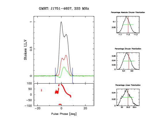
Figure 1: The left plot shows the time-averaged polarisation properties of PSR J1751-4657 at 333 MHz. The three panels in the right shows the distribution of the variation of $\%L$, $\%V$ and $\mid V\mid$ (from bottom to top) that arise due to the noise in the baseline. The red line shows the median of the distribution and the green line shows the rms. See section 4.1.2 for details. The figures for all pulsars is available for download (see appendix).

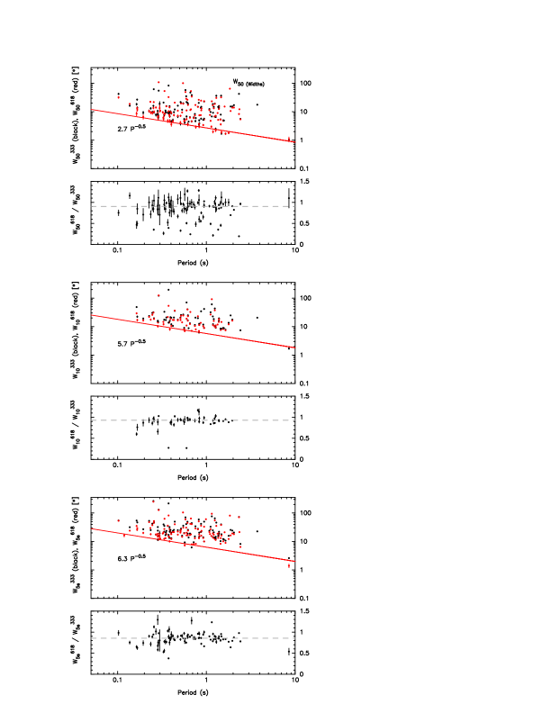
Figure 2: The three panels shows W₅₀, W₁₀ and $W_{5\sigma}$ width in our sample as given in table 3 as a function of pulsar period. The black and red points correspond to 333 MHz and 618 MHz respectively. The red lines in the figures correspond to 2.7${}^{\circ}P^{-0.5}$, 5.7${}^{\circ}P^{-0.5}$ and 6.3${}^{\circ}P^{-0.5}$ respectively. The bottom panel shows the ratio of the widths at the two frequencies as a function of pulsar period. The grey dashed lines are at 0.90, 0.92 and 0.84 respectively and shows the median values of the ratio. See section 4.1.2 for details.

Table 1: MSPES Observational Summary:

Freq	Total BW	Channel BW	tres	NTAP	NSP	Npol	NDrift
(MHz)	(MHz)	(MHz)	(msec)
333	16.66	0.065	0.245	105	83	59	39
618	16.66	0.065	0.245	118	93	49	44
Common	$-$	$-$	$-$	100	72	40	26

The first four columns of the table specifies the observing frequency, bandwidth, channel and time resolutions. Column 5 gives the number of pulsars N_TAP with good time-averaged polarization profiles, column 6 gives the number of pulsars N_SP for which the S/N ratio of the single pulse exceeds 5$\sigma$ limit and column 7 gives the number of pulsars where PPA’s can be measured for more than 5% of the single pulses. Column 8 specifies the number of pulsars N_Drift that showed drifting properties (see text for details).

4 RESULTS & DISCUSSION

We have recorded a total of 223 good average polarization profiles from 123 pulsars at two frequencies. In table 1 we present a short summary of the observations and in table 2 we summarize the observational results. Our sample has 77 pulsars common with GL98, and 30 pulsars common with JKMG08, which are the notable polarization surveys of pulsars at similar wavelengths, though our study had a significantly improved S/N. Additionally 79 pulsars in our sample were found to be common with the single pulse study of subpulse drifting by Weltevrede et al. (2007) and Weltevrede et al. (2006) using the Westerbork Synthesis Radio Telescope (WSRT) at 90 cm and 21 cm. There are 47 pulsars in our sample that were also in the list of the pulsars used for single pulse study by Burke-Spolaor et al. (2012) at 1350 MHz.

Most of the pulsars were observed for about 2100 pulses, however, in some cases we had fewer periods due to a variety of reasons like presence of RFI, setting of sources during the observing run, time on calibrator source, etc. The single pulse polarization study at 618 MHz, to the best of our knowledge, is the first such survey carried out at this frequency band. For each observed pulsar we determined the number of usable pulses (N_p), unaffected by RFI, along with the average S/N (S/N_avg) of the peak intensity for the entire observing run. We further estimated the percentage of single pulses for which the peak S/N $>$ 5 (see table 2). We found around 77% of the data, corresponding to 104 pulsars, useful for single pulse analysis (see table 1 for full summary). To give an assessment of the single pulse polarization quality we quote the percentage of single pulses in which polarization position angle (PPA) values for linear polarization S/N $>$ 3 could be measured. This gave around $\sim$50% of the pulsars which had more than 5% of the single pulses with measured PPA values (see table 1, 2). In the remainder of this section we discuss the preliminary outcomes of our survey.

4.1 Time Averaged properties

The time-averaged profiles, with periods of each pulsar determined using the $TEMPO2$ software, were obtained by averaging the single pulses, after rejecting the ones affected by RFI (an example of average polarization for the pulsar J1751–4657 is shown in Fig. 1). We estimated pulse widths at each frequency ($\nu$) using three different schemes namely the $W_{5\sigma}^{\nu}$ corresponding to the pulse width measured at five times the baseline noise rms and $W_{10}^{\nu}$ and $W_{50}^{\nu}$ corresponding to widths at 10% and 50% level of the peak intensity, respectively. All the measured widths at each frequency are shown in table 3 along with the error in pulse widths, computed using the prescription of Kijak & Gil 1997 (equation 4 therein). The average linear polarization $L(\phi_{i})$ across the profile phase, $\phi_{i}$, was obtained by summing up the stokes $U(\phi_{i})$ and $Q(\phi_{i})$ along each $\phi_{i}$, and using the relation $L(\phi_{i})=\sqrt{\left(\sum_{j=1}^{n}U_{j}(\phi_{i})\right)^{2}+\left(\sum_{j=1}^{n}Q_{j}(\phi_{i})\right)^{2}}/n$, here $n$ is the total number of pulses. The $L(\phi_{i})$ estimated above has a positive bias, and a mean value of the linear polarization obtained from the off pulse region is subtracted to obtain the final $L(\phi_{i})$. The average circular polarization was obtained using the relation $V(\phi_{i})=\sum_{j=1}^{n}V_{j}(\phi_{i})/n$. The average polarization position angle was obtained as $\Psi(\phi_{i})=$ 0.5 tan${}^{-1}\left(\sum_{j=1}^{n}U_{j}(\phi_{i})/\sum_{j=1}^{n}Q_{j}(\phi_{i})\right)$, with only points greater than three times the rms of the linear polarization baseline level being used.

4.1.1 Pulse widths

Pulse width serves as a useful tool for investigating the geometry and location of pulsar radio emission within the magnetosphere. In figure 2 we show the dependence of the different widths, W${}_{50}^{\nu}$, W${}_{10}^{\nu}$ and W${}_{5\sigma}^{\nu}$, on pulsar period $P$. In table 3 we have indicated 12 pulsars at 333 MHz and the pulsar J1848$-$0123 at 618 MHz which were highly scattered and not used in our plots and statistical analysis. The bottom panel in Fig. 2 shows the ratio of the widths at the two frequencies and the dashed grey line is the median value of the ratio. The average ratio of the three profile measure is $\sim$0.89, and agrees with the putative phenomenon of radius to frequency mapping (e.g. Mitra & Rankin 2002). Assuming a power law dependence of the frequency on widths, $W^{\nu}\propto\nu^{a}$, we find, $a\sim$-$0.19\pm 0.1$, which agrees with previous results (Mitra & Deshpande, 1999; Mitra & Rankin, 2002; Chen & Wang, 2014). There was one notable exception to the above results, PSR J1034–3224, where the ratio of widths was significantly larger than unity. On closer inspection it was revealed that an additional emission component appeared at 618 MHz which was absent at 333 MHz.

The pulse width decreasing with increasing $P$, seen in Fig. 2, is a well established phenomenon with a lower bound to the distribution of widths noted by several authors (e.g. Lyne & Manchester 1988; Rankin 1990, 1993, GL98, Maciesiak & Gil 2011; Maciesiak et al. 2012; Pilia et al. 2015). In particular Rankin (1990) found that $W_{50}$ for the core components followed a lower boundary line (LBL) corresponding to $2.45^{\circ}P^{-0.5}$ where the $P^{-0.5}$ dependence is the scaling of the opening angle of the open dipolar field lines (e.g. Biggs 1990,Kramer et al. 1998). Recently Maciesiak et al. (2012) emphasized the existence of the same LBL, $2.45^{\circ}P^{-0.5}$, for $W_{50}$ at 1 GHz frequency in a wider population of 1450 pulsars, which included both core and conal components. They argued that the LBL corresponds to the smallest angular structures that can be observed either as core or conal component widths. In Fig. 2 the width distribution also appears to have a lower bound. Since the pulse widths at 618 MHz are smaller, the lower bound is dominated by the 618 MHz measurements. We modeled the lower bound for $W_{50}$ by scaling the 1 GHz value of 2.45^∘ to 618 MHz using $\alpha\sim$-$0.19$ and find the LBL to be $2.7^{\circ}P^{-0.5}$ which appears to be consistent with our result. In the case of widths $W_{10}$ and $W_{5\sigma}$ we observed LBLs but there are no previous estimates to compare our results. The lower bounds, which are dominated by measurements at 618 MHz for $W_{10}$ and $W_{5\sigma}$, could be represented by a LBL of the form $5.7^{\circ}P^{-0.5}$ and $6.3^{\circ}P^{-0.5}$ respectively, and were derived by visual examination. Since the $W_{10}$ and $W_{5\sigma}$ are measured at comparatively lower intensity levels that $W_{50}$, these measurements includes both the width of the component as well as the separation of the components. Thus the fact that in these measurements the period scaling of $P^{-0.5}$ still seem to hold implies that the spacing between the components has a similar period scaling as the component ($W_{50}$) widths. The presence of a LBL in the width distribution is a curious phenomenon and a more detailed study to understand the LBL as a function of pulsar frequency and other profile measures is currently underway.

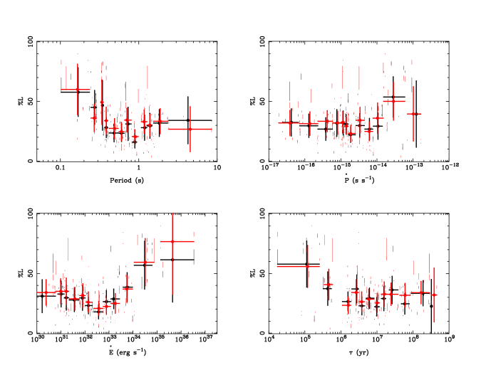
Figure 3: The percentage of linear polarization for all the observed pulsars (table 2) is plotted as a function of different pulsar parameters. The black and red short lines correspond to 333 MHz and 618 MHz respectively. The black and red points with error bars correspond to median values of the sample. See section 4.1.2 for details.

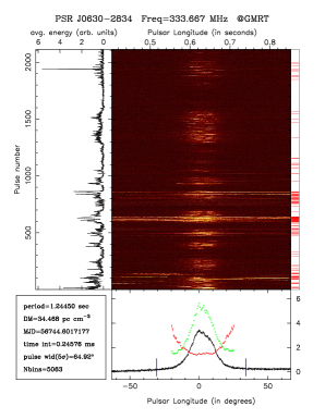
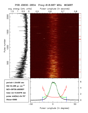
Figure 4: The central panel on the left and right plots show single pulse stacks of PSR J0630-2834 at 333 and 618 MHz respectively. The red horizontal lines on the rightmost strip correspond to pulses affected by RFI. The blue vertical bars in the bottom plot correspond to the leading and trailing edge of the pulse estimated at 5$\sigma$ level, the black curve corresponds to the average total intensity, the green points in the bottom panel are the rms of the intensity fluctuation along each longitude and the red points show the modulation index. The black curve in the left panel shows the variation of the average single pulse intensity as a function of pulse number. See section 4.2.1 for detail. The figures for all pulsars are available for download (see appendix).

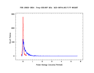
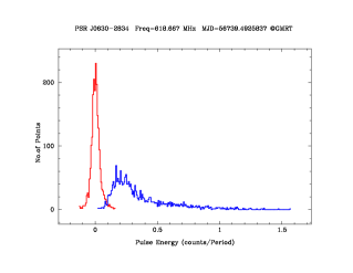
Figure 5: The left and right plots show the off-pulse (red curves) and on-pulse (blue curves) energy histograms for PSR J0630-2834 based on the data in figure 4 for 333 and 618 MHz respectively. See section 4.2.1 for detail. The figures for all pulsars are available for download (see appendix).

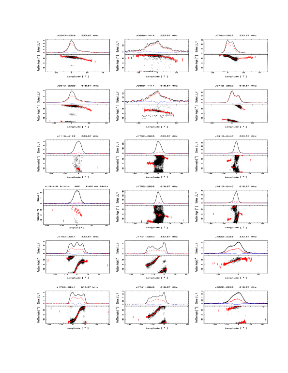
Figure 6: Example of single pulse polarization position angle (PPA) histograms for three different ranges of $\dot{E}$, with three pulsars shown for each range at both 333 and 618 MHz. The top two panels correspond to $\dot{E}>10^{34}$ erg s^-1, middle two panels correspond to $\dot{E}\sim 10^{32}-10^{34}$ erg s^-1 and bottom two panels corresponds to $\dot{E}<10^{31}$ erg s^-1. A running mean of 3 bins has been applied to the data before plotting to increase the S/N of the PPA points. The figures for all pulsars are available for download (see appendix).

4.1.2 Average polarization properties

In table. 3 we list the average degree of linear $\%L=\sum_{i}L(\phi_{i})/I(\phi_{i})$, circular $\%V=\sum_{i}V(\phi_{i})/I(\phi_{i})$ and absolute circular $\%\mid V\mid=\sum_{i}\mid V(\phi_{i})\mid/I(\phi_{i})$ polarization where the summation is across pulse phase $\phi_{i}$ and is performed for only statistically significant values, i.e. with S/N $>$ 3, for the respective quantities, and the noise were estimated from the off-pulse region. It is to be noted that while Stokes $I,Q,U$ and $V$ have errors with gaussian distribution, the quantities $\%L$, $\%V$ and $\%\mid V\mid$ have non-gaussian error distributions and hence error estimates for these quantities cannot be computed using standard error propagation (Mitra et al., 2015). Instead we took the following approach to estimate the errors. Using the noise rms obtained from the off pulse region, we constructed a large number of profiles by varying each of the four stoke parameters randomly within the rms value. For each of these profiles we estimated the average $\%L,\%V$ and $\%\mid V\mid$ as described above. The median and the rms values of this distribution were used as estimates and errors respectively. Figure 1 shows the details of these measurements for one pulsar. In a number of cases, PSR J1648–3256, J1848–1414, J1849–0636 and J1921+1948 at 333 MHz and PSR J1739–2903 (main pulse), J1757–2421, J1835–1020, J1848–1414 and J1921+1948 at 618 MHz, there were insufficient polarization measurements above the rms cutoff to yield any average polarization values despite the total intensity profile having sufficient signal to noise. These are examples of extreme depolarization in the pulsar population.

The degree of polarization has been shown to be correlated with pulsar period $P$, period derivative $\dot{P}$ and their derived parameters particularly the spindown energy loss $\dot{E}=4\pi^{2}I\dot{P}P^{-3}$ erg s^-1 where $I$ is the moment of inertia having a typical value of 10⁴⁵ g cm², and characteristic age $\tau=0.5P\dot{P}^{-1}$ yr (Von Hoensbroech 1998; von Hoensbroech et al. 1998, GL98, Crawford et al. 2001; Han et al. 2009; Weltevrede & Johnston 2008, hereafter WJ08). The strongest correlation is observed between $\%L$ and $\dot{E}$, with high $\dot{E}$ pulsars showing higher degree of linear polarization. The correlation was a highlight of the study conducted by WJ08 at 1.4 GHz using 350 pulsars in the $\dot{E}$ range $\sim 10^{30}-10^{37.5}$ erg s^-1, where a distinct but gradual transition is seen around $\dot{E}\sim 10^{34}-10^{35}$ erg s^-1, above which the degree of polarization is very high with a mean value of 60% and below this level it decreases to 20%. A similar correlation in the meterwavelengths has also been reported by GL98. We have observed similar correlations in our data where the dependence of $\%L$ with $P$, $\dot{P}$, $\dot{E}$ and $\tau$ is shown in figure 3. It is to be noted that there exists a spread in the measured values of the degree of polarization along all $\dot{E}$, however the mean values obtained by dividing the data along multiple bins in $\dot{E}$ reveal clear trends in agreement with WJ08. The minimum of the mean linear polarization is about 20% at $\dot{E}\sim 10^{32.3}$ erg s^-1, which rises marginally to 30% below this level but increases significantly to 70% in the higher $\dot{E}$ range. Another interesting dependence of $\%L$ on $\tau$ is observed where younger pulsars ($\tau<10^{6}$ yr) show very high polarizations upto 70% compared to older ones ($\tau\gg 10^{6}$ yr) with $\%L\sim 30\%$. Our data shows no evidence for any correlation for $\%V$ and $\%\mid V\mid$ to any of these pulsar parameters.

4.2 Single Pulse Properties

The observed pulsed emission can be analysed in a number of ways as illustrated in figures 4 and 5 for the pulsar J0630$-$2834 and figure 6 at the two observing frequencies. The data can be used to study pulsar phenomenon involving both single pulse total intensity and single pulse polarization.

4.2.1 Single pulse total intensity

A useful way of plotting single pulse data are single pulse stacks where the intensity corresponding to consecutive pulsar period is plotted on top of each other as shown in figure 4. The main panel in the plot represents colour coded contour of single pulse stack of total intensity $I(j,\phi_{i})$ , which corresponds to the $j^{\rm{th}}$ pulse along the y-axis and the pulse phase $\phi_{i}$ along the x-axis. The baseline levels for each of the single pulses were estimated from a region of minimum rms in the off-pulse window which was subtracted from each pulse to create the stack. In addition the pulses affected by RFI were identified using a statistical approach, determining the mean and rms in a off-pulse window for each pulse where the pulses exceeding five times the median noise identified as outliers, and shown on the rightmost strip of the figure (horizontal red lines). The outlier pulses were not included in subsequent analysis. The on-pulse window bounded by the longitude range $n_{1}$ and $n_{2}$ was determined as the region above 5 times the rms of the off-pulse window and marked with blue bordering lines. The average energy corresponding to each single pulse was determined as $\sum_{i=n_{1}}^{n_{2}}I(j,\phi_{i})/N_{{\rm bins}}$ within the on-pulse window having $N_{{\rm bins}}$ number of bins, and is shown as the black curve on the left panel. The average profile after rejecting the RFI affected pulses is shown as the black curve in the lowermost panel. In addition we have also estimated the fluctuation of the pulse to pulse intensity along every longitude $\phi_{i}$ by measuring the rms of $I(j,\phi_{i})$ which is shown as the green points in the lowermost panel. The longitude resolved modulation index $m(\phi_{i})$ is shown as the red points with errorbars in the lowermost panel, and is defined as $m(\phi_{i})=\left(\sqrt{<I(j,\phi_{i})^{2}>-<I(j,\phi_{i})>^{2}}\right)/<I(j,\phi_{i})>$ where the angle brackets indicate mean values, and the errors were estimated using Monte Carlo simulations (see Weltevrede et al. 2012). The MSPES data set showed a rich variety in the distribution of on-pulse energy of single pulse intensity which are related to phenomenon like pulsar nulling, moding (e.g. Wang et al. 2007) and interstellar scintillation (e.g. Rickett 1977). This variation can be effectively represented by plotting on-pulse and off-pulse energy histogram of single pulses (see Ritchings 1976), an example of which is shown for PSR J0630-2834 in figure 5. The red histogram corresponds to the off-pulse energy histogram which was computed by first finding a off-pulse window in the average profile which corresponds to a minimum rms regions, and then using the same window to find the mean energies of the single pulses. For purely white noise the off-pulse histogram should have a normal distribution. However, as seen in figure 5 the distribution, particularly at 333 MHz is asymetric, and arises due to a presence of gain variations leading to systematics in the baseline level, and low level RFI which could not be detected through our RFI excision algorithm. The on-pulse histogram is the blue histogram in figure 5, and was computed by finding the single pulse energy in the on-pulse window corresponding to 5$\sigma$ pulse width. The on-pulse energy distribution has contribution from the low level RFI and baseline variations as well as from pulsar single pulse phenomenon associated with nulling, moding and scintillation. A proper investigation of these phenomenon will need to address the issue of mitigating the low level RFI and baseline systematics (one method to eliminate baseline systematics have been devised in MSPESII, appendix A). Currently more detailed study of these phenomenon are underway and will be reported elsewhere.

The next important single pulse phenomenon is subpulse drifting. The pulsed emission is composed of one or more components called subpulses which in certain pulsars is seen to exhibit periodic variation. This phenomenon is known as subpulse drifting and has been a subject of considerable interest for understanding the radio emission mechanism. The largest study of subpulse drifting has been conducted by Weltevrede et al. (2006, 2007) where 187 pulsars were studied and drifting features reported in 68 pulsars with 42 new detections. A comprehensive study of the phenomenon of drifting subpulses using the present dataset has been carried out by Basu et al. (2016, hereafter MSPESII) which is being presented as an accompanying paper. The principal outcomes of the studies are as follows: we detected drifting features in 39 pulsars at 333 MHz, and 44 pulsars at 618 MHz with a total of 57 pulsars showing some features of drifting. The drifting phenomenon was detected for the first time in 22 pulsars which increased the sample of drifting pulsars by around 20% and is one of the largest such studies conducted. In table 2 pulsars showing drifting are indicated as “D” and the new detections are indicated as “D^⋆”. As demonstrated in MSPESII, the superior quality of single-pulses in the current study enabled us to estimate the drifting properties with much higher significance.

4.2.2 Single Pulse Polarization

Several examples of single pulse polarisation are shown in figure 6. The plot represents the distribution of the single pulse phased-resolved PPA (grayscale), with only statistically significant points exceeding three times the off-pulse noise levels shown in the plot. The average PPA is overlaid as a red curve. We found around 60% of the pulsars in our sample to exhibit PPA histograms with some discernible points within the pulse window (see table 2). The circular polarization of the single pulses were weak for most pulsars barring a few bright cases, which will be studied in a future paper.

The PPA histograms exhibit a variety of shapes ranging from simple S-shaped curves (RVM) to extremely complex structures. In some cases the two orthogonal polarization tracks are clearly visible. The PPA values are determined within (-90,+90) degrees and at any given longitude there are two distinct distributions. A tightly bunched distribution confined to around 10-20 degrees, mostly seen in pulsars with S-shaped PPA tracks, and a wide spread which sometimes cover the entire window. Despite a large variation in shape, a pattern connecting the PPA histogram and the average degree of linear polarization emerges in our sample. In figure 6 we show examples of pulsars with three distinct PPA behaviour at 333 MHz and 610 MHz: (1) the top two panels show pulsars with high linear polarization, $\%L\sim 60-70\%$, which are typically associated with $\dot{E}\geq 10^{34}$ erg s^-1. The single pulse polarization in these cases are close to the average value and the PPA histograms show tight bunching, sometimes with a hint of weak orthogonal polarization modes. (2) The middle two panels are examples of pulsars with extremely low linear polarization, $\%L<10\%$, associated with $\dot{E}$ between 10³² and 10³⁴ erg s^-1. The PPA histograms show chaotic shapes with random spread within the window. (3) The bottom two panels are examples of pulsars with intermediate polarizations, $\%L\sim 30\%$ and $\dot{E}<10^{32}$ erg s^-1 cases. These typify PPA with low spread, resembling the RVM, and exhibit clear orthogonal polarization modes. A detailed study of single pulse polarization and how it leads to depolarization in average profiles will be presented elsewhere.

5 Summary

In this paper we have described the time-averaged and single pulse emission properties of the pulsars in MSPES conducted using the GMRT at 333 MHz and 618 MHz. These observations were aimed at a systematic and detailed study of the pulsar radio emission properties. The calibrated data sets (section 3) have been used to estimate the pulse widths and average linear and circular polarizations in the pulsar sample (table 3 and discussion in section 4). The effect of RFM is clearly demonstrated in the pulse widths with an estimated power law index of $a\sim$-$0.19$ for the evolution of widths between 333 MHz and 618 MHz. The pulse width distribution with period had a lower bound, with the LBL corresponding to 2.7${}^{\circ}P^{-0.5}$, 5.7$P^{-0.5}$ and 6.3$P^{-0.5}$ for $W_{50}$, $W_{10}$ and $W_{5\sigma}$ respectively at 618 MHz. The LBL for $W_{50}$ at 1.4 GHz was found to be 2.45${}^{\circ}P^{-0.5}$ by Maciesiak et al. (2012) and interpreted as emission from the narrowest angular structure, mainly the core/conal component, in a pulse profile. They invoke the partially screened vacuum gap (PSG) model (Gil et al., 2003) of the inner accelerating region which was initially suggested by Ruderman & Sutherland (1975), and argue that the components in a pulse profile are related to the sparking discharge in the PSG. They further demonstrate that the numerical factor $\sim$2.45^∘ in the $W_{50}$ widths can be related to the radius of curvature of non-dipolar magnetic field in the PSG where dense electron-positron plasma is created due to the sparking process and finally the pulsar radio emission arises at altitudes of about 50 stellar radii above the neutron star surface. Our result for $W_{50}$ LBL support the findings of Maciesiak et al. (2012), where the slightly higher numerical factor 2.7^∘ at 618 MHz can be attributed to RFM. The $W_{10}$ and $W_{5\sigma}$ LBL however is not connected to the component widths, instead they measure widths for both the components and the separation of the components and the LBL suggests the non existence of pulsed radio emission structures below this level in the pulsar population. The $P^{-0.5}$ dependence of the widths follows from the nature of the dipolar open magnetic field lines in the radio emission region. The physical origin of this bound is currently unclear.

We found $\%L$ to be correlated with various pulsar parameters confirming previous studies. The degree of correlation varies with various parameters, e.g. it is much stronger with $P$ than $\dot{P}$. $\%L$ is seen to be as high as 70% for pulsars rotating faster than $\sim$300 milliseconds and about 30% for periods slower than 400 milliseconds. The correlation of $\%L$ is also present with both $\dot{E}$ and $\tau$, where $\%L$ is 70% for $\dot{E}>10^{35}$ erg s^-1 and $\tau<10^{5.5}$ yr and $\%L$ is 30% for $\dot{E}<10^{34}$ erg s^-1 and $\tau>10^{6}$ yr. The physics of depolarization in pulsars is still poorly understood, which makes these results, particularly the transitions between high and low $\%L$, as important inputs into the various models. One likely source of depolarization is the presence of orthogonal and non-orthogonal polarization modes (e.g. Rankin & Ramachandran, 2003). Our single pulse polarization data showed that several pulsars with low $\%L$ exhibit a variety of OPM and non-OPM distributions compared to high $\%L$ pulsars. A detailed single pulse study revealing the relation between polarization properties of individual pulses and average pulses is essential to understand the depolarization process. Additionally, the high quality single pulse data obtained in our survey showed clear presence of nulling and subpulse drifting. In an accompanying paper, MSPESII, a detailed study of drifting subpulses revealed that around 45% of the pulsars in our sample exhibit drifting features with 22 pulsars in which this phenomenon was detected for the first time as indicated in table 2.

Our data is consistent with the observational evidence that the coherent radio emission in pulsars originating at heights of 50 stellar radii or below 10% of the light cylinder (Blaskiewicz et al., 1991; Rankin, 1993; Kijak & Gil, 1997) which suggests the presence of strong magnetic fields ($\sim 10^{8}$ G) in the emission region. In such strong magnetic fields the radio emitting plasma is constrained to move only along the field lines with all transverse motions suspended. In this specialized condition only the two-stream instability can develop within the plasma and our current understanding is that the non-linear growth of the two stream instability can lead to formation of charged relativistic solitons emitting coherent curvature radiation in plasma (Melikidze et al., 2000; Gil et al., 2004; Mitra et al., 2009; Melikidze et al., 2014). The supply of the radio emitting plasma from the inner accelerating region is initiated by a sparking process (e.g Ruderman & Sutherland, 1975) and the drifting subpulse phenomenon is thought to be associated with the $\vec{E}\times\vec{B}$ drift, where $\vec{E}$ and $\vec{B}$ are the electric and magnetic fields in the inner accelerating region. The detailed study of the drifting subpulse phenomenon of our data in MSPESII confirms the presence of the inner accelerating region and favours the PSG model. However major challenges are faced when the coherent curvature radiation theory is used to explain the polarization properties. The curvature radiation can excite the ordinary ordinary (O-mode) and extraordinary (X-mode) modes within the plasma (Melikidze et al., 2000; Gil et al., 2004; Mitra et al., 2009; Melikidze et al., 2014). The X-mode, with the waves polarized perpendicular to the magnetic field planes, can emerge from the plasma without suffering any propagation effect. This is supported by good observational evidence where the linear polarization vector emerges from the pulsar as X-mode (Lai et al., 2001; Johnston et al., 2005; Rankin, 2015). The presence of OPMs on the other hand also suggests the emergence of the O-modes where the polarization is in the plane of the magnetic field line. However, theoretically considerations expect the O-modes to be heavily damped within the plasma and unable to emerge (Arons & Barnard 1986,Melikidze et al. 2014). Also there is no theoretical basis to understand the presence of circular polarization observed in pulsars. We aim to carry out a systematic study of identifying the OPM in our large sample to better understand the polarization properties in pulsars.

The data presented in this paper as well as other studies strongly suggest that the emission properties depend on pulsar parameters, particularly $\dot{E}$. It appears that $\dot{E}$ change leads to a systematic change in the radio emitting plasma, thereby affecting the pulsar emission properties. Our future aim is to use these observational results and perform further detailed analysis of emission properties to enhance our understanding of the physics of pulsar radio emission under the framework of the coherent curvature radio emission model, with our present work being a significant attempt towards these goals.

Appendix

We have made the plots and data products from our survey freely available to the user.

Several of the data products for each pulsar have been archived in the website:
http://mspes.ia.uz.zgora.pl/

The bulk download of files is also available from:
ftp://ftpnkn.ncra.tifr.res.in/dmitra/MSPES/

Table 2: The table gives the sample of pulsars observed. The first 8 columns gives various pulsar parameter obtained from the ATNF pulsar catalog. In the rotation measure (RM) column the quantities with (NA) are pulsars for which RM was not available in the ATNF catalog. Columns 9$-$13 gives single pulse properties for 333 MHz data where we give the number of single pulses N_p which are not affected due to RFI, the average peak signal to noise ratio S/N_avg, the percentage of pulses f_5σ for which the peak signal to noise ratio exceeds the 5 times the off-pulse rms and the percentage of single pulses f_pol for which single pulse polarization is detected. f_pol is only quoted when the number of pulses exceeds 100. Columns 14$-$18 corresponds to 618 MHz data. The letters D in column 13 and 18 stands for pulsars showing drifting features, while D^∗ represents drifting reported for the first time (see MSPESII).

								333 MHz					618 MHz
	Jname	Period	$\dot{P}_{-15}$	DM	RM	$\tau_{6}$	$\dot{E}_{31}$	Np	S/Navg	f5σ	fpol		Np	S/Navg	f5σ	fpol
		(s)	(s s-1)	($\frac{\rm{pc}}{\rm{cc}}$)	($\frac{\rm{rad}}{\rm{m}^{2}}$)	(yr)	(erg s-1)			(%)	(%)				(%)	(%)
1	J0034-0721	0.942	0.4080	10.92	9.89	36.6	1.92	2042	13.3	62	54	D	1124	5.7	40	19	D
2	J0134-2937	0.136	0.0784	21.81	13.00	27.7	120	2180	3.7	$<$5	$<$5		2144	3.1	$<$5	$<$5
3	J0151-0635	1.464	0.4436	25.66	2.00	52.4	0.556	615	5.6	44	11	D	519	5.5	40	25	D
4	J0152-1637	0.832	1.30	11.93	2.00	10.2	8.88	2054	10.8	93	39	D	2079	8.7	88	24	D
5	J0206-4028	0.630	1.20	12.90	-4.00	8.33	18.9	1993	6.3	71	7		2080	3.1	$<$5	$<$5
6	J0304+1932	1.387	1.30	15.74	-8.30	17.0	1.91	2058	13.1	81	68	D	2026	8.5	72	56	D
7	J0452-1759	0.548	5.75	39.90	13.80	1.51	137	1868	20.9	99	86		2158	8.0	85	33
8	J0525+1115	0.354	0.0736	79.34	37.00	76.3	6.53	1872	4.5	26	$<$5	D	2169	3.4	$<$5	$<$5
9	J0528+2200	3.745	40.1	50.94	-39.60	1.48	3.01	444	18.4	74	74		—	—	—	—
10	J0543+2329	0.245	15.4	77.71	8.70	0.253	4090	2118	7.7	49	37		2188	9.3	57	42
11	J0614+2229	0.334	59.4	96.91	69.00	0.089	6240	2029	4.1	17	7		1989	3.0	$<$5	$<$5
12	J0629+2415	0.476	2.00	84.19	69.50	3.78	72.8	1993	11.2	98	71		2079	5.8	67	11
13	J0630-2834	1.244	7.12	34.42	46.53	2.77	14.6	1934	6.8	46	35		2079	9.9	86	70	D
14	J0659+1414	0.384	55.0	13.98	23.50	0.111	3810	2128	5.7	27	14		2152	4.3	19	8
15	J0729-1836	0.510	19.0	61.29	51.00	0.426	564	2061	7.0	54	21		2099	4.6	24	5
16	J0738-4042	0.374	1.62	160.80	12.10	3.68	121	2194	4.9	41	4		2188	8.9	93	47
17	J0742-2822	0.166	16.8	73.78	149.95	0.157	14300	1741	24.2	100	99		1767	21.6	100	99
18	J0758-1528	0.682	1.62	63.33	55.00	6.68	20.1	2079	3.2	6	$<$5		2067	5.0	38	$<$5	D
19	J0820-1350	1.238	2.11	40.94	-1.20	9.32	4.38	327	36.0	98	—	D	2063	8.4	97	35	D
20	J0820-4114	0.545	0.0189	113.40	57.70	4578	0.460	—	—	—	—		2161	3.9	6	$<$5
21	J0837+0610	1.273	6.80	12.86	25.32	2.97	13.0	1036	50.6	94	93	D	2026	11.9	92	64	D
22	J0846-3533	1.116	1.60	94.16	144.00	0.110	4.55	1964	3.9	7	$<$5	D∗	2090	3.8	$<$5	$<$5	D∗
23	J0905-4536	0.988	0.149	179.70	153.00	105	0.609	—	—	—	—		2057	3.1	$<$5	$<$5
24	J0905-5127	0.346	24.9	196.43	291.00	0.22	2370	2247	3.1	$<$5	$<$5		3454	3.1	$<$5	$<$5
25	J0908-1739	0.401	0.669	15.88	-31.00	9.50	40.8	2050	3.8	15	$<$5		2229	3.4	6	$<$5
26	J0922+0638	0.430	13.7	27.30	29.20	0.497	679	2202	8.5	93	50		2222	7.7	83	44
27	J0944-1354	0.570	0.0453	12.50	-7.00	200	0.963	1961	9.8	88	67	D	2191	3.7	6	$<$5
28	J0953+0755	0.253	0.230	2.97	-0.66	17.5	56.0	1063	177.2	97	96		2215	137.3	99	98
29	J0959-4809	0.670	0.0820	92.70	50.00	129	1.08	—	—	—	—		1973	4.0	11	$<$5	D∗
30	J1034-3224	1.150	0.230	50.75	-8.00	79.1	0.597	1528	6.5	53	11	D∗	2125	4.7	23	9	D∗
31	J1041-1942	1.386	0.945	33.78	-16.00	23.2	1.40	—	—	—	—		2040	4.8	31	13	D
32	J1116-4122	0.943	7.95	40.53	-37.00	1.88	37.4	2090	5.0	34	5	D∗	1905	4.6	30	$<$5
33	J1136+1551	1.187	3.73	4.85	3.97	5.04	8.79	725	16.4	61	48		401	21.2	80	70
34	J1239+2453	1.382	0.960	9.26	-0.12	22.8	1.43	1033	33.2	94	90	D	860	12.4	85	69	D
35	J1257-1027	0.617	0.363	29.63	8.00	27.0	6.09	2022	5.0	37	$<$5		2101	3.7	11	$<$5
36	J1321+8323	0.670	0.566	13.31	-20 (NA)	18.7	7.43	—	—	—	—		1963	3.5	6	$<$5
37	J1328-4357	0.532	3.01	42.00	-41.00	2.80	78.7	2004	3.5	5	$<$5		2047	4.0	13	$<$5
38	J1328-4921	1.478	0.610	118.00	170.00	38.4	0.745	2019	6.6	44	15	D∗	2000	4.6	28	$<$5	D∗
39	J1418-3921	1.096	0.889	60.49	-15.00	19.5	2.66	—	—	—	—		866	3.6	$<$5	$<$5	D∗
40	J1507-4352	0.286	1.60	48.70	-34.00	2.83	269	2124	3.5	$<$5	$<$5		2266	3.1	$<$5	$<$5
41	J1527-3931	2.417	19.1	49.00	4.00	2.01	5.33	858	6.3	70	55	D∗	1193	3.6	$<$5	$<$5
42	J1549-4848	0.288	14.1	55.98	-15.00	0.324	2320	2155	3.2	$<$5	$<$5		2289	2.7	$<$5	$<$5
43	J1555-3134	0.518	0.0622	73.05	-49.00	132	1.77	2036	4.7	34	$<$5	D∗	2181	4.7	34	$<$5	D∗
44	J1557-4258	0.329	0.330	144.50	-41.90	15.8	36.5	2155	3.4	$<$5	$<$5		2146	4.3	30	5
45	J1559-4438	0.257	1.02	56.10	-7.00	4.00	237	2235	7.1	84	35		2478	14.1	100	98
46	J1602-5100	0.864	69.6	170.93	71.50	0.197	426	2128	3.7	$<$5	$<$5		4208	6.2	60	4
47	J1603-2531	0.283	1.59	53.76	15.00	2.82	277	2046	2.8	$<$5	$<$5		2104	3.4	8	$<$5	D∗
48	J1604-4909	0.327	1.02	140.80	-16.00	5.09	115	—	—	—	—		2165	5.3	44	$<$5	D∗
49	J1625-4048	2.355	0.443	145.00	-7.00	84.2	0.134	—	—	—	—		1520	3.2	5	$<$5	D∗
50	J1637-4553	0.118	3.19	193.23	10.00	0.59	7510	2482	—	$<$5	$<$5		2482	2.6	$<$5	$<$5
51	J1645-0317	0.387	1.78	35.76	15.80	3.45	121	—	—	—	—		2154	90.5	100	99	D
52	J1648-3256	0.719	3.53	128.28	-60.00	3.23	37.4	1638	3.4	$<$5	$<$5		2054	3.0	$<$5	$<$5
53	J1700-3312	1.358	4.71	166.97	-15.00	4.57	7.42	2076	3.2	$<$5	$<$5		2101	3.7	7	$<$5	D∗
54	J1703-3241	1.211	0.660	110.31	-21.70	29.1	1.46	1646	7.5	82	52	D∗	2039	7.6	89	61	D∗
55	J1705-3423	0.255	1.08	146.36	-44.00	3.7	255	2182	3.4	$<$5	$<$5		2088	3.6	$<$5	$<$5
56	J1709-1640	0.653	6.31	24.89	-1.30	1.64	89.4	1909	15.5	88	73		2059	8.2	76	35
57	J1709-4429	0.102	93.0	75.69	0.70	0.017	341000	2876	3.3	$<$5	$<$5		2876	3.5	$<$5	$<$5
58	J1720-2933	0.620	0.746	42.64	21.00	13.2	12.3	2039	5.3	54	5	D	2125	5.7	56	7	D
59	J1722-3207	0.477	0.646	126.06	90.00	11.7	23.5	2107	4.2	8	$<$5		2108	4.1	11	$<$5	D∗
60	J1722-3712	0.236	10.9	99.50	104.00	0.345	3250	2286	3.2	$<$5	$<$5		2286	3.2	$<$5	$<$5
61	J1727-2739	1.293	1.10	147.00	0.0(NA)	18.6	2.01	2030	3.0	$<$5	$<$5		2094	2.8	$<$5	$<$5
62	J1731-4744	0.829	164	123.33	-429.10	0.080	1130	2135	17.8	98	80		2157	29.0	100	95
63	J1733-2228	0.871	0.0427	41.14	-12.00	323	0.255	2009	5.2	45	7	D	2099	3.8	$<$5	$<$5	D
64	J1733-3716	0.337	15.0	153.50	-335.00	0.355	1540	—	—	—	—		1959	2.9	$<$5	$<$5	D∗
65	J1735-0724	0.419	1.21	73.51	38.00	5.47	65.0	2105	11.6	81	50	D	2146	5.1	44	$<$5	D
66	J1739-2903	0.322	7.88	138.56	-236.00	0.649	924	—	—	—	—		2145	3.1	$<$5	$<$5
67	J1740+1311	0.803	1.45	48.67	64.40	8.77	11.1	2090	7.3	81	24		2137	7.6	73	38	D
68	J1741-0840	2.043	2.27	74.90	124.00	14.2	1.05	1709	5.1	33	30	D	2035	4.4	22	20	D
69	J1741-3927	0.512	1.93	158.50	204.00	4.20	56.7	2088	4.0	10	$<$5	D∗	2108	5.4	40	9	D∗
70	J1745-3040	0.367	10.7	88.37	101.00	0.546	849	2122	3.8	11	$<$5		2121	9.3	41	25
71	J1748-1300	0.394	1.21	99.36	67.00	5.15	78.2	2074	4.2	16	$<$5	D∗	2113	3.8	7	$<$5
72	J1750-3503	0.684	0.0381	189.35	173.00	284	0.470	2100	3.4	$<$5	$<$5		2095	3.4	$<$5	$<$5
73	J1751-4657	0.742	1.29	20.40	19.00	9.11	12.5	1938	14.9	95	88		1975	10.9	90	58
74	J1752-2806	0.562	8.13	50.37	96.00	1.10	180	2130	48.4	100	96		2128	70.3	97	95
75	J1757-2421	0.234	12.9	179.45	16.00	0.287	3980	—	—	—	—		2303	3.1	$<$5	$<$5
76	J1801-0357	0.921	3.31	120.37	32.00	4.41	16.7	2116	4.0	18	$<$5	D∗	1606	3.8	17	$<$5	D∗
77	J1801-2920	1.081	3.29	125.61	-62.00	5.21	10.3	2081	4.2	18	5		2106	3.7	8	$<$5	D∗
78	J1807-0847	0.163	0.0288	112.38	166.00	90.1	25.9	2195	4.0	11	$<$5		2200	6.8	78	$<$5
79	J1808-0813	0.876	1.24	151.27	77.00	11.2	7.28	2112	3.3	$<$5	$<$5		1550	3.5	$<$5	$<$5
80	J1816-2650	0.592	0.0664	128.12	90.00	141	1.26	1999	3.6	$<$5	$<$5	D∗	2114	3.3	$<$5	$<$5
81	J1817-3618	0.387	2.05	94.30	66.00	3.00	139	2116	5.2	33	9		—	—	—	—
82	J1817-3837	0.384	0.580	102.85	102.90	10.5	40.3	2129	3.0	$<$5	$<$5		2173	3.0	$<$5	$<$5
83	J1820-0427	0.598	6.33	84.44	69.20	1.50	117	2091	18.2	100	60		2090	12.1	99	48
84	J1822-2256	1.874	1.35	121.20	124.00	21.9	0.812	2059	4.5	27	7	D	1262	4.7	36	15	D
85	J1823-0154	0.759	1.13	135.87	153.00	10.6	10.2	2128	3.1	$<$5	$<$5		2043	3.3	$<$5	$<$5
86	J1823-3106	0.284	2.93	50.24	95.00	1.54	504	2058	8.8	85	44		2057	4.2	22	$<$5
87	J1823+0550	0.752	0.227	66.78	145.00	52.6	2.10	2263	9.2	74	24		2144	3.6	$<$5	$<$5
88	J1834-0426	0.290	0.0719	79.31	100.00	63.9	11.6	2254	4.5	22	$<$5		2244	4.3	15	$<$5
89	J1835-1020	0.302	5.92	113.70	0.0(NA)	0.810	845	—	—	—	—		2167	2.9	$<$5	$<$5
90	J1835-1106	0.165	20.6	132.68	42.00	0.128	17800	3554	3.2	$<$5	$<$5		2171	3.1	$<$5	$<$5
91	J1841+0912	0.381	1.09	49.11	53.00	5.54	77.6	2134	3.2	$<$5	$<$5		2131	3.6	6	$<$5
92	J1842-0359	1.839	0.509	195.98	326.00	57.3	0.322	1871	3.8	$<$5	$<$5	D	1925	4.1	13	$<$5	D
93	J1843-0000	0.880	7.79	101.50	0.0(NA)	1.79	0.451	1962	3.5	$<$5	$<$5		2087	3.6	$<$5	$<$5
94	J1844+1454	0.375	1.87	41.50	109.00	3.18	140	2121	4.9	41	$<$5		2223	3.3	$<$5	$<$5
95	J1847-0402	0.597	50.17	141.98	117.00	0.183	956	2072	4.1	8	$<$5		2070	4.2	16	$<$5
96	J1848-0123	0.659	5.25	159.53	580.00	1.99	72.3	2180	3.7	$<$5	$<$5		2113	4.4	18	$<$5	D
97	J1848-1414	0.297	0.0141	134.47	0.0(NA)	335	2.11	2171	2.9	$<$5	$<$5		2192	2.8	$<$5	$<$5
98	J1849-0636	1.451	40.62	148.17	-35.00	0.497	59.7	2066	4.3	19	$<$5		2068	5.3	24	$<$5
99	J1852-2610	0.336	0.0877	56.81	-21.00	60.8	9.10	2062	4.0	12	$<$5		1900	3.3	$<$5	$<$5
100	J1900-2600	0.612	0.205	37.99	-2.30	47.4	3.52	1976	12.9	85	68	D	2095	6.4	70	34	D
101	J1901-0906	1.781	1.64	72.68	29.00	17.2	1.14	2012	5.7	42	29	D	1049	4.7	28	12	D
102	J1909+1102	0.283	2.64	149.98	540.00	1.70	457	2022	6.9	73	26	D	2061	5.7	60	8	D
103	J1910+0358	2.330	4.47	82.93	-127.00	8.26	1.39	1527	4.3	18	$<$5		1527	4.2	13	$<$5
104	J1913-0440	0.825	4.07	89.39	3.98	3.22	28.5	2069	23.3	100	82		2099	21.9	100	90
105	J1916+0951	0.270	2.52	60.95	100.00	1.70	504e	2224	3.3	$<$5	$<$5		2181	3.1	$<$5	$<$5
106	J1917+1353	0.194	7.20	94.54	233.00	0.428	3850	2073	5.6	64	$<$5		2141	3.6	6	$<$5
107	J1919+0021	1.272	7.67	90.31	120.00	2.63	14.7	1656	6.5	28	7	D	2100	3.9	10	$<$5
108	J1919+0134	1.603	0.589	191.90	47.00	43.1	0.563	—	—	—	—		2152	3.5	6	$<$5	D∗
109	J1921+1948	0.821	0.896	153.85	160.00	14.5	6.39	2015	4.1	9	$<$5	D	2053	3.7	$<$5	$<$5
110	J1921+2153	1.337	1.35	12.44	-16.99	15.7	2.23	—	—	—	—		1978	24.6	100	84	D
111	J1932+1059	0.226	1.16	3.18	-6.87	3.10	393	2596	23.0	97	95	D	2222	14.8	96	91
112	J1941-2602	0.402	0.956	50.04	-33.50	6.68	57.7	2001	4.3	26	5		2224	5.3	38	18
113	J1946+1805	0.440	0.0241	16.22	-28.00	290	1.11	5431	7.2	28	21		2171	6.2	29	24	D
114	J2006-0807	0.580	0.0460	32.39	-62.00	200	0.927	2005	4.6	23	6	D∗	2083	3.7	$<$5	$<$5	D∗
115	J2046-0421	1.546	1.47	35.80	-1.00	16.7	1.57	2008	15.1	93	75	D	2069	7.4	68	32	D
116	J2046+1540	1.138	0.182	39.84	-100.00	98.9	0.488	—	—	—	—		1543	3.7	8	$<$5	D
117	J2048-1616	1.961	11.0	11.46	-10.00	2.84	5.73	1174	62.1	86	81	D	1822	21.0	77	69
118	J2144-3933	8.509	0.496	3.35	-2.00	272	0.00318	325	69.1	97	90		239	5.9	43	$<$5
119	J2305+3100	1.575	2.89	49.64	-75.50	8.63	2.92	1608	9.6	79	56	D	—	—	—	—
120	J2313+4253	0.349	0.112	17.28	7.00	49.3	10.4	2408	18.9	93	76		—	—	—	—
121	J2317+2149	1.444	1.05	20.91	-37.00	21.9	1.37	1727	6.3	61	26	D	2091	3.7	7	$<$5	D
122	J2330-2005	1.643	4.63	8.46	16.00	5.62	4.12	1177	29.8	82	80		2093	7.0	53	24
123	J2346-0609	1.181	1.36	22.50	-5.00	13.7	3.26	2043	6.3	42	24	D	2126	3.9	11	5

Table 3: The table gives the average width and polarization properties. Pulsars with superscript ^⋆ are highly scattered pulsars; superscript ^† are pulsars with interpulses where we have only reported the main pulse emission.

	333 MHz						618 MHz
PSR	$\%L$	$\%V$	$\mid V\mid$	$W_{5\sigma}$	$W_{10}$	$W_{50}$	$\%L$	$\%V$	$\mid V\mid$	$W_{5\sigma}$	$W_{10}$	$W_{50}$
				(∘)	(∘)	(∘)				(∘)	(∘)	(∘)
J0034-0721	19.7 $\pm$ 0.2	15.8 $\pm$ 0.2	15.9 $\pm$ 0.2	49.6 $\pm$ 0.1	41.6 $\pm$ 0.1	22.8 $\pm$ 0.1	20.4 $\pm$ 0.8	3.9 $\pm$ 0.9	7.7 $\pm$ 0.8	32.9 $\pm$ 0.1	— $\pm$ —	23.4 $\pm$ 0.1
J0134-2937	70.7 $\pm$ 2.4	-7.0 $\pm$ 1.9	11.0 $\pm$ 1.7	31.7 $\pm$ 0.9	— $\pm$ —	16.2 $\pm$ 0.6	69.5 $\pm$ 2.5	-15.5 $\pm$ 2.2	16.6 $\pm$ 2.1	23.9 $\pm$ 0.9	— $\pm$ —	18.8 $\pm$ 0.9
J0151-0635	33.9 $\pm$ 0.9	-7.0 $\pm$ 1.2	11.0 $\pm$ 0.8	39.7 $\pm$ 0.1	— $\pm$ —	36.6 $\pm$ 0.2	38.9 $\pm$ 0.6	-9.9 $\pm$ 0.7	11.9 $\pm$ 0.6	37.9 $\pm$ 0.1	— $\pm$ —	32.0 $\pm$ 0.1
J0152-1637	15.5 $\pm$ 0.1	-1.1 $\pm$ 0.2	12.7 $\pm$ 0.1	15.0 $\pm$ 0.3	11.8 $\pm$ 0.3	3.9 $\pm$ 0.3	14.4 $\pm$ 0.2	-4.3 $\pm$ 0.4	10.5 $\pm$ 0.2	14.4 $\pm$ 0.3	11.5 $\pm$ 0.3	7.5 $\pm$ 0.3
J0206-4028	19.7 $\pm$ 0.6	-14.4 $\pm$ 0.7	17.3 $\pm$ 0.5	13.8 $\pm$ 0.4	8.8 $\pm$ 0.4	4.5 $\pm$ 0.2	— $\pm$ —	— $\pm$ —	— $\pm$ —	— $\pm$ —	— $\pm$ —	— $\pm$ —
J0304+1932	39.5 $\pm$ 0.3	11.8 $\pm$ 0.2	12.0 $\pm$ 0.2	21.9 $\pm$ 0.1	19.5 $\pm$ 0.1	15.9 $\pm$ 0.1	37.6 $\pm$ 0.2	11.1 $\pm$ 0.2	11.2 $\pm$ 0.2	19.7 $\pm$ 0.1	17.7 $\pm$ 0.1	13.6 $\pm$ 0.1
J0452-1759	24.3 $\pm$ 0.2	3.5 $\pm$ 0.1	4.5 $\pm$ 0.1	35.8 $\pm$ 0.4	26.4 $\pm$ 0.4	19.8 $\pm$ 0.4	15.8 $\pm$ 0.4	-2.2 $\pm$ 0.3	3.4 $\pm$ 0.2	30.6 $\pm$ 0.4	24.5 $\pm$ 0.4	19.0 $\pm$ 0.4
J0525+1115	23.1 $\pm$ 1.7	8.5 $\pm$ 1.0	9.6 $\pm$ 0.7	23.5 $\pm$ 0.4	20.9 $\pm$ 0.3	15.7 $\pm$ 0.3	25.8 $\pm$ 1.9	13.4 $\pm$ 2.3	14.5 $\pm$ 1.7	18.0 $\pm$ 0.4	— $\pm$ —	15.5 $\pm$ 0.3
J0528+2200	37.3 $\pm$ 0.2	-4.8 $\pm$ 0.2	5.3 $\pm$ 0.1	22.6 $\pm$ 0.06	20.5 $\pm$ 0.06	17.6 $\pm$ 0.06	— $\pm$ —	— $\pm$ —	— $\pm$ —	— $\pm$ —	— $\pm$ —	— $\pm$ —
J0543+2329	74.7 $\pm$ 0.6	0.2 $\pm$ 0.6	5.3 $\pm$ 0.4	42.1 $\pm$ 0.9	30.2 $\pm$ 0.9	9.7 $\pm$ 0.9	61.7 $\pm$ 0.5	-11.7 $\pm$ 0.7	12.1 $\pm$ 0.6	37.4 $\pm$ 0.9	25.9 $\pm$ 0.9	9.0 $\pm$ 0.9
J0614+2229	74.9 $\pm$ 0.8	13.1 $\pm$ 0.7	13.3 $\pm$ 0.7	22.2 $\pm$ 0.7	17.4 $\pm$ 0.7	7.9 $\pm$ 0.7	68.7 $\pm$ 2.1	10.7 $\pm$ 2.2	12.3 $\pm$ 1.7	12.4 $\pm$ 0.7	— $\pm$ —	7.5 $\pm$ 0.7
J0629+2415	29.9 $\pm$ 0.3	14.1 $\pm$ 0.2	14.7 $\pm$ 0.2	24.9 $\pm$ 0.5	17.6 $\pm$ 0.5	6.7 $\pm$ 0.5	30.9 $\pm$ 0.5	9.9 $\pm$ 0.4	11.3 $\pm$ 0.3	22.3 $\pm$ 0.5	16.5 $\pm$ 0.5	7.2 $\pm$ 0.5
J0630-2834	27.7 $\pm$ 0.2	-4.1 $\pm$ 0.2	5.1 $\pm$ 0.2	64.9 $\pm$ 0.2	43.3 $\pm$ 0.2	19.3 $\pm$ 0.2	55.7 $\pm$ 0.1	-7.2 $\pm$ 0.1	7.6 $\pm$ 0.1	54.7 $\pm$ 0.2	37.4 $\pm$ 0.2	18.7 $\pm$ 0.2
J0659+1414	78.1 $\pm$ 1.5	-2.3 $\pm$ 1.6	9.7 $\pm$ 0.9	31.9 $\pm$ 0.6	— $\pm$ —	15.6 $\pm$ 0.3	69.6 $\pm$ 1.8	-6.5 $\pm$ 2.0	12.3 $\pm$ 1.3	27.4 $\pm$ 0.6	— $\pm$ —	14.3 $\pm$ 0.6
J0729-1836	25.8 $\pm$ 0.8	-8.7 $\pm$ 0.5	10.0 $\pm$ 0.5	24.8 $\pm$ 0.4	20.7 $\pm$ 0.4	3.8 $\pm$ 0.4	29.7 $\pm$ 1.5	-13.8 $\pm$ 1.3	14.9 $\pm$ 1.1	20.5 $\pm$ 0.4	19.6 $\pm$ 0.4	4.2 $\pm$ 0.4
J0738-4042	11.9 $\pm$ 0.3	4.0 $\pm$ 0.2	4.3 $\pm$ 0.2	216.7 $\pm$ 0.6	195.7 $\pm$ 0.6	82.9 $\pm$ 0.6	13.2 $\pm$ 0.2	-6.6 $\pm$ 0.1	6.7 $\pm$ 0.1	81.7 $\pm$ 0.6	53.6 $\pm$ 0.6	32.6 $\pm$ 0.6
J0742-2822	71.2 $\pm$ 0.1	1.8 $\pm$ 0.1	2.5 $\pm$ 0.1	46.7 $\pm$ 1.3	22.3 $\pm$ 1.3	13.8 $\pm$ 1.3	90.0 $\pm$ 0.2	-5.7 $\pm$ 0.2	5.8 $\pm$ 0.1	29.2 $\pm$ 1.4	17.0 $\pm$ 1.3	11.7 $\pm$ 1.3
J0758-1528	22.7 $\pm$ 2.6	4.5 $\pm$ 2.6	7.0 $\pm$ 1.7	6.2 $\pm$ 0.3	— $\pm$ —	4.6 $\pm$ 0.3	17.8 $\pm$ 0.6	-3.0 $\pm$ 0.6	4.1 $\pm$ 0.5	7.9 $\pm$ 0.3	7.1 $\pm$ 0.3	4.6 $\pm$ 0.1
J0820-1350	— $\pm$ —	— $\pm$ —	— $\pm$ —	13.7 $\pm$ 0.2	10.4 $\pm$ 0.2	6.7 $\pm$ 0.2	14.5 $\pm$ 0.2	-13.0 $\pm$ 0.2	13.6 $\pm$ 0.2	12.4 $\pm$ 0.2	10.1 $\pm$ 0.2	6.8 $\pm$ 0.2
J0820-4114	— $\pm$ —	— $\pm$ —	— $\pm$ —	— $\pm$ —	— $\pm$ —	— $\pm$ —	38.6 $\pm$ 1.3	4.8 $\pm$ 1.7	11.3 $\pm$ 0.9	104.3 $\pm$ 0.4	— $\pm$ —	100.7 $\pm$ 0.4
J0837+0610	12.8 $\pm$ 0.0	-2.1 $\pm$ 0.0	4.1 $\pm$ 0.0	14.6 $\pm$ 0.2	9.1 $\pm$ 0.2	6.5 $\pm$ 0.2	8.4 $\pm$ 0.1	-5.5 $\pm$ 0.1	6.2 $\pm$ 0.1	12.2 $\pm$ 0.2	9.4 $\pm$ 0.2	7.2 $\pm$ 0.2
J0846-3533	— $\pm$ —	— $\pm$ —	— $\pm$ —	32.9 $\pm$ 0.2	31.8 $\pm$ 0.2	9.8 $\pm$ 0.2	39.5 $\pm$ 0.9	-14.8 $\pm$ 1.0	19.2 $\pm$ 0.7	27.0 $\pm$ 0.2	26.6 $\pm$ 0.2	4.8 $\pm$ 0.2
J0905-4536	— $\pm$ —	— $\pm$ —	— $\pm$ —	— $\pm$ —	— $\pm$ —	— $\pm$ —	54.7 $\pm$ 5.7	0.2 $\pm$ 5.5	18.4 $\pm$ 3.4	60.4 $\pm$ 0.1	— $\pm$ —	— $\pm$ —
J0905-5127	81.7 $\pm$ 1.6	5.6 $\pm$ 2.3	9.2 $\pm$ 1.3	16.8 $\pm$ 0.7	— $\pm$ —	10.9 $\pm$ 0.7	81.8 $\pm$ 1.1	6.7 $\pm$ 1.3	7.7 $\pm$ 1.1	13.0 $\pm$ 0.7	— $\pm$ —	9.2 $\pm$ 0.6
J0908-1739	23.5 $\pm$ 1.5	3.0 $\pm$ 1.2	5.1 $\pm$ 0.8	20.5 $\pm$ 0.6	20.5 $\pm$ 0.6	8.8 $\pm$ 0.6	20.6 $\pm$ 2.2	-1.3 $\pm$ 2.0	5.7 $\pm$ 1.6	18.1 $\pm$ 0.6	— $\pm$ —	9.2 $\pm$ 0.6
J0922+0638	38.6 $\pm$ 0.7	6.2 $\pm$ 0.3	6.4 $\pm$ 0.2	25.5 $\pm$ 0.5	20.8 $\pm$ 0.5	9.7 $\pm$ 0.5	46.5 $\pm$ 0.8	4.1 $\pm$ 0.3	6.4 $\pm$ 0.2	21.4 $\pm$ 0.5	17.1 $\pm$ 0.5	7.6 $\pm$ 0.5
J0944-1354	31.7 $\pm$ 0.3	17.4 $\pm$ 0.2	24.1 $\pm$ 0.2	9.3 $\pm$ 0.4	7.4 $\pm$ 0.4	4.2 $\pm$ 0.4	18.6 $\pm$ 0.9	25.8 $\pm$ 2.4	28.3 $\pm$ 1.7	7.3 $\pm$ 0.4	7.0 $\pm$ 0.4	5.0 $\pm$ 0.4
J0953+0755	33.1 $\pm$ 0.1	-4.5 $\pm$ 0.1	5.3 $\pm$ 0.0	263.8 $\pm$ 0.9	31.8 $\pm$ 0.9	16.1 $\pm$ 0.9	17.0 $\pm$ 0.2	-8.2 $\pm$ 0.1	8.5 $\pm$ 0.1	249.1 $\pm$ 0.9	30.8 $\pm$ 0.9	13.6 $\pm$ 0.9
J0959-4809	— $\pm$ —	— $\pm$ —	— $\pm$ —	— $\pm$ —	— $\pm$ —	— $\pm$ —	41.5 $\pm$ 0.6	-9.5 $\pm$ 0.9	11.3 $\pm$ 0.6	63.9 $\pm$ 0.3	— $\pm$ —	53.1 $\pm$ 0.3
J1034-3224	6.8 $\pm$ 0.4	2.6 $\pm$ 1.2	9.5 $\pm$ 0.8	76.1 $\pm$ 0.2	60.5 $\pm$ 0.2	6.8 $\pm$ 0.2	20.8 $\pm$ 0.5	4.4 $\pm$ 0.6	9.7 $\pm$ 0.4	93.9 $\pm$ 0.2	91.3 $\pm$ 0.2	23.2 $\pm$ 0.2
J1041-1942	— $\pm$ —	— $\pm$ —	— $\pm$ —	— $\pm$ —	— $\pm$ —	— $\pm$ —	38.3 $\pm$ 0.4	6.3 $\pm$ 0.4	7.2 $\pm$ 0.4	18.4 $\pm$ 0.2	18.2 $\pm$ 0.2	14.9 $\pm$ 0.2
J1116-4122	5.1 $\pm$ 0.5	0.1 $\pm$ 0.7	1.4 $\pm$ 0.4	10.0 $\pm$ 0.2	9.0 $\pm$ 0.2	5.7 $\pm$ 0.2	6.5 $\pm$ 1.1	-3.0 $\pm$ 1.4	3.7 $\pm$ 1.1	10.0 $\pm$ 0.2	8.9 $\pm$ 0.2	5.3 $\pm$ 0.2
J1136+1551	31.8 $\pm$ 0.0	-14.4 $\pm$ 0.0	14.4 $\pm$ 0.0	14.2 $\pm$ 0.2	12.1 $\pm$ 0.2	9.2 $\pm$ 0.2	25.0 $\pm$ 0.2	-11.9 $\pm$ 0.2	11.9 $\pm$ 0.2	13.6 $\pm$ 0.2	11.2 $\pm$ 0.2	2.0 $\pm$ 0.2
J1239+2453	46.6 $\pm$ 0.1	-10.4 $\pm$ 0.1	14.6 $\pm$ 0.1	18.7 $\pm$ 0.2	15.6 $\pm$ 0.2	13.2 $\pm$ 0.2	46.8 $\pm$ 0.2	-3.1 $\pm$ 0.2	7.7 $\pm$ 0.2	15.9 $\pm$ 0.2	14.5 $\pm$ 0.2	12.4 $\pm$ 0.2
J1257-1027	25.0 $\pm$ 0.9	5.0 $\pm$ 0.7	8.2 $\pm$ 0.5	18.9 $\pm$ 0.4	16.6 $\pm$ 0.4	3.7 $\pm$ 0.4	25.7 $\pm$ 1.0	-3.2 $\pm$ 1.1	7.4 $\pm$ 0.8	16.6 $\pm$ 0.4	16.1 $\pm$ 0.4	3.6 $\pm$ 0.4
J1321+8323	— $\pm$ —	— $\pm$ —	— $\pm$ —	— $\pm$ —	— $\pm$ —	— $\pm$ —	63.1 $\pm$ 1.7	-8.1 $\pm$ 1.7	11.8 $\pm$ 1.3	17.8 $\pm$ 0.3	— $\pm$ —	12.1 $\pm$ 0.3
J1328-4357	34.7 $\pm$ 2.4	19.3 $\pm$ 2.2	19.8 $\pm$ 1.9	16.0 $\pm$ 0.4	— $\pm$ —	11.8 $\pm$ 0.4	29.2 $\pm$ 0.8	9.6 $\pm$ 0.8	10.1 $\pm$ 0.6	14.6 $\pm$ 0.4	14.1 $\pm$ 0.4	9.5 $\pm$ 0.4
J1328-4921	23.2 $\pm$ 0.9	-1.6 $\pm$ 0.6	11.8 $\pm$ 0.5	17.9 $\pm$ 0.2	8.4 $\pm$ 0.1	1.7 $\pm$ 0.1	21.6 $\pm$ 0.6	0.6 $\pm$ 1.0	9.2 $\pm$ 0.6	16.1 $\pm$ 0.2	14.5 $\pm$ 0.2	1.9 $\pm$ 0.2
J1418-3921	— $\pm$ —	— $\pm$ —	— $\pm$ —	— $\pm$ —	— $\pm$ —	— $\pm$ —	21.7 $\pm$ 3.1	-5.9 $\pm$ 3.2	9.2 $\pm$ 2.7	18.2 $\pm$ 0.2	— $\pm$ —	7.7 $\pm$ 0.2
J1507-4352	50.2 $\pm$ 1.2	-16.4 $\pm$ 1.0	17.0 $\pm$ 0.9	15.1 $\pm$ 0.8	14.2 $\pm$ 0.8	7.4 $\pm$ 0.8	34.9 $\pm$ 1.8	-6.4 $\pm$ 1.8	8.4 $\pm$ 1.3	11.4 $\pm$ 0.4	— $\pm$ —	6.2 $\pm$ 0.8
J1527-3931	32.0 $\pm$ 0.4	14.2 $\pm$ 0.3	14.6 $\pm$ 0.3	8.2 $\pm$ 0.1	7.4 $\pm$ 0.1	5.6 $\pm$ 0.1	27.3 $\pm$ 0.8	19.6 $\pm$ 1.0	20.1 $\pm$ 1.0	6.4 $\pm$ 0.1	— $\pm$ —	5.4 $\pm$ 0.1
J1549-4848†	30.5 $\pm$ 2.8	-0.8 $\pm$ 1.8	4.3 $\pm$ 1.5	16.0 $\pm$ 0.8	— $\pm$ —	6.4 $\pm$ 0.8	— $\pm$ —	— $\pm$ —	— $\pm$ —	12.0 $\pm$ 0.8	— $\pm$ —	7.1 $\pm$ 0.8
J1555-3134	16.9 $\pm$ 0.6	4.8 $\pm$ 0.6	5.6 $\pm$ 0.4	28.2 $\pm$ 0.4	25.6 $\pm$ 0.4	20.3 $\pm$ 0.4	15.7 $\pm$ 0.6	1.0 $\pm$ 0.6	3.7 $\pm$ 0.4	25.8 $\pm$ 0.4	23.9 $\pm$ 0.4	19.6 $\pm$ 0.4
J1557-4258	— $\pm$ —	— $\pm$ —	— $\pm$ —	39.8 $\pm$ 0.7	— $\pm$ —	21.0 $\pm$ 0.7	40.5 $\pm$ 0.9	-17.4 $\pm$ 0.9	18.9 $\pm$ 0.6	21.0 $\pm$ 0.7	12.1 $\pm$ 0.7	5.6 $\pm$ 0.7
J1559-4438	47.1 $\pm$ 0.5	-3.6 $\pm$ 0.4	4.6 $\pm$ 0.3	46.2 $\pm$ 0.9	19.6 $\pm$ 0.9	9.6 $\pm$ 0.9	53.1 $\pm$ 0.2	-8.6 $\pm$ 0.2	9.0 $\pm$ 0.1	52.0 $\pm$ 0.9	18.6 $\pm$ 0.9	10.0 $\pm$ 0.9
J1602-5100⋆	— $\pm$ —	— $\pm$ —	— $\pm$ —	42.8 $\pm$ 0.3	— $\pm$ —	13.7 $\pm$ 0.3	17.5 $\pm$ 0.4	5.4 $\pm$ 0.3	12.8 $\pm$ 0.2	21.4 $\pm$ 0.3	13.5 $\pm$ 0.3	7.6 $\pm$ 0.3
J1603-2531	52.9 $\pm$ 3.7	-0.4 $\pm$ 4.4	14.0 $\pm$ 3.4	11.6 $\pm$ 0.8	— $\pm$ —	10.6 $\pm$ 0.8	38.1 $\pm$ 1.5	0.3 $\pm$ 1.6	4.8 $\pm$ 1.0	15.0 $\pm$ 0.8	— $\pm$ —	8.8 $\pm$ 0.8
J1604-4909	— $\pm$ —	— $\pm$ —	— $\pm$ —	— $\pm$ —	— $\pm$ —	— $\pm$ —	13.5 $\pm$ 0.5	-1.7 $\pm$ 0.4	8.0 $\pm$ 0.4	20.3 $\pm$ 0.7	14.6 $\pm$ 0.7	6.2 $\pm$ 0.7
J1625-4048	— $\pm$ —	— $\pm$ —	— $\pm$ —	— $\pm$ —	— $\pm$ —	— $\pm$ —	32.7 $\pm$ 1.4	5.9 $\pm$ 1.6	10.5 $\pm$ 1.0	21.3 $\pm$ 0.1	— $\pm$ —	12.2 $\pm$ 0.1
J1637-4553	— $\pm$ —	— $\pm$ —	— $\pm$ —	— $\pm$ —	— $\pm$ —	— $\pm$ —	69.6 $\pm$ 9.7	3.0 $\pm$ 10.0	19.0 $\pm$ 7.3	16.4 $\pm$ 1.9	— $\pm$ —	— $\pm$ —
J1645-0317	— $\pm$ —	— $\pm$ —	— $\pm$ —	— $\pm$ —	— $\pm$ —	— $\pm$ —	15.6 $\pm$ 0.0	-0.4 $\pm$ 0.0	3.0 $\pm$ 0.0	23.3 $\pm$ 0.6	8.0 $\pm$ 0.6	4.8 $\pm$ 0.6
J1648-3256	— $\pm$ —	— $\pm$ —	— $\pm$ —	9.4 $\pm$ 0.3	— $\pm$ —	6.3 $\pm$ 0.3	29.5 $\pm$ 6.1	1.4 $\pm$ 7.3	11.4 $\pm$ 4.4	8.1 $\pm$ 0.3	— $\pm$ —	6.0 $\pm$ 0.3
J1700-3312	43.9 $\pm$ 2.0	-8.7 $\pm$ 2.4	13.8 $\pm$ 1.9	15.7 $\pm$ 0.2	— $\pm$ —	14.7 $\pm$ 0.2	40.4 $\pm$ 0.8	-15.2 $\pm$ 0.8	15.7 $\pm$ 0.7	13.4 $\pm$ 0.2	— $\pm$ —	5.2 $\pm$ 0.2
J1703-3241	43.9 $\pm$ 0.2	-2.1 $\pm$ 0.2	5.1 $\pm$ 0.1	20.9 $\pm$ 0.2	18.4 $\pm$ 0.2	14.7 $\pm$ 0.2	52.3 $\pm$ 0.3	-2.8 $\pm$ 0.1	5.5 $\pm$ 0.1	17.3 $\pm$ 0.2	15.8 $\pm$ 0.2	13.2 $\pm$ 0.2
J1705-3423⋆	— $\pm$ —	— $\pm$ —	— $\pm$ —	64.5 $\pm$ 0.9	— $\pm$ —	61.7 $\pm$ 0.9	18.7 $\pm$ 1.6	1.5 $\pm$ 2.0	8.7 $\pm$ 1.2	44.7 $\pm$ 0.9	— $\pm$ —	21.8 $\pm$ 0.9
J1709-1640	27.8 $\pm$ 0.2	-5.0 $\pm$ 0.1	5.5 $\pm$ 0.1	19.0 $\pm$ 0.3	13.0 $\pm$ 0.3	6.4 $\pm$ 0.3	12.8 $\pm$ 0.4	-0.2 $\pm$ 0.2	2.1 $\pm$ 0.2	16.9 $\pm$ 0.3	12.3 $\pm$ 0.3	6.2 $\pm$ 0.3
J1709-4429	63.8 $\pm$ 6.1	-25.5 $\pm$ 5.8	30.0 $\pm$ 5.8	54.4 $\pm$ 2.2	— $\pm$ —	42.3 $\pm$ 2.2	82.8 $\pm$ 1.8	-23.7 $\pm$ 2.0	24.7 $\pm$ 1.8	53.5 $\pm$ 2.2	— $\pm$ —	31.9 $\pm$ 2.2
J1720-2933	20.8 $\pm$ 0.7	16.7 $\pm$ 0.6	16.7 $\pm$ 0.6	25.7 $\pm$ 0.4	24.8 $\pm$ 0.4	19.1 $\pm$ 0.4	19.0 $\pm$ 0.6	11.0 $\pm$ 0.6	11.1 $\pm$ 0.5	24.1 $\pm$ 0.4	23.1 $\pm$ 0.4	17.3 $\pm$ 0.4
J1722-3207⋆	7.3 $\pm$ 0.8	-1.6 $\pm$ 1.0	3.4 $\pm$ 0.7	45.1 $\pm$ 0.5	39.3 $\pm$ 0.5	16.3 $\pm$ 0.5	19.1 $\pm$ 0.7	-3.9 $\pm$ 0.7	7.8 $\pm$ 0.5	17.4 $\pm$ 0.5	17.0 $\pm$ 0.5	10.9 $\pm$ 0.5
J1722-3712	44.3 $\pm$ 1.6	9.1 $\pm$ 2.1	10.2 $\pm$ 1.5	25.1 $\pm$ 0.9	— $\pm$ —	13.1 $\pm$ 0.9	43.7 $\pm$ 1.5	9.6 $\pm$ 1.3	10.0 $\pm$ 1.2	18.0 $\pm$ 1.0	17.6 $\pm$ 1.0	9.4 $\pm$ 0.9
J1727-2739	— $\pm$ —	— $\pm$ —	— $\pm$ —	45.9 $\pm$ 1.7	— $\pm$ —	36.3 $\pm$ 1.7	70.2 $\pm$ 9.4	-6.8 $\pm$ 9.8	24.0 $\pm$ 6.8	35.2 $\pm$ 0.9	— $\pm$ —	30.5 $\pm$ 0.9
J1731-4744	15.0 $\pm$ 0.1	7.9 $\pm$ 0.1	8.0 $\pm$ 0.1	20.4 $\pm$ 0.3	12.6 $\pm$ 0.3	5.0 $\pm$ 0.3	18.2 $\pm$ 0.1	3.7 $\pm$ 0.1	4.5 $\pm$ 0.1	17.7 $\pm$ 0.3	11.3 $\pm$ 0.3	3.0 $\pm$ 0.3
J1733-2228	22.5 $\pm$ 0.7	6.2 $\pm$ 0.5	8.2 $\pm$ 0.4	41.6 $\pm$ 0.3	34.4 $\pm$ 0.3	5.7 $\pm$ 0.3	25.4 $\pm$ 1.5	6.0 $\pm$ 1.4	13.1 $\pm$ 0.9	35.8 $\pm$ 0.3	— $\pm$ —	24.5 $\pm$ 0.3
J1733-3716	— $\pm$ —	— $\pm$ —	— $\pm$ —	— $\pm$ —	— $\pm$ —	— $\pm$ —	78.1 $\pm$ 4.2	-20.0 $\pm$ 5.0	24.3 $\pm$ 4.2	62.7 $\pm$ 0.7	— $\pm$ —	53.2 $\pm$ 0.7
J1735-0724	20.7 $\pm$ 0.2	4.4 $\pm$ 0.2	6.0 $\pm$ 0.2	23.4 $\pm$ 0.5	10.6 $\pm$ 0.5	5.1 $\pm$ 0.5	24.1 $\pm$ 0.4	-0.5 $\pm$ 0.5	5.6 $\pm$ 0.4	21.3 $\pm$ 0.5	17.1 $\pm$ 0.5	4.6 $\pm$ 0.5
J1739-2903†	— $\pm$ —	— $\pm$ —	— $\pm$ —	— $\pm$ —	— $\pm$ —	— $\pm$ —	— $\pm$ —	— $\pm$ —	— $\pm$ —	18.9 $\pm$ 0.7	— $\pm$ —	9.6 $\pm$ 0.7
J1740+1311	26.8 $\pm$ 0.2	8.4 $\pm$ 0.3	8.9 $\pm$ 0.2	27.8 $\pm$ 0.3	19.7 $\pm$ 0.3	14.9 $\pm$ 0.3	40.5 $\pm$ 0.3	4.5 $\pm$ 0.2	5.9 $\pm$ 0.2	26.7 $\pm$ 0.3	23.0 $\pm$ 0.3	14.8 $\pm$ 0.3
J1741-0840	39.5 $\pm$ 0.4	-0.9 $\pm$ 0.5	5.5 $\pm$ 0.3	20.6 $\pm$ 0.1	— $\pm$ —	17.0 $\pm$ 0.1	40.4 $\pm$ 0.4	-3.2 $\pm$ 0.5	5.7 $\pm$ 0.3	18.0 $\pm$ 0.1	— $\pm$ —	14.0 $\pm$ 0.1
J1741-3927⋆	12.3 $\pm$ 0.7	0.2 $\pm$ 0.7	3.4 $\pm$ 0.4	51.7 $\pm$ 0.4	46.7 $\pm$ 0.4	21.9 $\pm$ 0.4	18.5 $\pm$ 0.8	-0.8 $\pm$ 0.4	3.1 $\pm$ 0.3	22.3 $\pm$ 0.4	16.9 $\pm$ 0.4	7.2 $\pm$ 0.4
J1745-3040	27.1 $\pm$ 1.3	-5.4 $\pm$ 1.5	8.9 $\pm$ 1.1	34.9 $\pm$ 0.6	— $\pm$ —	9.2 $\pm$ 0.6	41.7 $\pm$ 0.4	-4.8 $\pm$ 0.5	7.3 $\pm$ 0.3	35.9 $\pm$ 0.6	21.7 $\pm$ 0.6	4.8 $\pm$ 0.6
J1748-1300	21.5 $\pm$ 0.7	0.8 $\pm$ 0.6	5.7 $\pm$ 0.5	25.4 $\pm$ 0.6	21.3 $\pm$ 0.6	10.3 $\pm$ 0.6	25.0 $\pm$ 1.6	3.8 $\pm$ 1.0	5.3 $\pm$ 0.8	21.1 $\pm$ 0.6	18.6 $\pm$ 0.6	9.8 $\pm$ 0.6
J1750-3503	58.5 $\pm$ 7.9	-2.9 $\pm$12.0	21.3 $\pm$ 8.5	43.9 $\pm$ 0.3	— $\pm$ —	38.3 $\pm$ 0.3	46.7 $\pm$ 2.4	-3.2 $\pm$ 4.1	17.2 $\pm$ 2.4	40.6 $\pm$ 0.3	— $\pm$ —	34.0 $\pm$ 0.3
J1751-4657	33.2 $\pm$ 0.2	9.5 $\pm$ 0.1	11.2 $\pm$ 0.1	15.0 $\pm$ 0.3	11.4 $\pm$ 0.3	8.3 $\pm$ 0.3	26.7 $\pm$ 0.2	7.7 $\pm$ 0.2	11.4 $\pm$ 0.1	12.9 $\pm$ 0.3	10.5 $\pm$ 0.3	7.4 $\pm$ 0.3
J1752-2806	8.6 $\pm$ 0.0	-1.4 $\pm$ 0.0	3.5 $\pm$ 0.0	19.8 $\pm$ 0.4	9.0 $\pm$ 0.4	5.5 $\pm$ 0.4	10.4 $\pm$ 0.0	-1.5 $\pm$ 0.0	3.0 $\pm$ 0.0	19.2 $\pm$ 0.4	8.0 $\pm$ 0.4	4.7 $\pm$ 0.4
J1757-2421	— $\pm$ —	— $\pm$ —	— $\pm$ —	— $\pm$ —	— $\pm$ —	— $\pm$ —	— $\pm$ —	— $\pm$ —	— $\pm$ —	29.5 $\pm$ 1.0	— $\pm$ —	22.3 $\pm$ 1.0
J1801-0357	16.0 $\pm$ 1.8	4.9 $\pm$ 2.5	16.2 $\pm$ 1.5	14.0 $\pm$ 0.2	11.8 $\pm$ 0.2	5.2 $\pm$ 0.2	19.4 $\pm$ 1.1	-4.2 $\pm$ 2.6	22.3 $\pm$ 1.2	13.2 $\pm$ 0.2	10.3 $\pm$ 0.2	3.4 $\pm$ 0.2
J1801-2920	34.5 $\pm$ 0.9	-1.6 $\pm$ 1.0	10.4 $\pm$ 0.7	23.8 $\pm$ 0.2	— $\pm$ —	12.4 $\pm$ 0.2	37.0 $\pm$ 1.6	-3.5 $\pm$ 1.9	11.8 $\pm$ 1.3	21.4 $\pm$ 0.2	— $\pm$ —	11.3 $\pm$ 0.2
J1807-0847	34.1 $\pm$ 1.0	-0.6 $\pm$ 1.1	4.1 $\pm$ 0.5	54.0 $\pm$ 1.4	48.6 $\pm$ 1.4	18.4 $\pm$ 1.4	18.7 $\pm$ 0.7	-0.7 $\pm$ 0.6	3.9 $\pm$ 0.3	35.1 $\pm$ 1.4	29.2 $\pm$ 1.4	8.6 $\pm$ 1.4
J1808-0813	30.0 $\pm$ 2.0	7.8 $\pm$ 2.3	11.3 $\pm$ 1.7	22.1 $\pm$ 0.3	— $\pm$ —	14.9 $\pm$ 0.3	32.4 $\pm$ 0.9	9.9 $\pm$ 1.0	11.1 $\pm$ 0.8	16.0 $\pm$ 0.3	— $\pm$ —	11.2 $\pm$ 0.3
J1816-2650	38.3 $\pm$ 0.9	11.8 $\pm$ 1.1	13.0 $\pm$ 0.9	40.6 $\pm$ 0.4	— $\pm$ —	34.9 $\pm$ 0.4	47.4 $\pm$ 2.5	10.1 $\pm$ 3.8	18.5 $\pm$ 2.8	30.5 $\pm$ 0.4	— $\pm$ —	28.5 $\pm$ 0.4
J1817-3618	17.3 $\pm$ 0.9	-7.7 $\pm$ 0.6	9.7 $\pm$ 0.6	22.0 $\pm$ 0.6	15.8 $\pm$ 0.6	6.9 $\pm$ 0.6	— $\pm$ —	— $\pm$ —	— $\pm$ —	— $\pm$ —	— $\pm$ —	— $\pm$ —
J1817-3837	29.1 $\pm$ 2.8	1.7 $\pm$ 3.1	8.7 $\pm$ 2.2	13.4 $\pm$ 0.6	— $\pm$ —	9.4 $\pm$ 0.6	32.2 $\pm$ 2.6	-6.9 $\pm$ 2.1	7.9 $\pm$ 1.8	10.1 $\pm$ 0.6	— $\pm$ —	7.1 $\pm$ 0.6
J1820-0427⋆	9.2 $\pm$ 0.3	-10.1 $\pm$ 0.2	10.2 $\pm$ 0.2	47.9 $\pm$ 0.2	18.6 $\pm$ 0.4	6.8 $\pm$ 0.4	20.3 $\pm$ 0.1	-9.8 $\pm$ 0.1	11.7 $\pm$ 0.1	16.4 $\pm$ 0.2	10.9 $\pm$ 0.4	5.5 $\pm$ 0.4
J1822-2256	37.6 $\pm$ 0.3	-5.1 $\pm$ 0.3	5.7 $\pm$ 0.3	25.5 $\pm$ 0.1	24.7 $\pm$ 0.1	15.2 $\pm$ 0.1	32.3 $\pm$ 0.5	-8.2 $\pm$ 0.5	8.8 $\pm$ 0.4	16.3 $\pm$ 0.1	— $\pm$ —	10.6 $\pm$ 0.1
J1823-0154⋆	— $\pm$ —	— $\pm$ —	— $\pm$ —	12.9 $\pm$ 0.3	— $\pm$ —	6.0 $\pm$ 0.3	13.6 $\pm$ 1.7	7.9 $\pm$ 1.9	9.8 $\pm$ 1.6	8.3 $\pm$ 0.3	8.0 $\pm$ 0.3	2.9 $\pm$ 0.3
J1823+0550	14.6 $\pm$ 0.2	8.4 $\pm$ 0.3	13.9 $\pm$ 0.2	34.1 $\pm$ 0.3	20.6 $\pm$ 0.3	4.7 $\pm$ 0.3	19.1 $\pm$ 1.0	5.4 $\pm$ 1.4	12.2 $\pm$ 1.0	28.6 $\pm$ 0.3	— $\pm$ —	17.2 $\pm$ 0.3
J1823-3106	55.9 $\pm$ 0.4	-9.6 $\pm$ 0.3	10.0 $\pm$ 0.3	24.0 $\pm$ 0.8	15.9 $\pm$ 0.8	8.1 $\pm$ 0.8	48.1 $\pm$ 0.9	-8.2 $\pm$ 0.7	8.5 $\pm$ 0.7	16.2 $\pm$ 0.8	14.1 $\pm$ 0.8	7.5 $\pm$ 0.8
J1834-0426	33.0 $\pm$ 0.8	-1.0 $\pm$ 0.6	6.2 $\pm$ 0.3	130.3 $\pm$ 0.8	121.4 $\pm$ 0.8	54.9 $\pm$ 0.8	26.5 $\pm$ 0.5	-3.5 $\pm$ 0.7	5.7 $\pm$ 0.3	126.9 $\pm$ 0.8	124.8 $\pm$ 0.8	108.3 $\pm$ 0.8
J1835-1020	— $\pm$ —	— $\pm$ —	— $\pm$ —	— $\pm$ —	— $\pm$ —	— $\pm$ —	— $\pm$ —	— $\pm$ —	— $\pm$ —	12.6 $\pm$ 0.7	— $\pm$ —	10.8 $\pm$ 0.7
J1835-1106⋆	49.4 $\pm$ 2.5	8.0 $\pm$ 3.4	13.5 $\pm$ 2.3	46.9 $\pm$ 1.4	— $\pm$ —	26.7 $\pm$ 1.3	57.4 $\pm$ 2.3	7.9 $\pm$ 2.6	9.8 $\pm$ 2.2	25.6 $\pm$ 1.4	— $\pm$ —	13.3 $\pm$ 1.3
J1841+0912	24.6 $\pm$ 1.4	18.3 $\pm$ 1.5	19.0 $\pm$ 1.5	13.5 $\pm$ 0.6	— $\pm$ —	8.1 $\pm$ 0.6	30.1 $\pm$ 1.1	17.2 $\pm$ 1.0	17.3 $\pm$ 0.9	14.4 $\pm$ 0.6	13.9 $\pm$ 0.6	7.9 $\pm$ 0.6
J1842-0359⋆	— $\pm$ —	— $\pm$ —	— $\pm$ —	95.1 $\pm$ 0.9	— $\pm$ —	— $\pm$ —	40.4 $\pm$ 0.7	2.4 $\pm$ 0.7	9.4 $\pm$ 0.4	80.9 $\pm$ 0.4	— $\pm$ —	64.2 $\pm$ 0.4
J1843-0000⋆	— $\pm$ —	— $\pm$ —	— $\pm$ —	— $\pm$ —	— $\pm$ —	— $\pm$ —	18.2 $\pm$ 2.0	-2.5 $\pm$ 2.6	6.4 $\pm$ 1.8	23.6 $\pm$ 0.3	— $\pm$ —	13.0 $\pm$ 0.3
J1844+1454	17.9 $\pm$ 0.5	-1.4 $\pm$ 0.5	6.6 $\pm$ 0.4	17.0 $\pm$ 0.6	13.8 $\pm$ 0.6	9.3 $\pm$ 0.6	26.5 $\pm$ 1.8	-3.0 $\pm$ 1.8	7.2 $\pm$ 1.2	15.1 $\pm$ 0.6	— $\pm$ —	10.4 $\pm$ 0.6
J1847-0402⋆	12.0 $\pm$ 2.4	5.6 $\pm$ 2.6	6.8 $\pm$ 2.1	73.3 $\pm$ 0.4	70.3 $\pm$ 0.4	21.9 $\pm$ 0.4	10.7 $\pm$ 0.7	-0.2 $\pm$ 0.8	4.6 $\pm$ 0.5	20.3 $\pm$ 0.4	18.9 $\pm$ 0.4	11.1 $\pm$ 0.4
J1848-0123⋆	— $\pm$ —	— $\pm$ —	— $\pm$ —	88.3 $\pm$ 0.3	— $\pm$ —	47.2 $\pm$ 0.3	9.6 $\pm$ 0.3	-4.0 $\pm$ 0.4	4.5 $\pm$ 0.3	41.6 $\pm$ 0.3	32.5 $\pm$ 0.3	11.5 $\pm$ 0.3
J1848-1414	— $\pm$ —	— $\pm$ —	— $\pm$ —	19.3 $\pm$ 3.8	— $\pm$ —	19.0 $\pm$ 3.7	— $\pm$ —	— $\pm$ —	— $\pm$ —	15.5 $\pm$ 3.8	— $\pm$ —	13.4 $\pm$ 3.7
J1849-0636⋆	— $\pm$ —	— $\pm$ —	— $\pm$ —	20.3 $\pm$ 0.2	19.4 $\pm$ 0.2	7.9 $\pm$ 0.2	3.7 $\pm$ 0.7	0.6 $\pm$ 0.9	1.7 $\pm$ 0.6	13.1 $\pm$ 0.2	7.6 $\pm$ 0.2	3.6 $\pm$ 0.2
J1852-2610	31.9 $\pm$ 0.7	2.8 $\pm$ 0.8	4.8 $\pm$ 0.5	35.3 $\pm$ 0.7	33.1 $\pm$ 0.7	8.0 $\pm$ 0.7	37.1 $\pm$ 1.7	3.2 $\pm$ 1.6	10.0 $\pm$ 1.3	27.4 $\pm$ 0.7	— $\pm$ —	8.4 $\pm$ 0.7
J1900-2600	31.0 $\pm$ 0.3	-2.5 $\pm$ 0.4	17.6 $\pm$ 0.2	49.2 $\pm$ 0.4	40.5 $\pm$ 0.4	20.7 $\pm$ 0.4	38.1 $\pm$ 0.4	-3.5 $\pm$ 0.4	14.7 $\pm$ 0.3	44.8 $\pm$ 0.4	39.9 $\pm$ 0.4	26.3 $\pm$ 0.4
J1901-0906	38.9 $\pm$ 0.7	-2.8 $\pm$ 0.5	6.5 $\pm$ 0.4	15.8 $\pm$ 0.1	13.6 $\pm$ 0.1	1.8 $\pm$ 0.1	34.6 $\pm$ 1.1	-5.0 $\pm$ 0.9	8.0 $\pm$ 0.7	12.2 $\pm$ 0.1	12.0 $\pm$ 0.1	1.8 $\pm$ 0.1
J1909+1102	37.3 $\pm$ 0.3	-3.9 $\pm$ 0.4	4.2 $\pm$ 0.3	32.1 $\pm$ 0.8	15.6 $\pm$ 0.8	7.7 $\pm$ 0.8	35.3 $\pm$ 0.5	-10.2 $\pm$ 0.5	10.7 $\pm$ 0.4	18.7 $\pm$ 0.8	10.3 $\pm$ 0.8	6.5 $\pm$ 0.8
J1910+0358	35.7 $\pm$ 0.6	-8.3 $\pm$ 0.8	12.9 $\pm$ 0.7	72.7 $\pm$ 0.3	— $\pm$ —	42.5 $\pm$ 0.3	35.8 $\pm$ 1.1	-4.7 $\pm$ 1.3	13.1 $\pm$ 1.0	71.1 $\pm$ 0.3	— $\pm$ —	8.3 $\pm$ 0.3
J1913-0440	10.9 $\pm$ 0.1	-1.6 $\pm$ 0.1	4.7 $\pm$ 0.1	13.3 $\pm$ 0.3	6.2 $\pm$ 0.3	3.5 $\pm$ 0.3	12.9 $\pm$ 0.1	-4.1 $\pm$ 0.1	7.9 $\pm$ 0.1	13.0 $\pm$ 0.3	7.0 $\pm$ 0.3	3.7 $\pm$ 0.3
J1916+0951	24.2 $\pm$ 1.3	3.0 $\pm$ 2.1	12.7 $\pm$ 1.4	17.4 $\pm$ 0.8	— $\pm$ —	7.8 $\pm$ 0.8	27.0 $\pm$ 2.1	7.6 $\pm$ 2.3	11.5 $\pm$ 1.7	17.7 $\pm$ 0.8	— $\pm$ —	14.1 $\pm$ 0.8
J1917+1353	44.4 $\pm$ 0.6	-7.4 $\pm$ 0.5	8.1 $\pm$ 0.4	26.9 $\pm$ 1.2	19.1 $\pm$ 1.1	9.3 $\pm$ 1.1	43.6 $\pm$ 1.1	-7.0 $\pm$ 1.1	7.6 $\pm$ 1.0	20.0 $\pm$ 1.2	16.6 $\pm$ 1.1	6.6 $\pm$ 1.1
J1919+0021	19.4 $\pm$ 0.2	10.5 $\pm$ 0.3	11.4 $\pm$ 0.2	12.7 $\pm$ 0.2	10.7 $\pm$ 0.2	2.5 $\pm$ 0.2	19.4 $\pm$ 1.3	14.2 $\pm$ 1.4	17.6 $\pm$ 1.2	11.3 $\pm$ 0.2	11.0 $\pm$ 0.2	2.2 $\pm$ 0.2
J1919+0134	— $\pm$ —	— $\pm$ —	— $\pm$ —	— $\pm$ —	— $\pm$ —	— $\pm$ —	37.8 $\pm$ 1.5	-6.0 $\pm$ 2.1	12.4 $\pm$ 1.5	21.0 $\pm$ 0.4	— $\pm$ —	15.2 $\pm$ 0.4
J1921+1948	— $\pm$ —	— $\pm$ —	— $\pm$ —	59.3 $\pm$ 0.3	— $\pm$ —	20.4 $\pm$ 0.3	— $\pm$ —	— $\pm$ —	— $\pm$ —	50.8 $\pm$ 0.3	— $\pm$ —	26.2 $\pm$ 0.3
J1921+2153	— $\pm$ —	— $\pm$ —	— $\pm$ —	— $\pm$ —	— $\pm$ —	— $\pm$ —	8.5 $\pm$ 0.0	1.9 $\pm$ 0.0	4.1 $\pm$ 0.0	18.7 $\pm$ 0.2	11.8 $\pm$ 0.2	9.0 $\pm$ 0.2
J1932+1059†	84.4 $\pm$ 0.1	-9.0 $\pm$ 0.1	9.2 $\pm$ 0.1	52.8 $\pm$ 1.0	23.5 $\pm$ 1.0	10.6 $\pm$ 1.0	75.0 $\pm$ 0.2	-6.6 $\pm$ 0.1	7.0 $\pm$ 0.1	47.7 $\pm$ 1.0	21.9 $\pm$ 1.0	10.6 $\pm$ 1.0
J1941-2602	42.6 $\pm$ 1.2	-3.4 $\pm$ 1.1	5.0 $\pm$ 0.9	13.0 $\pm$ 0.6	12.0 $\pm$ 0.6	4.5 $\pm$ 0.5	46.3 $\pm$ 0.9	-9.4 $\pm$ 0.8	9.6 $\pm$ 0.8	12.3 $\pm$ 0.6	10.6 $\pm$ 0.6	3.6 $\pm$ 0.5
J1946+1805	24.5 $\pm$ 0.3	-7.3 $\pm$ 0.3	8.1 $\pm$ 0.3	49.6 $\pm$ 0.5	35.6 $\pm$ 0.5	12.0 $\pm$ 0.5	33.0 $\pm$ 0.4	-12.2 $\pm$ 0.5	12.3 $\pm$ 0.5	40.2 $\pm$ 0.5	36.4 $\pm$ 0.5	20.9 $\pm$ 0.5
J2006-0807	32.5 $\pm$ 0.7	-1.6 $\pm$ 0.7	7.0 $\pm$ 0.4	70.1 $\pm$ 0.4	— $\pm$ —	57.7 $\pm$ 0.4	43.4 $\pm$ 1.1	2.7 $\pm$ 1.3	10.1 $\pm$ 0.7	59.6 $\pm$ 0.4	— $\pm$ —	49.0 $\pm$ 0.4
J2046-0421	20.7 $\pm$ 0.1	0.3 $\pm$ 0.1	5.1 $\pm$ 0.1	12.2 $\pm$ 0.1	9.0 $\pm$ 0.1	5.0 $\pm$ 0.1	14.5 $\pm$ 0.2	-12.4 $\pm$ 0.3	12.7 $\pm$ 0.3	10.1 $\pm$ 0.1	8.2 $\pm$ 0.1	4.8 $\pm$ 0.1
J2046+1540	— $\pm$ —	— $\pm$ —	— $\pm$ —	— $\pm$ —	— $\pm$ —	— $\pm$ —	33.1 $\pm$ 1.5	-7.3 $\pm$ 1.2	9.8 $\pm$ 0.9	15.6 $\pm$ 0.2	— $\pm$ —	3.0 $\pm$ 0.2
J2048-1616	39.2 $\pm$ 0.1	11.7 $\pm$ 0.0	11.8 $\pm$ 0.0	24.1 $\pm$ 0.1	17.6 $\pm$ 0.1	15.3 $\pm$ 0.1	42.9 $\pm$ 0.1	3.8 $\pm$ 0.1	4.2 $\pm$ 0.0	19.1 $\pm$ 0.1	16.2 $\pm$ 0.1	13.9 $\pm$ 0.1
J2144-3933	33.2 $\pm$ 0.1	1.9 $\pm$ 0.2	20.9 $\pm$ 0.2	2.6 $\pm$ 0.1	1.7 $\pm$ 0.1	1.0 $\pm$ 0.1	26.1 $\pm$ 1.7	10.7 $\pm$ 3.3	20.4 $\pm$ 2.3	1.4 $\pm$ 0.2	— $\pm$ —	1.1 $\pm$ 0.2
J2305+3100	11.7 $\pm$ 0.2	5.0 $\pm$ 0.2	5.8 $\pm$ 0.2	11.7 $\pm$ 0.1	8.8 $\pm$ 0.1	4.9 $\pm$ 0.1	— $\pm$ —	— $\pm$ —	— $\pm$ —	— $\pm$ —	— $\pm$ —	— $\pm$ —
J2313+4253	22.1 $\pm$ 0.2	-2.1 $\pm$ 0.2	5.4 $\pm$ 0.1	20.5 $\pm$ 0.6	17.0 $\pm$ 0.6	9.6 $\pm$ 0.6	— $\pm$ —	— $\pm$ —	— $\pm$ —	— $\pm$ —	— $\pm$ —	— $\pm$ —
J2317+2149	28.8 $\pm$ 0.2	-0.9 $\pm$ 0.4	10.0 $\pm$ 0.3	10.3 $\pm$ 0.2	8.5 $\pm$ 0.2	5.4 $\pm$ 0.2	18.0 $\pm$ 0.6	-13.9 $\pm$ 0.7	14.3 $\pm$ 0.7	8.3 $\pm$ 0.2	— $\pm$ —	5.3 $\pm$ 0.2
J2330-2005	31.8 $\pm$ 0.2	-9.6 $\pm$ 0.2	11.3 $\pm$ 0.1	10.7 $\pm$ 0.1	7.8 $\pm$ 0.1	1.7 $\pm$ 0.1	22.5 $\pm$ 0.2	-15.4 $\pm$ 0.3	15.5 $\pm$ 0.2	8.9 $\pm$ 0.1	7.4 $\pm$ 0.1	1.7 $\pm$ 0.1
J2346-0609	31.8 $\pm$ 0.9	12.6 $\pm$ 0.8	13.3 $\pm$ 0.7	24.6 $\pm$ 0.2	22.7 $\pm$ 0.2	18.5 $\pm$ 0.2	43.9 $\pm$ 1.3	10.9 $\pm$ 1.5	13.4 $\pm$ 1.2	19.3 $\pm$ 0.2	— $\pm$ —	16.7 $\pm$ 0.2

References

- Arons & Barnard (1986) Arons, J., & Barnard, J. J. 1986, ApJ, 302, 120
- Basu et al. (2016) Basu, R., Szary, A., Mitra, D., et al. 2016, submitted to ApJ
- Biggs (1990) Biggs, J. D. 1990, MNRAS, 245, 514
- Blaskiewicz et al. (1991) Blaskiewicz, M., Cordes, J. M., & Wasserman, I. 1991, ApJ, 370, 643
- Brentjens & de Bruyn (2005) Brentjens, M. A., & de Bruyn, A. G. 2005, A&A, 441, 1217
- Burke-Spolaor et al. (2012) Burke-Spolaor, S., Johnston, S., Bailes, M., et al. 2012, MNRAS, 423, 1351
- Chen & Wang (2014) Chen, J. L., & Wang, H. G. 2014, ApJS, 215, 11
- Crawford et al. (2001) Crawford, F., Manchester, R. N., & Kaspi, V. M. 2001, AJ, 122, 2001
- Edwards & Stappers (2004) Edwards, R. T., & Stappers, B. W. 2004, A&A, 421, 681
- Gil et al. (2004) Gil, J., Lyubarsky, Y., & Melikidze, G. I. 2004, ApJ, 600, 872
- Gil et al. (2003) Gil, J., Melikidze, G. I., & Geppert, U. 2003, A&A, 407, 315
- Gil & Lyne (1995) Gil, J. A., & Lyne, A. G. 1995, MNRAS, 276, L55
- Gould & Lyne (1998) Gould, D. M., & Lyne, A. G. 1998, MNRAS, 301, 235
- Gupta et al. (2000) Gupta, Y., Gothoskar, P., Joshi, B. C., et al. 2000, in Astronomical Society of the Pacific Conference Series, Vol. 202, IAU Colloq. 177: Pulsar Astronomy - 2000 and Beyond, ed. M. Kramer, N. Wex, & R. Wielebinski, 277
- Han et al. (2009) Han, J. L., Demorest, P. B., van Straten, W., & Lyne, A. G. 2009, ApJS, 181, 557
- Hankins & Eilek (2007) Hankins, T. H., & Eilek, J. A. 2007, ApJ, 670, 693
- Hobbs et al. (2004) Hobbs, G., Faulkner, A., Stairs, I. H., et al. 2004, MNRAS, 352, 1439
- Jessner et al. (2010) Jessner, A., Popov, M. V., Kondratiev, V. I., et al. 2010, A&A, 524, A60
- Johnston (2002) Johnston, S. 2002, PASA, 19, 277
- Johnston et al. (2005) Johnston, S., Hobbs, G., Vigeland, S., et al. 2005, MNRAS, 364, 1397
- Johnston et al. (2008) Johnston, S., Karastergiou, A., Mitra, D., & Gupta, Y. 2008, MNRAS, 388, 261
- Johnston et al. (2001) Johnston, S., van Straten, W., Kramer, M., & Bailes, M. 2001, ApJ, 549, L101
- Johnston & Weisberg (2006) Johnston, S., & Weisberg, J. M. 2006, MNRAS, 368, 1856
- Karastergiou & Johnston (2007) Karastergiou, A., & Johnston, S. 2007, MNRAS, 380, 1678
- Karastergiou et al. (2005) Karastergiou, A., Johnston, S., & Manchester, R. N. 2005, MNRAS, 359, 481
- Karastergiou et al. (2002) Karastergiou, A., Kramer, M., Johnston, S., et al. 2002, A&A, 391, 247
- Kijak & Gil (1997) Kijak, J., & Gil, J. 1997, MNRAS, 288, 631
- Kramer et al. (1996) Kramer, M., Xilouris, K. M., Jessner, A., Wielebinski, R., & Timofeev, M. 1996, A&A, 306, 867
- Kramer et al. (1998) Kramer, M., Xilouris, K. M., Lorimer, D. R., et al. 1998, ApJ, 501, 270
- Lai et al. (2001) Lai, D., Chernoff, D. F., & Cordes, J. M. 2001, ApJ, 549, 1111
- Lyne & Manchester (1988) Lyne, A. G., & Manchester, R. N. 1988, MNRAS, 234, 477
- Maciesiak & Gil (2011) Maciesiak, K., & Gil, J. 2011, MNRAS, 417, 1444
- Maciesiak et al. (2012) Maciesiak, K., Gil, J., & Melikidze, G. 2012, MNRAS, 424, 1762
- Manchester et al. (2005) Manchester, R. N., Hobbs, G. B., Teoh, A., & Hobbs, M. 2005, AJ, 129, 1993
- Manchester et al. (1975) Manchester, R. N., Taylor, J. H., & Huguenin, G. R. 1975, ApJ, 196, 83
- Melikidze et al. (2000) Melikidze, G. I., Gil, J. A., & Pataraya, A. D. 2000, ApJ, 544, 1081
- Melikidze et al. (2014) Melikidze, G. I., Mitra, D., & Gil, J. 2014, ApJ, 794, 105
- Melrose (1995) Melrose, D. B. 1995, Journal of Astrophysics and Astronomy, 16, 137
- Mitra et al. (2015) Mitra, D., Arjunwadkar, M., & Rankin, J. M. 2015, ApJ, 806, 236
- Mitra & Deshpande (1999) Mitra, D., & Deshpande, A. A. 1999, A&A, 346, 906
- Mitra et al. (2009) Mitra, D., Gil, J., & Melikidze, G. I. 2009, ApJ, 696, L141
- Mitra et al. (2005) Mitra, D., Gupta, Y., & Kudale, S. 2005, Polarization Calibration of the Phased Array Mode of the GMRT. URSI GA 2005, Commission J03a
- Mitra & Li (2004) Mitra, D., & Li, X. H. 2004, A&A, 421, 215
- Mitra & Rankin (2002) Mitra, D., & Rankin, J. M. 2002, ApJ, 577, 322
- Mitra & Rankin (2011) —. 2011, ApJ, 727, 92
- Mitra et al. (2007) Mitra, D., Rankin, J. M., & Gupta, Y. 2007, MNRAS, 379, 932
- Mitra et al. (2003) Mitra, D., Wielebinski, R., Kramer, M., & Jessner, A. 2003, A&A, 398, 993
- Noutsos et al. (2015) Noutsos, A., Sobey, C., Kondratiev, V. I., et al. 2015, A&A, 576, A62
- Pilia et al. (2015) Pilia, M., Hessels, J. W. T., Stappers, B. W., et al. 2015, ArXiv e-prints, arXiv:1509.06396
- Radhakrishnan & Cooke (1969) Radhakrishnan, V., & Cooke, D. J. 1969, Astrophys. Lett., 3, 225
- Rankin (1990) Rankin, J. M. 1990, ApJ, 352, 247
- Rankin (1993) —. 1993, ApJ, 405, 285
- Rankin (2015) —. 2015, ApJ, 804, 112
- Rankin & Ramachandran (2003) Rankin, J. M., & Ramachandran, R. 2003, ApJ, 590, 411
- Rickett (1977) Rickett, B. J. 1977, ARA&A, 15, 479
- Ritchings (1976) Ritchings, R. T. 1976, MNRAS, 176, 249
- Roy et al. (2010) Roy, J., Gupta, Y., Pen, U.-L., et al. 2010, Experimental Astronomy, 28, 25
- Ruderman & Sutherland (1975) Ruderman, M. A., & Sutherland, P. G. 1975, ApJ, 196, 51
- Sirothia (2000) Sirothia, S. 2000, PhD thesis, Univ. Pune, 2000
- Sobey et al. (2015) Sobey, C., Young, N. J., Hessels, J. W. T., et al. 2015, MNRAS, 451, 2493
- Soglasnov et al. (2004) Soglasnov, V. A., Popov, M. V., Bartel, N., et al. 2004, ApJ, 616, 439
- Stinebring et al. (1984) Stinebring, D. R., Cordes, J. M., Rankin, J. M., Weisberg, J. M., & Boriakoff, V. 1984, ApJS, 55, 247
- Swarup et al. (1991) Swarup, G., Ananthakrishnan, S., Kapahi, V. K., et al. 1991, Current Science, Vol. 60, NO.2/JAN25, P. 95, 1991, 60, 95
- Taylor et al. (1975) Taylor, J. H., Manchester, R. N., & Huguenin, G. R. 1975, ApJ, 195, 513
- Von Hoensbroech (1998) Von Hoensbroech, A. 1998, Mem. Soc. Astron. Italiana, 69, 1055
- von Hoensbroech et al. (1998) von Hoensbroech, A., Kijak, J., & Krawczyk, A. 1998, A&A, 334, 571
- von Hoensbroech & Xilouris (1997) von Hoensbroech, A., & Xilouris, K. M. 1997, A&AS, 126
- Wang et al. (2007) Wang, N., Manchester, R. N., & Johnston, S. 2007, MNRAS, 377, 1383
- Weltevrede et al. (2006) Weltevrede, P., Edwards, R. T., & Stappers, B. W. 2006, A&A, 445, 243
- Weltevrede & Johnston (2008) Weltevrede, P., & Johnston, S. 2008, MNRAS, 391, 1210
- Weltevrede et al. (2007) Weltevrede, P., Stappers, B. W., & Edwards, R. T. 2007, A&A, 469, 607
- Weltevrede et al. (2012) Weltevrede, P., Wright, G., & Johnston, S. 2012, MNRAS, 424, 843
- Xilouris et al. (1998) Xilouris, K. M., Kramer, M., Jessner, A., et al. 1998, ApJ, 501, 286