Definitive Test of the $R_{\rm h}=ct$ Universe Using Redshift Drift

Abstract

The redshift drift of objects moving in the Hubble flow has been proposed as a powerful model-independent probe of the underlying cosmology. A measurement of the first and second order redshift derivatives appears to be well within the reach of upcoming surveys using ELT-HIRES and the SKA Phase 2 array. Here we show that an unambiguous prediction of the $R_{\rm h}=ct$ cosmology is zero drift at all redshifts, contrasting sharply with all other models in which the expansion rate is variable. For example, multi-year monitoring of sources at redshift $z=5$ with the ELT-HIRES is expected to show a velocity shift $\Delta v=-15$ cm s^-1 yr^-1 due to the redshift drift in Planck $\Lambda$CDM, while $\Delta v=0$ cm s^-1 yr^-1 in $R_{\rm h}=ct$. With an anticipated ELT-HIRES measurement error of $\pm 5$ cm s^-1 yr^-1 after 5 years, these upcoming redshift drift measurements might therefore be able to differentiate between $R_{\rm h}=ct$ and Planck $\Lambda$CDM at $\sim 3\sigma$, assuming that any possible source evolution is well understood. Such a result would provide the strongest evidence yet in favour of the $R_{\rm h}=ct$ cosmology. With a $20$-year baseline, these observations could favor one of these models over the other at better than $5\sigma$.

1 Introduction

The cosmological spacetime is now being studied using several techniques, including the use of Type Ia SNe as standard candles (Riess et al. 1998; Perlmutter et al. 1999), baryon acoustic oscillations (Seo & Eisenstein 2003; Eisenstein et al. 2005; Pritchard et al. 2007; Percival et al. 2007), weak lensing (Refregier 2003), and also cluster counts (Haiman et al. 2000); the range of observations is actually much larger than this. Most of these methods, however, depend on integrated quantities, such as the angular or luminosity distances, that depend on the assumed cosmology. Such data cannot easily be used for unbiased comparisons of different expansion histories. For example, in the case of Type Ia SNe, at least three or four ‘nuisance’ parameters characterizing the SN lightcurve must be optimized along with the model’s free parameters, making the data compliant to the underlying cosmology (Melia 2012; Wei et al. 2015).

Nonetheless, recent progress comparing predictions of the $R_{\rm h}=ct$ Universe (Melia 2007; Melia & Shevchuk 2012; Melia 2016a, 2016b) and $\Lambda$CDM versus the observations suggests that the $R_{\rm h}=ct$ cosmology may be a better fit to the data, both at high redshifts where, e.g., the angular correlation function in the cosmic microwave background (CMB) disfavors the standard model (Melia 2014a) and the premature appearance of galaxies (Melia 2014b) and supermassive quasars (Melia 2013a; Melia & McClintock 2015) may be more easily explained by $R_{\rm h}=ct$ than $\Lambda$CDM, and at low and intermediate redshifts, as seen, e.g., in the Type Ia SN Hubble diagram (Wei et al. 2015) and the distribution of baryon acoustic oscillations (BAO; Melia & López-Corredoira 2016 and references cited therein).

The Alcock-Paczyński test based on these BAO measurements is particularly noteworthy because it does not depend on any possible source evolution, and is strictly based on the geometry of the Universe through the changing ratio of angular to spatial/redshift size of spherically-symmetric distributions with distance. With $\sim 4\%$ accuracy now available for the positioning of the BAO peak, the latest measurements appear to rule out the standard model at better than $\sim 2.6\,\sigma$ (Melia & López-Corredoira 2016). This in itself is rather important, but is even more significant because, in contrast to $\Lambda$CDM, these same data suggest that the probability of $R_{\rm h}=ct$ being correct is close to unity.

Many of these model comparisons, however, are not yet conclusive when the astrophysical processes underlying the behavior of the sources are still not fully understood. For example, in the case of the premature appearance of supermassive black holes (at redshifts $\sim 6-7$), we may simply be dealing with the creation of massive seeds ($\sim 10^{5}\;M_{\odot}$) in the early Universe, or episodic super-Eddington accretion, rendering their timeline consistent with the predictions of the standard model. Similarly, the early appearance of galaxies (at $z\sim 10-12$) may itself be due to anomalously high star-formation rates during a period, e.g., the transition from Population III to Population II stars, that is still in need of further theoretical refinement.

So we now find ourselves in a situation where some tension is emerging between the predictions of the standard cosmology and the high precision measurements (e.g., the Alcock-Paczyński effect based on BAO peak localization), which suggests that either the underlying cosmological model needs to evolve—perhaps in the direction of $R_{\rm h}=ct$—or that we need to refine our understanding of the physics responsible for the behavior of the sources we use for these measurements. There is therefore ample motivation for finding new, even better and more precise means of comparing different models.

The purpose of this letter is to demonstrate that a measurement of the redshift drift over a baseline of 5-20 years should provide the best test yet for differentiating between $\Lambda$CDM and $R_{\rm h}=ct$, with an eventual preference of one cosmology over the other at a confidence level approaching $3-5\sigma$.

2 Redshift Drift

The redshift drift of objects in the Hubble flow is a direct non-geometric probe of the dynamics of the Universe that does not rely on assumptions concerning gravity and clustering (Sandage 1962). It merely requires the validity of the Cosmological principle, asserting that the Universe is homogeneous and isotropic on large scales. For a fixed comoving distance, the redshift of a source changes with time in a Universe with a variable expansion rate, so its first and second derivatives may be used to distinguish between different models (Corasaniti et al. 2007; Quercellini et al. 2012; Martins et al. 2016). High-resolution spectrographs (Loeb 1998; Liske et al. 2008), such as ELT-HIRES (Liske et al. 2014), will allow measurements in the approximate redshift range $2\lesssim z\lesssim 5$. Below $z\sim 1$, measurements may be made with the SKA Phase 2 array (Klockner et al. 2015), and possibly also with 21cm experiments, such as CHIME (Yu et al. 2014).

The relevant equations for the first (and second) time derivatives of the redshift in the context of $\Lambda$CDM have been derived by, e.g., Weinberg (1972), Liske et al. (2008) and Martins et al. (2016), and we here simply quote their key results. Defining the cosmological redshift, $z$, between the time of emission, $t_{e}$, when the expansion factor $a(t)$ had the value $a_{e}$, and the time of observation, $t_{0}$, when $a(t)=a_{0}$, as

$$1+z={a_{0}\over a_{e}}\;,$$ (1)

we may write its derivative with respect to the current cosmic time as

$${dz\over dt_{0}}=[1+z(t_{0})]H(t_{0})-{a_{0}\over a_{e}^{2}}{da_{e}\over dt_{e}}{dt_{e}\over dt_{0}}$$ (2)

where, by definition,

$$H(t)={1\over a(t)}{da(t)\over dt}$$ (3)

is the Hubble constant at time $t$. But

$$dt_{0}=[1+z(t_{0})]\,dt_{e}\;,$$ (4)

so

$${dz\over dt_{0}}=[1+z]H_{0}-H(z)\;.$$ (5)

Here we may write

$$H(z)=H_{0}\,E(z)\;,$$ (6)

where $H_{0}\equiv H(t_{0})$ is the Hubble constant today, and

$$E^{2}(z)=\Omega_{m}(1+z)^{3}+\Omega_{r}(1+z)^{4}+\Omega_{de}(1+z)^{3(1+w_{de})}+\Omega_{k}(1+z)^{2}\;.$$ (7)

In this expression, $\Omega_{m}$, $\Omega_{r}$ and $\Omega_{de}$ are the ratios of energy density $\rho_{m}$ (matter), $\rho_{r}$ (radiation) and $\rho_{de}$ (dark energy) to the current critical density $\rho_{c}\equiv 3c^{2}H_{0}^{2}/8\pi G$, and $w_{de}$ is the dark-energy equation of state parameter, $w_{de}\equiv p_{de}/\rho_{de}$. In addition, the ratio $\Omega_{k}\equiv-kc^{2}/(a_{0}^{2}\,\rho_{c})$ is non-zero when the Universe is spatially curved, i.e., when $k\not=0$.

During a monitoring campaign, the surveys measure the spectroscopic velocity shift $\Delta v$ associated with the redshift drift $\Delta z$ over a time interval $\Delta t$. These two quantities are related via the expression

$$\Delta v={c\Delta z\over 1+z}={c\Delta t\over 1+z}{dz\over dt_{0}}\;.$$ (8)

In figure 1, we plot $\Delta v$ as a function of $z$ for the Planck $\Lambda$CDM model (defined by the parameter values $k=0$, $\Omega_{m}=0.3$, $H_{0}=67.8$ km s^-1 Mpc^-1 and $w_{de}=-1$; solid black curve), and a slight variation (short dash black curve) with $\Omega_{m}=0.28$ to illustrate the change expected with redshift and alternative values of the parameters.

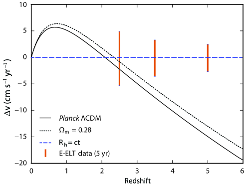
Figure 1: Expected velocity shift $\Delta v$ associated with the redshift drift for the Planck $\Lambda$CDM model ($k=0$, $\Omega_{m}=0.3$ $H_{0}=67.8$ km s^-1 Mpc^-1; solid black), a slight variation with $\Omega_{m}=0.28$, and the $R_{\rm h}=ct$ universe (blue long dash), in which $\Delta v=dz/dt_{0}=0$ at all redshifts. Also shown are the expected $1\sigma$ errors (red) at $z=2.5$, $3.5$, and $5.0$ with the ELT-HIRES after 5 years of monitoring. (Adapted from Martins et al. 2016)

In $R_{\rm h}=ct$, the situation is much simpler. Since $a(t)=t/t_{0}$ in this Universe (see, e.g., Melia 2007, 2016a, 2016b; Melia & Shevchuk 2012), we have

$$H(t)\equiv{\dot{a}\over a}={1\over t}\;.$$ (9)

But from Equation (1), we also see that $(1+z)=t_{0}/t_{e}$. Therefore, $(1+z)=H(t_{e})/H(t_{0})$, or

$$H(t_{e})=H(t_{0})[1+z(t_{0})]\;.$$ (10)

Thus, we conclude from Equation (5) that

$${dz\over dt_{0}}=0\;,$$ (11)

and therefore

$$\Delta v=0$$ (12)

at all redshifts, shown as the blue long-dashed line in figure 1.

According to Liske et al. (2008), the ELT-HIRES is expected to observe the spectroscopic velocity shift with an uncertainty of

$$\sigma_{\Delta v}=1.35{2370\over{\rm S/N}}\sqrt{{30\over N_{\rm QSO}}}\left({5\over 1+z_{\rm QSO}}\right)^{\alpha}\;,$$ (13)

where $\alpha=1.7$ for $z\leq 4$, and $\alpha=0.9$ for $z>4$, with a ${\rm S/N}$ of approximately 1,500 after 5 years of monitoring $N_{\rm QSO}=10$ quasars in each of three redshift bins at $z=2.5$, $3.5$ and $5.0$. These uncertainties (shown in red) are approximately $12$, $8$ and $5$ cm s^-1 yr^-1 at these redshifts. With a baseline of 20 years, the uncertaintes are reduced to approximately $6$, $4$ and $3$ cm s^-1 yr^-1, respectively. Thus, we may already see a $\sim 3\sigma$ difference between the predicted velocity shifts in these two models at $z=5$ after only 5 years. The difference increases to $\sim 5\sigma$ after 20 years.

3 Conclusion

Unlike many other types of cosmological probes, a measurement of the redshift drift of sources moving passively with the Hubble flow offers us the possibility of watching the Universe expand in real time. It does not rely on integrated quantities, such as the luminosity distance, and therefore does not require the pre-assumption of any particular model. Over the next few years, it will be possible to monitor distant sources spectroscopically in order to measure the velocity shift associated with this redshift drift. An accessible goal of this work ought to be a direct one-on-one comparison between the $R_{\rm h}=ct$ Universe and Planck $\Lambda$CDM. The former firmly predicts zero redshift drift at all redshifts, easily distinguishable from all other models associated with a variable expansion rate. Over a 20-year baseline, these measurements will strongly favour one of these models over the other at a $\sim 5\sigma$ confidence level. However, the velocity shifts predicted by these two models at $z\sim 5$ are so different ($-15$ cm s^-1 yr^-1 for the former versus $0$ cm s^-1 yr^-1 for the latter), that even after only 5 years the expected $\sigma_{\Delta v}\sim 5$ cm s^-1 yr^-1 accuracy of the ELT-HIRES may already be sufficient to rule out one of these models relative to the other at a confidence level approaching $3\sigma$.

Should $R_{\rm h}=ct$ emerge as the correct cosmology, the consequences are, of course, quite profound. The reason is that, although certain observational signatures, such as the luminosity distance, can be somewhat similar for these two models at low redshifts (see figure 3 in Melia 2015), they diverge rather quickly in the early universe. So much so that while inflation is required to solve the horizon problem in $\Lambda$CDM, it is not needed (and probably never happend) in $R_{\rm h}=ct$ (Melia 2013b).

References

- (1) Corasaniti, P.-S., Huterer, D. and Melchiorri, A. 2007, PRD, 75, 062001
- (2) Eisenstein, D. J., et al. 2005, ApJ, 633, 560
- (3) Haiman, Z., Mohr, J. J., & Holder, G. P. 2000, ApJ, 553, 545
- (4) Klockner, H.-R., Obreschkow, D., Martins, C.J.A.P., Raccanelli, A., Champion, D., Roy, A. L., Lobanov, A., Wagner, J. and Keller, R. 2015, Proceedings, Advancing Astrophysics with the Square Kilometre Array (AASKA14), PoS AASKA14, 027
- (5) Liske, J. et al. 2008, MNRAS, 386, 1192
- (6) Liske, J. et al. 2014, Top Level Requirements For ELT-HIRES, Document ESO 204697 Version 1
- (7) Loeb, A. 1998, ApJLett, 499, L111
- (8) Martins, C.J.A.P., Martinelli, M., Calabrese, E. and Ramos, M.P.L.P. 2016, arXiv:1606.07261
- (9) Melia, F. 2007, MNRAS, 382, 1917
- (10) Melia, F. 2012, AJ, 144, 110
- (11) Melia, F. 2013a, ApJ, 764, 72
- (12) Melia, F. 2013b, A&A, 553, id. A76
- (13) Melia, F. 2014a, A&A, 561, id. A80
- (14) Melia, F. 2014b, AJ, 147, 120
- (15) Melia, F. 2015, Astroph. Sp. Sci., 356, 393
- (16) Melia, F. 2016a, Frontiers of Physics, 11, 119801
- (17) Melia, F. 2016b, Frontiers of Physics, in press (arXiv:1602.01435)
- (18) Melia, F. & López-Corredoira, M. 2016, Proc. R. Soc. A, submitted [arXiv:1503.05052]
- (19) Melia, F. & McClintock, T. M. 2015, Proc. R. Soc. A, 471, 20150449
- (20) Melia, F. & Shevchuk, A. 2012, MNRAS, 419, 2579
- (21) Percival, W. J., et al. 2007, MNRAS, 381, 1053
- (22) Perlmutter, S., et al. 1999, ApJ, 517, 565
- (23) Pritchard, J. R., Furlanetto, S. R., & Kamionkowski, M. 2007, MNRAS, 374, 159
- (24) Quercellini, C., Amendola, L, Balbi, A., Cabella, P. and Quartin, M. 2012, Phys. Rept., 521, 95
- (25) Refregier, A. 2003, ARAA, 41, 645
- (26) Riess, A. G., et al. 1998, AJ, 116, 1009
- (27) Sandage, A. 1962, ApJ, 136, 319
- (28) Seo, H.-J. & Eisenstein, D. J. 2003, ApJ, 598, 720
- (29) Wei, J.-J., Wu, X., Melia, F. and Maier, R. S. 2015, AJ, 149, 102
- (30) Weinberg, S. 1972, ”Gravitation and Cosmology: Principles and Applications of the General Theory of Relativity” (New York: John Wiley & Sons), 451
- (31) Yu, H.-R., Zhang, T.-J. and Pen, U.-L. 2014, PRL, 113, 041303